1 Feature Selection in Video Classification Yan Liu Computer Science Columbia University Advisor:...

1

Feature Selection in Video Classification

• Yan Liu

• Computer Science

• Columbia University

• Advisor: John R. Kender

Ph.D. Thesis Proposal

2

Outline

• Introduction

• Research progress

• Proposed work

• Conclusion and schedule

1. Introduction

2. Progress

3. Proposal

4. Conclusion

3

1. Introduction

2. Progress

3. Proposal

4. Conclusion

Outline

• Introduction– Motivation of feature selection in video

classification

– Definition of feature selection

– Feature selection algorithm design and evaluation

– Applications of feature selection

• Research progress• Proposed work• Conclusion and schedule

1. Introduction

4

1. Introduction1.1.Motivation1.2.Definition1.3.Components1.4. Applications 2. Progress

3. Proposal

4. Conclusion

Motivation of feature selection in video classification

• The problem of efficient video data management is an important issue – “Semantic gap”: machine learning methods,

such as classification can close it– Efficiency: reducing the dimensionality of the

data prior to processing is necessary

• Feature selection in video classification not well explored– So far, mostly based on researchers’ intuition [A.

Vailaya 2001]

– Goal: select representative features automatically

1.1. Motivation

5

1. Introduction1.1.Motivation1.2.Definition1.3.Components1.4. Applications

2. Progress

3. Proposal

4. Conclusion

Definition of feature selection

• Feature selection focuses on– Finding a feature subset that has the most discriminative

information from the original feature space– Objective: [Guyon 2003]

• Improve the prediction performance• Provide a more cost-effective predictor• Provide a better understanding of the data

• Two major approaches define feature selection [Blum 1997]– Filter methods: emphasize the discovery of relevant

relationships between features and high-level concepts– Wrapper methods: seek a feature subset that minimizes

prediction error of classifying the high-level concept

1.2. Definition

6


3. Proposal

4. Conclusion

Feature selection algorithm design

1.2. Definition

f1, f2, f3, ………………………………….fN

S1{f1}, S2{f2},……..SN{fN}, SN+1{f1, f2} ……………S2N{f1, f2, ……..fN}

Original Feature Space:

Search Algorithm Induction Evaluation

Stop Point

Wrapper Filter

Feature subset Si {f1, f2, ……..fk}, 1 ≦ k N≦

Target Feature Space

7


3. Proposal

4. Conclusion

Three components of feature selection algorithms

1.3. Components

• Search algorithm– Forward selection [Singh 1995]

– Backward elimination [Koller 1996]

– Genetic algorithm [Oliveira 2001]

• Induction algorithm – SVM [Bi 2003], BN [Singh 1995], kNN [Abe 2002], NN

[Oliveira 2001], Boosting [Das 2001]

– Classifier-specific [Weston 2000] and classifier-independent feature selection [Abe 2002]

• Evaluation metric – Distance measure [H. Liu 2002], dependence measure,

consistency measure [Dash 2000], information measure [Koller 1996]

– Predictive accuracy measure (for most wrapper methods)

8

1. Introduction1.1.Motivation1.2.Definition1.3.Components1.4. Applications

2. Progress

3. Proposal

4. Conclusion

Applying feature selection to video classification

1.4. Applications

• Current applications with large data sets– Text categorization [Forman 2003]

– Genetic microarray [Xing 2001]

– Handwritten digit recognition [Oliveira 2001]

– Web classification [Coetzee 2001]

• Applying existing feature selection algorithms to video data– Similar need: massive data, high

dimensionality, complex hypotheses– Difficulty: higher requirement of time cost– Some existing work in video classification

[Jaimes 2000]

9

1. Introduction

2. Progress2.1. BSMT2.2. CSMT2.3. FSMT2.4. Retrieval 3. Proposal

4. Conclusion

Outline

2. Progress

• Introduction • Research progress

– BSMT: Basic Sort-Merge Tree [Liu 2002]

– CSMT: Complement Sort-Merge Tree [Liu 2003]

– FSMT: Fast-converging Sort-Merge Tree [Liu 2004]

– MLFS: Multi-Level Feature Selection [Liu 2003]

– Fast video retrieval system [Liu 2003]

• Proposed work• Conclusion and schedule

10

1. Introduction

2. Progress2.1. BSMT2.1.1. Search2.1.2. Induction2.1.3. Time cost2.1.4. Application2.1.5. Experiment2.2. CSMT2.3. FSMT2.4. Retrieval 3. Proposal

4. Conclusion

Setup Basic Sort-Merge Tree

2.1.1.Search

• Initialize level = 1– N singleton feature subsets

• While level < log2 N

– Induce on every feature subset– Sort subsets based on their classification

accuracy– Combine, pair-wise, feature subsets

11

1. Introduction


4. Conclusion

Search algorithm

2.1.1.Search

A1 (1) A2 A3 A4 A5 A6 A7 A8 A255 A256

B1(2) B2 B3 B4 B128

I1(256)Combine

Sort

Induce

Combine

Sort

Induce

Combine

Sort

Induce

C1(4) C2 C64

Low High

12

1. Introduction


4. Conclusion

Advantages

2.1.1.Search

• To achieve better performance– Avoids local optima of forward selection and

backward elimination

– Avoids heuristic randomness of genetic algorithms

• To achieve lower time cost– Search algorithm is linear in the number of

features – Enables the straightforward creation of near-

optimal feature subsets with little additional work [Liu 2003]

13

1. Introduction


4. Conclusion

Induction algorithm

2.1.2.Induction

• Novel combination of Fastmap and Mahalanobis likelihood

• Fastmap for dimensionality reduction [Faloutsos 1995]

– Feature extraction algorithm approximates PCA with linear time cost

– Reduces the dimensionality of feature subsets to a pre-specified small number

• Mahalanobis maximum likelihood for classification [Duda 2000]

– Computes the likelihood that a point belongs to a distribution that is modeled as a multidimensional Gaussian with arbitrary covariance

– Works well for video domain

14

1. Introduction


4. Conclusion

Applications to instructional video frame categorization

2.1.4. Application

• Pre-processing:– Temporally subsample: every other I frame (one

frame/sec)

– Spatially subsample: six DC terms of each macro-block

• Feature selection– From 300 six-dimensional features to r features

• Video segmentation and retrieval– Classify frames or segments in the usual way

using the resulting feature subset

15

1. Introduction


4. Conclusion

Test bed of instructional video frame categorization

2.1.5. Experiment

• Classify instructional video of a 75 minute lecture in MPEG-1 format– 4700 video frames with 300 six-dimensional features– 400 training data for feature selection and classification

training– Classify to four categories

• Benchmarks: Random feature selection for 100 times– Experiments differ only in selected features– Any other benchmark is intractable on video dataset

Handwriting Announcement Demo Discussion

16

1. Introduction


4. Conclusion

Accuracy improvement

2.1.5. Experiment

0

0.01

0.02

0.03

0.04

0.05

0.06

1 2 3 4 5 6 7 8 9 10

Fastmap dimensions c from 1 to 10

Err

or

rate

Mean of Random Sort-Merge

Comparison of frame categorization error rate using 30 (of 300) features selected by BSMT: nearly perfect!

17

1. Introduction


4. Conclusion

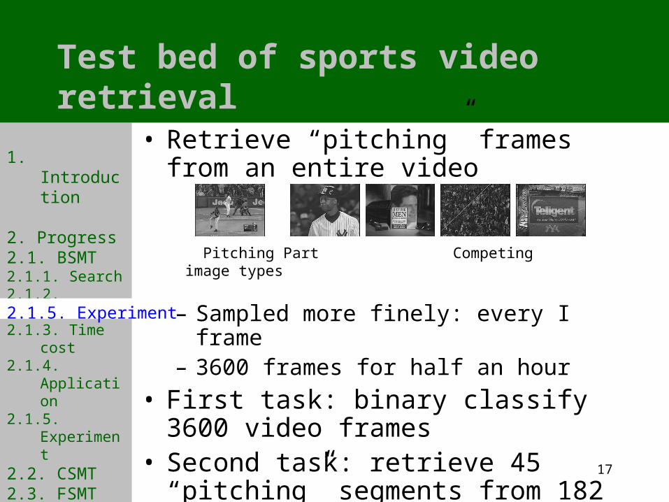
Test bed of sports video retrieval

2.1.5. Experiment

Pitching Part Competing image types

• Retrieve “pitching” frames from an entire video

– Sampled more finely: every I frame – 3600 frames for half an hour

• First task: binary classify 3600 video frames• Second task: retrieve 45 “pitching” segments

from 182 pre-segmented video segments

18

1. Introduction


4. Conclusion


2.1.5. Experiment

Fixed Fastmap dimension: c = 2 Different sample rate r: from 2 to 32

Precision: percentage of items classified as positive that actually are positive (left bars in graphs)Recall: percentage of positives that are classified as positives (right bars in graphs)

r = 2 r = 8 r = 16 r = 32

Feature number r = 8

0

0.1

0.2

0.3

0.4

0.5

0.6

0.7

0.8

0.9

1

Precision Recall



0

0.1

0.2

0.3

0.4

0.5

0.6

0.7

0.8

0.9

1

Precision Recall



0

0.1

0.2

0.3

0.4

0.5

0.6

0.7

0.8

0.9

1

Precision Recall



0

0.1

0.2

0.3

0.4

0.5

0.6

0.7

0.8

0.9

1

Precision Recall


19

1. Introduction

2. Progress2.1. BSMT2.2. CSMT2.2.1. Sparse train2.2.2. Search2.2.3. Experiment2.3. FSMT2.4. Retrieval 3. Proposal

4. Conclusion

Adapting to sparse training data

2.2.1. Sparse train

• Difficulties of feature selection in video, as in genetic microarray data– Huge feature sets with 7130 dimensions – Small training data sets with 38 training data

• Renders some feature selection algorithm ineffective [Liu 2003]– More coarsely quantized prediction error– Randomness accumulates with the choice of each feature,

influencing the choice of its successors • Existing feature selection for microarray data is a model for

video [Xing 2001]– Forward search based on information gain: 7130 features

reduced to 360– Backward elimination based on Markov Blanket: 360 features

reduced to 100 or less– Leave-one-out cross-validation decides the best size of the

feature subset

20

1. Introduction


4. Conclusion

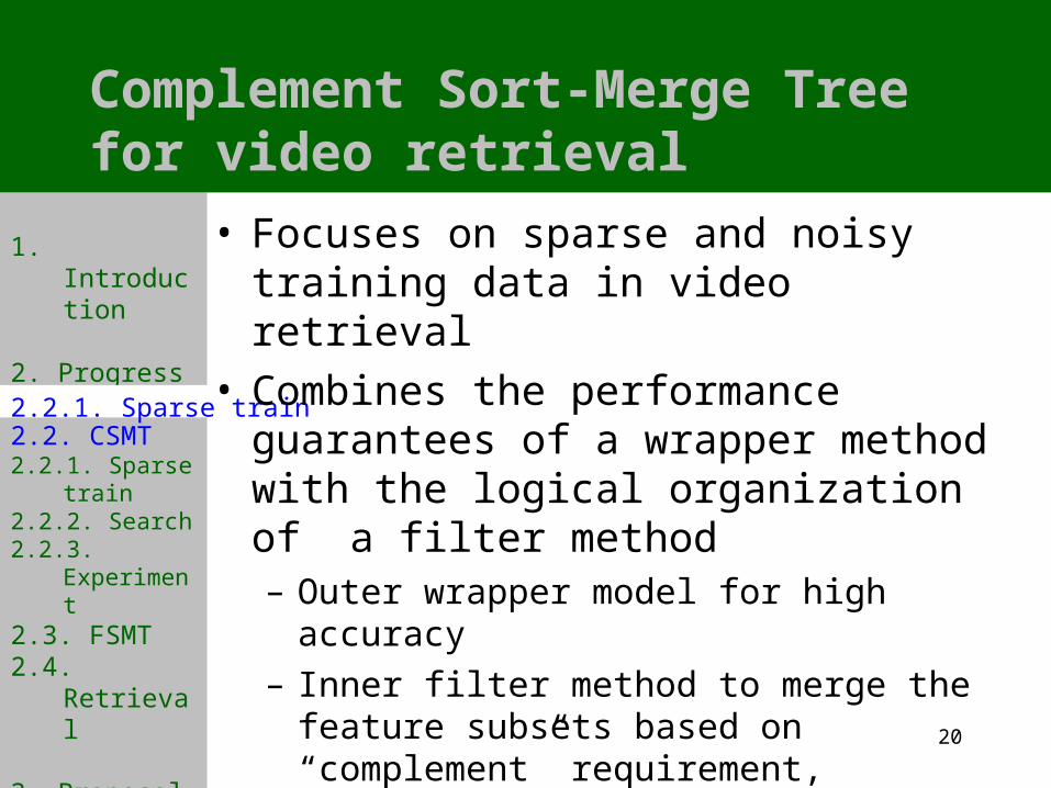
Complement Sort-Merge Tree for video retrieval

2.2.1. Sparse train

• Focuses on sparse and noisy training data in video retrieval

• Combines the performance guarantees of a wrapper method with the logical organization of a filter method– Outer wrapper model for high accuracy

– Inner filter method to merge the feature subsets based on “complement” requirement, addressing the limitation of sparse training data

21

1. Introduction


4. Conclusion

Search algorithm

2.2.2. Search

Illustration of CSMT for N = 256.

Complement

Sort

Induce

Complement

Sort

Induce

Complement

Sort

Induce

A1 A2 A5 A6 A255 A256

C1 C2 C64

B1 B2 B3 B4 B128

I1

• Leaves: singleton feature subsets;

• White nodes: unsorted feature subsets

• Gray nodes: white nodes rank-ordered by performance.

• Black nodes: pairwise mergers of gray nodes, with pairs formed under the complement requirement.

22

1. Introduction


4. Conclusion

Complement test

2.2.2. Search

Illustration of complement test of CSMT for the A level of last slide

• Suppose the sorted singletons A1’ and A3’are paired to form pair B1

• To finding a paring for A2’, examine A4,’ A5’, A6’, which have the same error rate on the m training samples

• The bitwise OR of performance vectors of A2’ and A5’ maximizes the performance coverage

• Therefore, A5’ complements A2’ for B2

Sort

Induce

Complement

0

0

0

.

.

.

1

1

1

1

0

0

1

.

.

.

0

1

1

1

0

1

1

.

.

.

0

0

1

1

0

0

0

.

.

.

1

1

1

1

0

0

0

.

.

.

0

1

1

1

A1 A2 A3 A4 A5 A6 A7

B1 B2 B3

A1’ A2’ A3’ A4’ A5’ A6’ A7’

A1’’ A2’’ A3’’ A4’’ A5’’ A6’’ A7’‘

23

1. Introduction


4. Conclusion

Test bed for video retrieval

2.2.3. Experiment

• Retrieve “announcements” frames from an entire video with 4500 frames

• No prior temporal segmentation or other pre-processing.

•

• Only 80 training data, including considerable noise:

Announcement Competing image types

Clean training data But also, noisy training data

24

1. Introduction


4. Conclusion


2.2.3. Experiment

• Fixed sample rate: r = 8

• Different dimension c: from 1 to 10

• Same dimension c = 4

• Different sample rate r: from 2 to 16

0

0.005

0.01

0.015

0.02

0.025

0.03

0.035

0.04

0.045

1 2 3 4 5 6 7 8 9 10

Fastmap dimension c (1~10)

Err

or

rate

Mean of Random CSMT

0

0.002

0.004

0.006

0.008

0.01

0.012

0.014

0.016

0.018

2 4 8 16

Number of featuresE

rro

r ra

te

Mean of Random CSMT

25

1. Introduction


4. Conclusion

Test bed of shot classification

2.2.3. Experiment

• Retrieve “emphasis” frames in an instructional video of MPEG-1 format– More subtle, semantically-defined class– Segment into 69 shots

• 3600 test data ( i.e. every I frame of a 60 minute video)

• 200 training data, from 10 example sequences

Emphasis part Non-emphasis part

26

1. Introduction


4. Conclusion


2.2.3. Experiment

Error rate of CSMT vs. random for retrieval of “emphasis” with features r fixed at 16.

27

1. Introduction

2. Progress2.1. BSMT2.2. CSMT2.3. FSMT2.3.1. Search2.3.2. Experiment2.4. Retrieval 3. Proposal

4. Conclusion

Fast-converging Sort-Merge Tree

2.3. FSMT

• Focuses on the problem of – Over-learning data sets– On-line retrieval requirement

• Sets up selected parts of the feature selection tree to save time, without sacrificing accuracy

• Uses information gain as an evaluation metric, instead of prediction error in BSMT

• Controls the convergence speed (amount of pruning at each level ) based on user’s requirement

28

1. Introduction


4. Conclusion

Search algorithm

2.3.1. Search

• Initialize level = 0– N singleton feature subsets.– Calculate R: number of features retained at

each level, based desired convergence rate and the goal of r features at conclusion.

• While level < log2 r +1 – Induce on every feature subset.– Sort subsets based on information gain.– Prune the level based on R.– Combine, pair-wise, feature subsets form

those remaining.

29

1. Introduction


4. Conclusion

FSMT of constant converge rate

2.3.1. Search

E1 E2

D1 D2 D8

C1 C2 C32

B1 B2 B128

A1 A2 A512

F1 F2 F1800

v0=1

r1 = 16v1 = 2r2 = 8v2 = 8r3 = 4v3 = 32r4 = 2v4 = 128r5 = 1v5 = 512

30

1. Introduction


4. Conclusion


2.3.2. Experiment

• Same test bed with BSMT

• 1800 single-dimensional features

• Better performance than random feature selection and similar performance with CSMT ( r = 16 )

• The number of inductions is only 682 using FSMT, compared with 4095 using BSMT or CSMT

0

0.005

0.01

0.015

0.02

0.025

0.03

0.035

1 2 3 4 5 6 7 8 9 10

Fastmap dimension c (1~10)

Mean of Random FSMT1 FSMT2

31

1. Introduction


4. Conclusion

Stable performance

2.3.2. Experiment

Although FSMT is an application-driven algorithm, it does retain some of the advantages of BSMT.

0

0. 005

0. 01

0. 015

2 4 8 16

Number of f eat ur es

Mean of Random FSMT

• Fixed sample rate: r = 8

• Different dimension c: from 1 to 10.

• Same dimension: c = 4

• Different sample rate r: from 2 to 16.

32

1. Introduction

2. Progress2.1. BSMT2.2. CSMT2.3. FSMT2.4. Retrieval2.4.1. MLFS2.4.2. Lazy Eval. 2.4.3. Experiment 3. Proposal

4. Conclusion

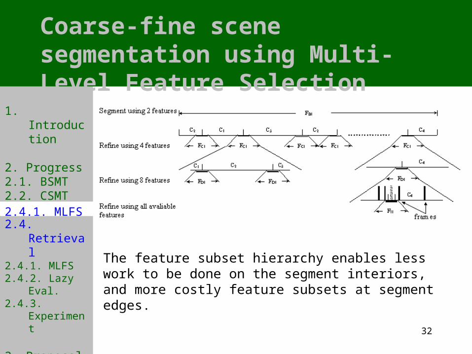
Coarse-fine scene segmentation using Multi-Level Feature Selection

2.4.1. MLFS

The feature subset hierarchy enables less work to be done on the segment interiors, and more costly feature subsets at segment edges.

33

1. Introduction


4. Conclusion

How to define the parameters

2.4.1. MLFS

• Ri: Feature subset size (2, 4, 8 , . . .)

– Increases with i and therefore increases the classification accuracy

• Li: Neighborhood parameter (uncertainty region in

video)

– Remains constant or decreases with i and therefore focuses the attention of the more costly classifier

• Si: Decision threshold (of certainty of segmentation)

– Si = Pr(Cj) - Pr(Ck) k = 1, 2 … n and k j

– Pr(Cj) is the maximum Mahalanobis likelihood among

all categories using this feature subset

– Ensures that classification is correct and unambiguous

34

1. Introduction


4. Conclusion

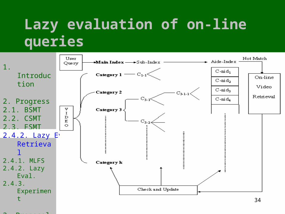
Lazy evaluation of on-line queries

2.4.2. Lazy Eval.

35

1. Introduction


4. Conclusion

Efficiency improvement

2.4.3. Experiment

• Using same test bed of BSMT

• Only 3.6 features are used per frame

• With similar performance of 30 features selected by BSMT

36

1. Introduction

2. Progress2.1. BSMT2.2. CSMT2.3. FSMT2.4. Retrieval

3. Proposal

4. Conclusion

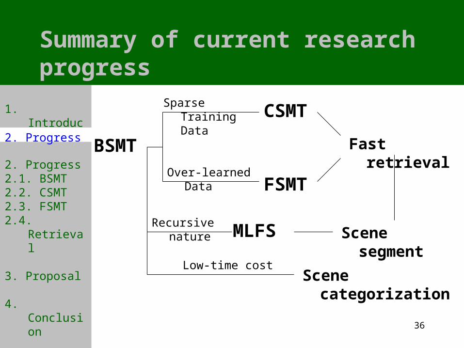
Summary of current research progress

2. Progress

BSMT

CSMT

FSMT

MLFS

Sparse Training Data

Over-learned Data

Fast retrieval

Scene segment

Scene categorization

Recursive nature

Low-time cost

37

1. Introduction

2. Progress

3. Proposal

4. Conclusion

Outline

3. Proposal

• Introduction• Research progress• Proposed work

• Improve current feature selection algorithm

• Algorithm evaluation

• New Applications

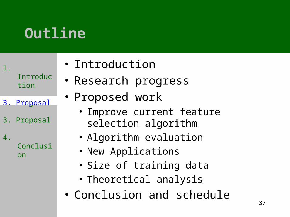
• Size of training data

• Theoretical analysis

• Conclusion and schedule

38

1. Introduction

2. Progress

3. Proposal3.1. Improve3.2. Evaluation3.3. Application3.4. Train size3.5. Theory

4. Conclusion

Improvements to current algorithms

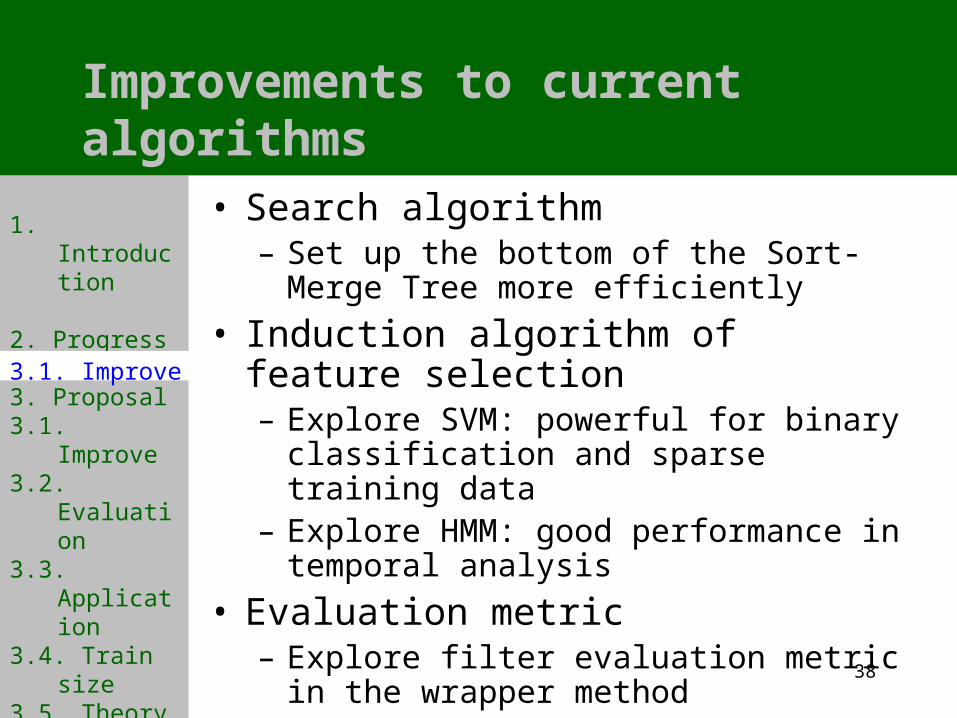
3.1. Improve

• Search algorithm– Set up the bottom of the Sort-Merge Tree more

efficiently

• Induction algorithm of feature selection– Explore SVM: powerful for binary

classification and sparse training data– Explore HMM: good performance in temporal

analysis

• Evaluation metric– Explore filter evaluation metric in the wrapper

method

39

1. Introduction

2. Progress


4. Conclusion

Algorithm evaluation

3.2. Evaluation

• Accuracy– Classification evaluation: Error rate, Balanced Error

Rate (BER), Received Operating Characteristic (ROC) Curve, Area Under Curve (AUC)

– Video analysis evaluation: Precision, Recall, F-measure

• Efficiency – Selected feature subsets size: Fraction of Features (FF),

best size of feature subset– Time cost: of search algorithm, of induction algorithm;

stopping point

• Dependence– How to choose proper classifier– How to compare feature selection algorithms in certain

applications

40

1. Introduction

2. Progress


4. Conclusion

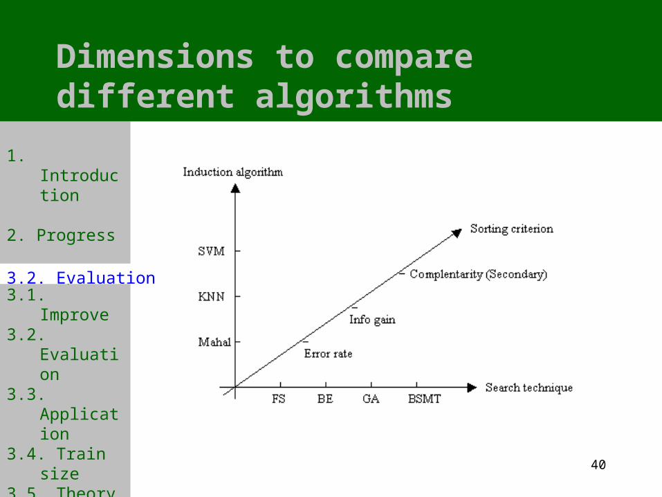
Dimensions to compare different algorithms

3.2. Evaluation

41

1. Introduction

2. Progress


4. Conclusion

New applications

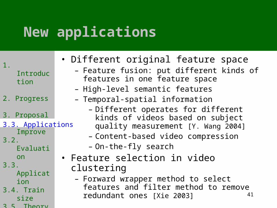
3.3. Applications

• Different original feature space– Feature fusion: put different kinds of features in one

feature space– High-level semantic features – Temporal-spatial information

– Different operates for different kinds of videos based on subject quality measurement [Y. Wang 2004]

– Content-based video compression– On-the-fly search

• Feature selection in video clustering – Forward wrapper method to select features and filter

method to remove redundant ones [Xie 2003]

42

1. Introduction

2. Progress


4. Conclusion

Extension to training data set extremes

3.4. Train size

• Sparse training data– Better feature selection algorithms – Use training data efficiently in cross-validation

• Massive training data– Random selection based on two assumptions: feature subset performance

stability, and training set independence– Methods to extract a representative training data subset for feature selection

• Non-balanced training data– Positive examples are sparse, negative examples are massive and must be

sampled – Video retrieval in large database is non-balanced

• One class training data– Feature selection for one class training in masquerade (computer security

violation) detection [K. Wang 2003]– Select features using one class training in video retrieval

43

1. Introduction

2. Progress

3. Proposal

4. Conclusion

Outline

4. Conclusion

• Introduction

• Research progress

• Proposed work

• Conclusion and schedule– Finished work and further work– Schedule

44

Finished work and further work

Feature Selection Applications

Search Algorithm

CSMT

BSMT

MLFS

FSMT

Induction Algorithm

Evaluation Metric

Algorithm Evaluation

Challenge

discussionStop point

Over-fitting

Training dataset

Retrieval

Video

Classification

Categorization

Segmentation

Clustering

CompressionOther

applications

New feature setOn-the-fly

search

Theoretical Analysis

Gene microarray

Audio

Mostly done

Partly done

Mostlyundone

Half done

45

1. Introduction

2. Progress

3. Proposal

4. Conclusion4.1. Conclusion4.2. Schedule

Task Schedule

4.2. Schedule

46

1. Introduction

2. Progress

3. Proposal

4. Conclusion

Ph.D. Thesis Proposal

Thank you!

1 Feature Selection in Video Classification Yan Liu Computer Science Columbia University Advisor:...

Documents

Transcript of 1 Feature Selection in Video Classification Yan Liu Computer Science Columbia University Advisor:...