1 Faculty of Social Sciences Induction Block: Maths & Statistics Lecture 1 Overview; Variables,...
41
1 Faculty of Social Sciences Induction Block: Maths & Statistics Lecture 1 Overview; Variables, Constants, Tables & Graphs Dr Gwilym Pryce
-
Upload
caroline-perry -
Category
Documents
-
view
214 -
download
0
Transcript of 1 Faculty of Social Sciences Induction Block: Maths & Statistics Lecture 1 Overview; Variables,...
1
Faculty of Social Sciences Induction Block: Maths & Statistics Lecture 1
Overview; Variables, Constants, Tables & Graphs
Dr Gwilym Pryce
2
Aims and Objectives of the Maths & Stats Induction
Aim: to revise basic maths relevant to the course.
Objectives: by the end of the Induction Programme students should be able to:
• Understand the meaning and types of variables and constants
• Understand how to graph scale and categorical variables• Be familiar with basic algebraic notation• Understand the simple mathematical representation of
relationships, both algebraically and graphically• Understand the basic principles and laws of probability• Outline the main issues surrounding sampling.
3
Why do social scientists need to learn about statistics? Theories have to be verified empirically otherwise
they remain conjectures Need for evidenced based practice & policy:
– medicine
– public health
– economics informed decisions better than uninformed
decisions information is complex and needs summarising in a
way that reflects the underlying data in a meaningful way
4
Why do we need mathematics?
Statistics can be represented in a non-mathematical way, but some understanding and application of maths will help us:– spoken language can be ambiguous varies
across countries and cultures
5
Different cultures find different things funny Different cultures and languages express ideas
differently But mathematical notation is:
– unambiguous and concise– common notation is understood across cultures
and languages Research & ideas expressed mathematically
can easily reach an international audience
6
Plan of Maths & Stats Induction Lecture 1: Variables, Constants, Tables &
Graphs Lecture 2: Algebra and Notation Lecture 3: Precise and Approx Relationships
between variables Lecture 4: Probability Lecture 5: Inference Lecture 6: Hypothesis tests Tutorial: Samples and populations; Validity
and Reliability
7
Plan of Maths & Stats Lecture 1: Variables and Constants 1. What is a variable? 2. What is a constant? 3. Types of variables 4. Graphs of single variables
– Why summarise?– Tables & graphs of categorical data– Tables & Graphs of Continuous /
Quantitative/Scale variables
8
1. What is a variable?– A measurement or quantity that can take on
more than one value:• E.g. size of planet: varies from planet to planet• E.g. weight: varies from person to person• E.g. gender: varies from person to person• E.g. fear of crime: varies from person to person• E.g. income: varies from HH to HH
– I.e. values vary across ‘individuals’ = the objects described by our data
9
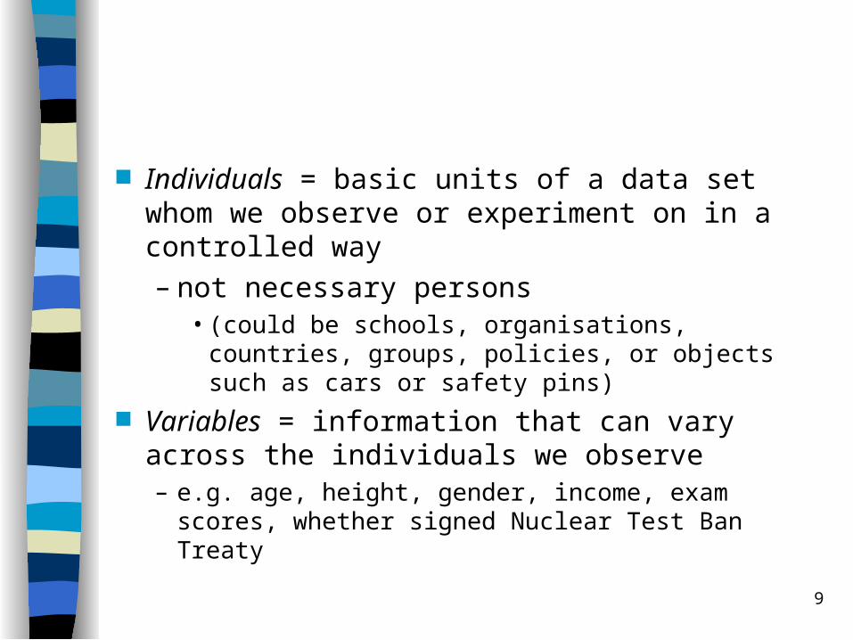
Individuals = basic units of a data set whom we observe or experiment on in a controlled way– not necessary persons
• (could be schools, organisations, countries, groups, policies, or objects such as cars or safety pins)
Variables = information that can vary across the individuals we observe– e.g. age, height, gender, income, exam scores,
whether signed Nuclear Test Ban Treaty
10
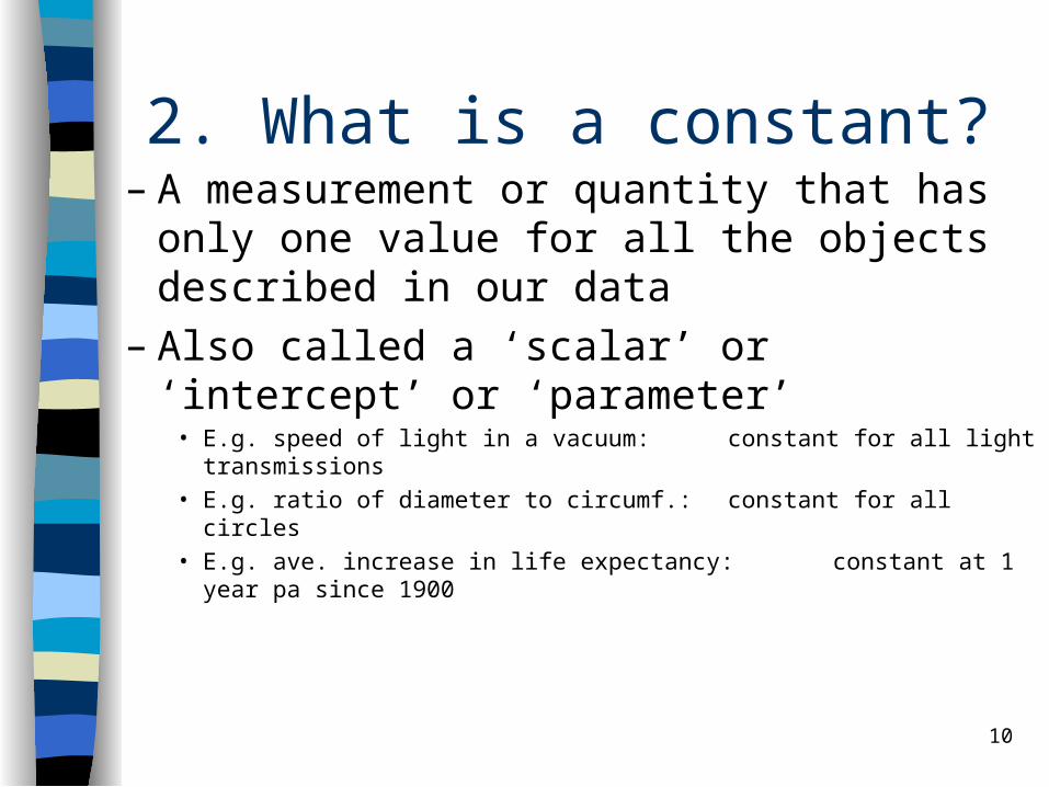
2. What is a constant?– A measurement or quantity that has only one
value for all the objects described in our data– Also called a ‘scalar’ or ‘intercept’ or ‘parameter’
• E.g. speed of light in a vacuum: constant for all light transmissions• E.g. ratio of diameter to circumf.: constant for all circles• E.g. ave. increase in life expectancy: constant at 1 year pa since 1900
11
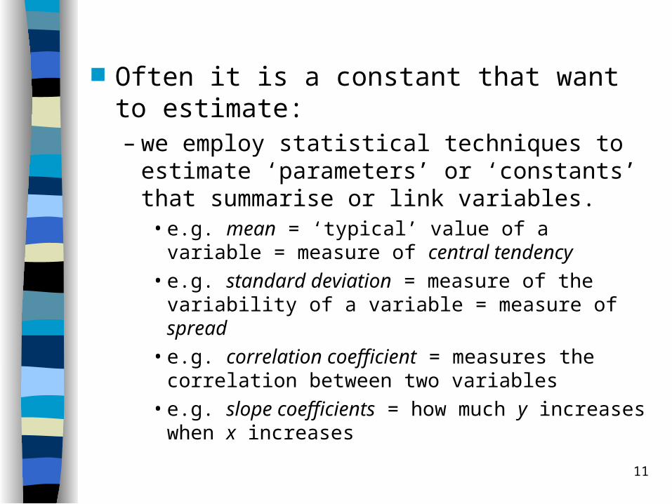
Often it is a constant that want to estimate:– we employ statistical techniques to estimate
‘parameters’ or ‘constants’ that summarise or link variables.
• e.g. mean = ‘typical’ value of a variable = measure of central tendency
• e.g. standard deviation = measure of the variability of a variable = measure of spread
• e.g. correlation coefficient = measures the correlation between two variables
• e.g. slope coefficients = how much y increases when x increases
12
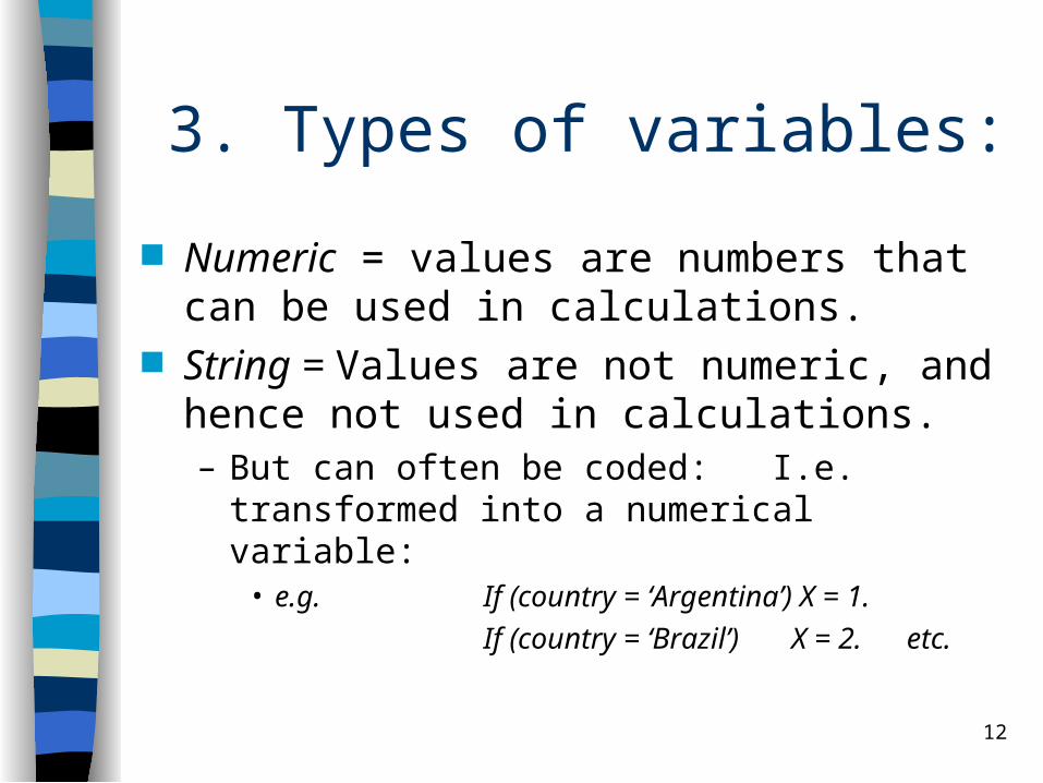
3. Types of variables:
Numeric = values are numbers that can be used in calculations.
String = Values are not numeric, and hence not used in calculations. – But can often be coded: I.e. transformed into a
numerical variable:• e.g. If (country = ‘Argentina’) X = 1.
If (country = ‘Brazil’) X = 2. etc.
13
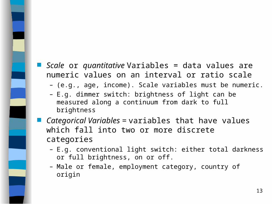
Scale or quantitative Variables = data values are numeric values on an interval or ratio scale – (e.g., age, income). Scale variables must be numeric.– E.g. dimmer switch: brightness of light can be measured
along a continuum from dark to full brightness
Categorical Variables = variables that have values which fall into two or more discrete categories – E.g. conventional light switch: either total darkness or full
brightness, on or off.– Male or female, employment category, country of origin
14
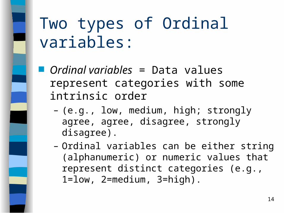
Two types of Ordinal variables:
Ordinal variables = Data values represent categories with some intrinsic order – (e.g., low, medium, high; strongly agree, agree,
disagree, strongly disagree). – Ordinal variables can be either string
(alphanumeric) or numeric values that represent distinct categories (e.g., 1=low, 2=medium, 3=high).
15
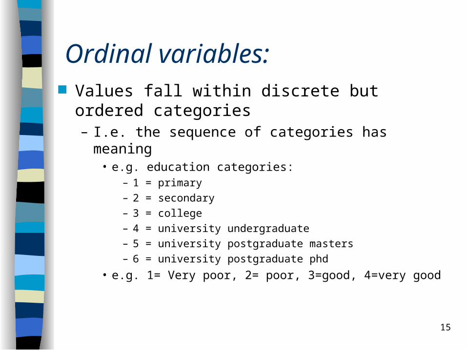
Ordinal variables: Values fall within discrete but ordered
categories– I.e. the sequence of categories has meaning
• e.g. education categories:– 1 = primary
– 2 = secondary
– 3 = college
– 4 = university undergraduate
– 5 = university postgraduate masters
– 6 = university postgraduate phd
• e.g. 1= Very poor, 2= poor, 3=good, 4=very good
16
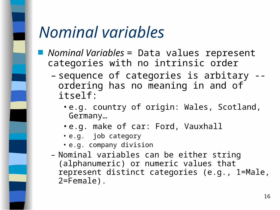
Nominal variables Nominal Variables = Data values represent
categories with no intrinsic order – sequence of categories is arbitary --
ordering has no meaning in and of itself:• e.g. country of origin: Wales, Scotland,
Germany…• e.g. make of car: Ford, Vauxhall• e.g. job category • e.g. company division
– Nominal variables can be either string (alphanumeric) or numeric values that represent distinct categories (e.g., 1=Male, 2=Female).
17
4. Graphs of Variables:
Why summarise? Tables & graphs of categorical data Tables & Graphs of Continuous /
Quantitative/Scale variables
18
Why Summarise? Small data sets can be presented in their
entirety• e.g. if only have 10 observations and 3 variables, can
list all data• but even then we might want to know what is the
typical value of a variable
Large data sets require summary Lots of information can be confusing,
particularly if numerical• most of us need headline figures or stylised facts to be
able to absorb information.
19
Graphical summaries:– allow us to visualise the distribution of data
across different values or categories• how many (or what proportion) of cases fall
within certain categories or ranges of values?
Summary statistics:– describe the distribution of a single variable
20
Categories are listed either in columns or rows (respecting order if ordinal)
• Count or % of cases in each category listed
If number of categories is large, may be useful to group categories together:
• e.g. Country of origin ---> collapse to continents Good tables:
• give clear messages: tell a story• too much info in a table defeats its purpose• Source always given
Tables of Categorical Data

21
Income Support claimants with housing costs by statistical group:May 1999
Total(All
Claimantswith
MortgageInterest)
Aged 60 orover
LoneParents
Disabled Other
000s 000s % 000s % 000s % 000s %1999 263 93 35 67 25 88 33 15 6
DSS Quarterly Statistical Enquiry

22
Income Support claimants with housing costs by statistical group:May 1993 to May 1999
Total(All
Claimantswith
MortgageInterest)
Aged 60 orover
LoneParents
Disabled Other
000s 000s % 000s % 000s % 000s %1993 284 88 31 107 38 63 22 27 101994 310 96 31 115 37 74 24 25 81995 329 102 31 115 35 87 26 25 81996 322 103 32 104 32 89 28 25 81997 301 98 33 92 31 89 30 22 71998 281 96 34 78 28 90 32 17 61999 263 93 35 67 25 88 33 15 6
DSS Quarterly Statistical Enquiry
23
Graphs of Categorical Data
Pie Charts– If all the categories sum to a meaningful
total, then you can use a pie chart– Pie charts emphasise the differences in
proportions between categories– OK for a single snapshot, but not very
good for showing trends• would need to have a separate pie chart for
each year
24
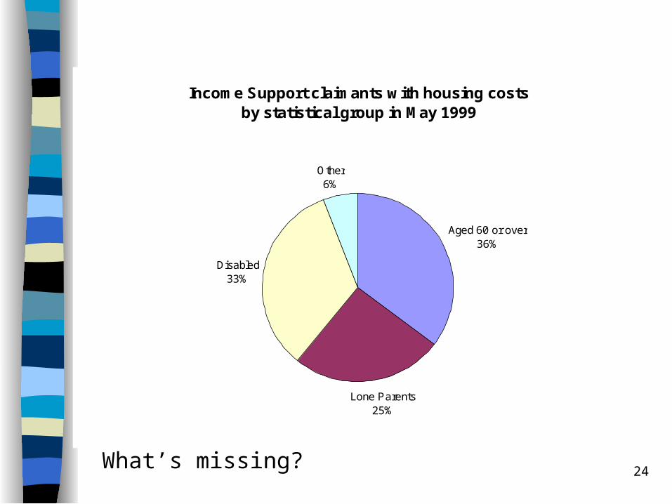
Income Support claimants with housing costs by statistical group in May 1999
Aged 60 or over36%
Lone Parents25%
Disabled33%
Other6%
What’s missing?
25
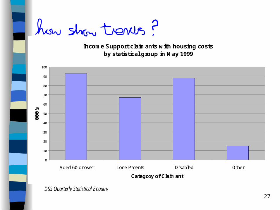
Bar Charts– can show either % or count– not very good for showing trends in more
than one category
26
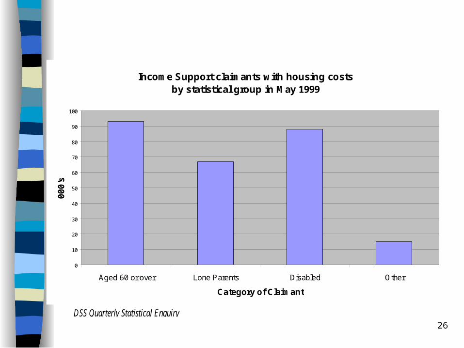
Income Support claimants with housing costs by statistical group in May 1999
0
10
20
30
40
50
60
70
80
90
100
Aged 60 or over Lone Parents Disabled Other
Category of Claimant
00
0's
DSS Quarterly Statistical Enquiry
27
Income Support claimants with housing costs by statistical group in May 1999
0
10
20
30
40
50
60
70
80
90
100
Aged 60 or over Lone Parents Disabled Other
Category of Claimant
00
0's
DSS Quarterly Statistical Enquiry

28
1993 19941995
19961997
19981999
Other 000s
Disabled 000s
Lone Parents 000s
Aged 60 or over 000s0
20
40
60
80
100
120
000's
Year
Category
Income Support claimants with housing costs by statistical group: May 1993 to May 1999
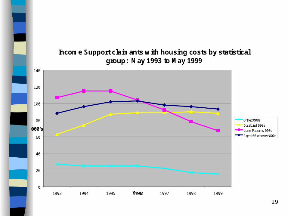
DSS Quarterly Statistical Enquiry
29
Income Support claimants with housing costs by statistical group: May 1993 to May 1999
0
20
40
60
80
100
120
140
1993 1994 1995 1996 1997 1998 1999Year
000's
Other 000s
Disabled 000s
Lone Parents 000s
Aged 60 or over 000s

30
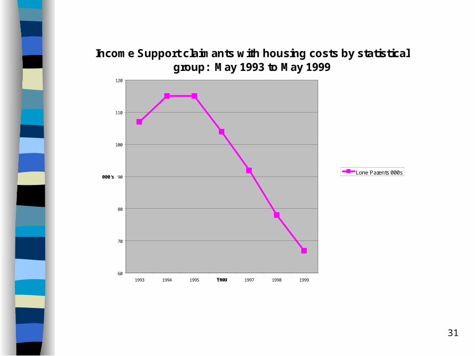
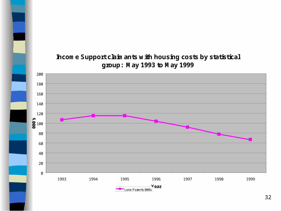
Beware of scaling...
31
Income Support claimants with housing costs by statistical group: May 1993 to May 1999
60
70
80
90
100
110
120
1993 1994 1995 1996 1997 1998 1999Year
000'sLone Parents 000s
32
Income Support claimants with housing costs by statistical group: May 1993 to May 1999
0
20
40
60
80
100
120
140
160
180
200
1993 1994 1995 1996 1997 1998 1999
Year
000'
s
Lone Parents 000s
33
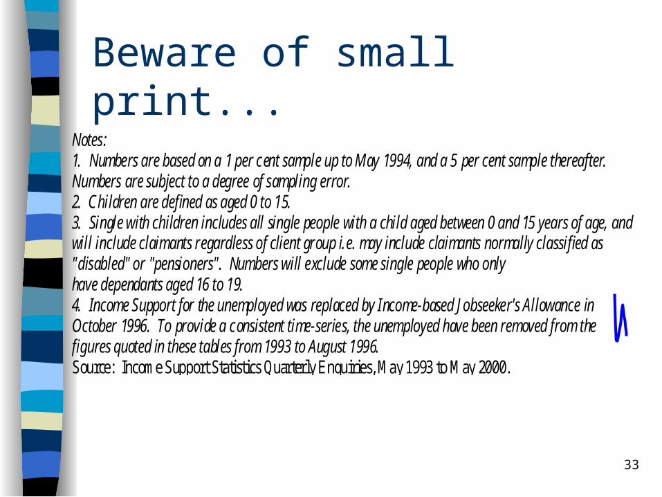
Beware of small print...Notes:1. Numbers are based on a 1 per cent sample up to May 1994, and a 5 per cent sample thereafter.Numbers are subject to a degree of sampling error.2. Children are defined as aged 0 to 15.3. Single with children includes all single people with a child aged between 0 and 15 years of age, andwill include claimants regardless of client group i.e. may include claimants normally classified as"disabled" or "pensioners". Numbers will exclude some single people who onlyhave dependants aged 16 to 19.4. Income Support for the unemployed was replaced by Income-based Jobseeker's Allowance inOctober 1996. To provide a consistent time-series, the unemployed have been removed from thefigures quoted in these tables from 1993 to August 1996.Source: Income Support Statistics Quarterly Enquiries, May 1993 to May 2000.
34
Tabulating and Graphing Scale Data Scale or quantitative data: usually a
measurement of size or quantity– not meaningful to report % or count unless
break into categories (& then it becomes categorical data!)
• e.g. income
Tables of raw data not much use unless only a few values...
35
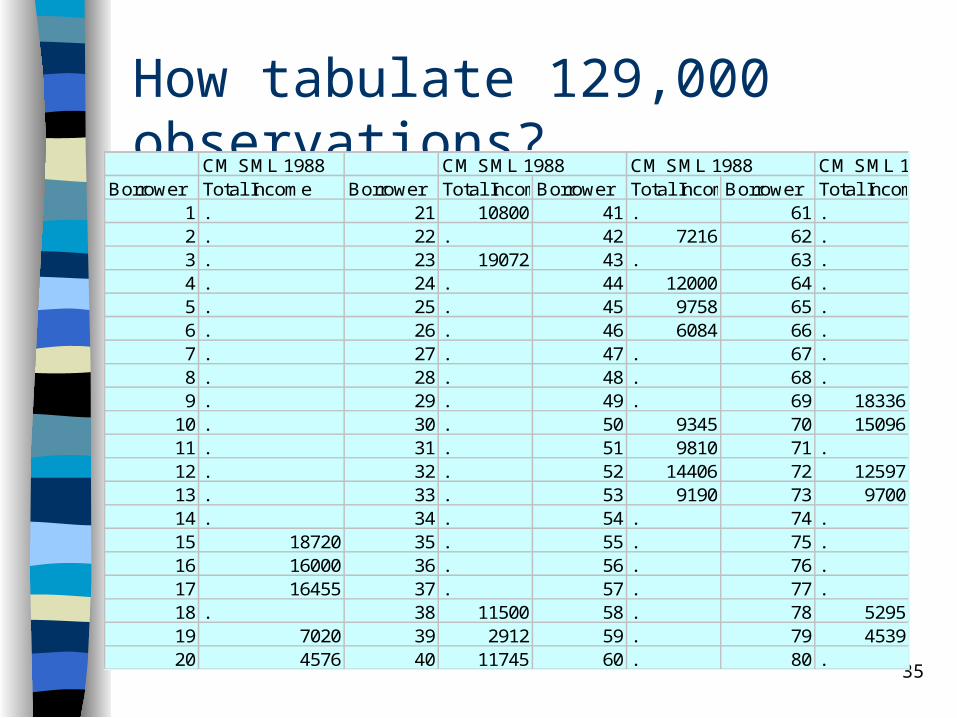
How tabulate 129,000 observations?CM SML 1988 CM SML 1988 CM SML 1988 CM SML 1988
Borrower Total Income Borrower Total IncomeBorrower Total IncomeBorrower Total Income1 . 21 10800 41 . 61 .2 . 22 . 42 7216 62 .3 . 23 19072 43 . 63 .4 . 24 . 44 12000 64 .5 . 25 . 45 9758 65 .6 . 26 . 46 6084 66 .7 . 27 . 47 . 67 .8 . 28 . 48 . 68 .9 . 29 . 49 . 69 18336
10 . 30 . 50 9345 70 1509611 . 31 . 51 9810 71 .12 . 32 . 52 14406 72 1259713 . 33 . 53 9190 73 970014 . 34 . 54 . 74 .15 18720 35 . 55 . 75 .16 16000 36 . 56 . 76 .17 16455 37 . 57 . 77 .18 . 38 11500 58 . 78 529519 7020 39 2912 59 . 79 453920 4576 40 11745 60 . 80 .
36
What are we interested in when describing the income data?– Is income evenly spread?– Or are most people rich?– Or are most people poor?– Or are most reasonably well off?
This are all questions about the variable’s Distribution– We can represent the whole data set with
one picture...
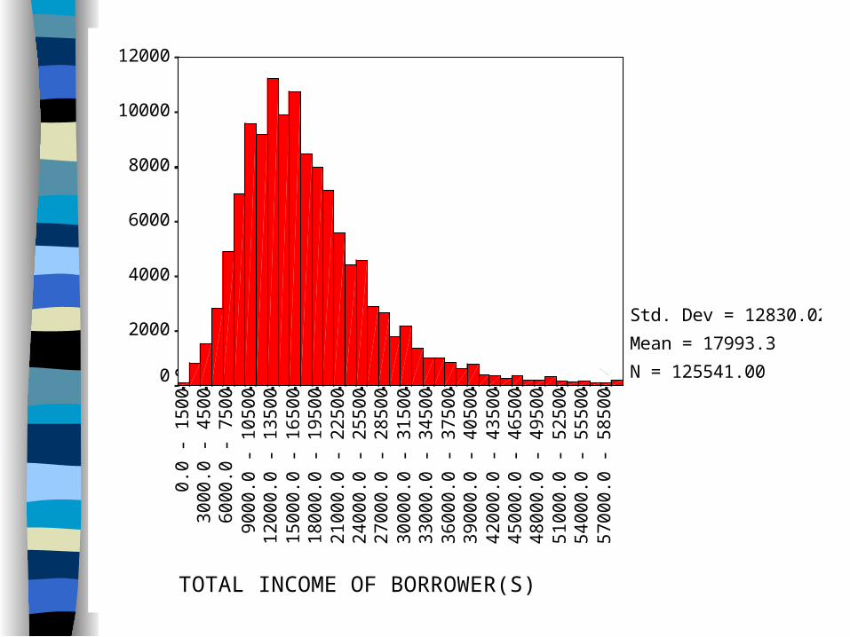
37TOTAL INCOME OF BORROWER(S)5
70
00
.0 -
58
50
0.0
54
00
0.0
- 5
55
00
.05
10
00
.0 -
52
50
0.0
48
00
0.0
- 4
95
00
.04
50
00
.0 -
46
50
0.0
42
00
0.0
- 4
35
00
.03
90
00
.0 -
40
50
0.0
36
00
0.0
- 3
75
00
.03
30
00
.0 -
34
50
0.0
30
00
0.0
- 3
15
00
.02
70
00
.0 -
28
50
0.0
24
00
0.0
- 2
55
00
.02
10
00
.0 -
22
50
0.0
18
00
0.0
- 1
95
00
.01
50
00
.0 -
16
50
0.0
12
00
0.0
- 1
35
00
.09
00
0.0
- 1
05
00
.06
00
0.0
- 7
50
0.0
30
00
.0 -
45
00
.00
.0 -
15
00
.0
12000
10000
8000
6000
4000
2000
0
Std. Dev = 12830.02
Mean = 17993.3
N = 125541.00
38LTV16
.75
- 17
.25
15.7
5 -
16.2
514
.75
- 15
.25
13.7
5 -
14.2
512
.75
- 13
.25
11.7
5 -
12.2
510
.75
- 11
.25
9.75
- 1
0.25
8.75
- 9
.25
7.75
- 8
.25
6.75
- 7
.25
5.75
- 6
.25
4.75
- 5
.25
3.75
- 4
.25
2.75
- 3
.25
1.75
- 2
.25
.75
- 1.
25-.
25 -
.25
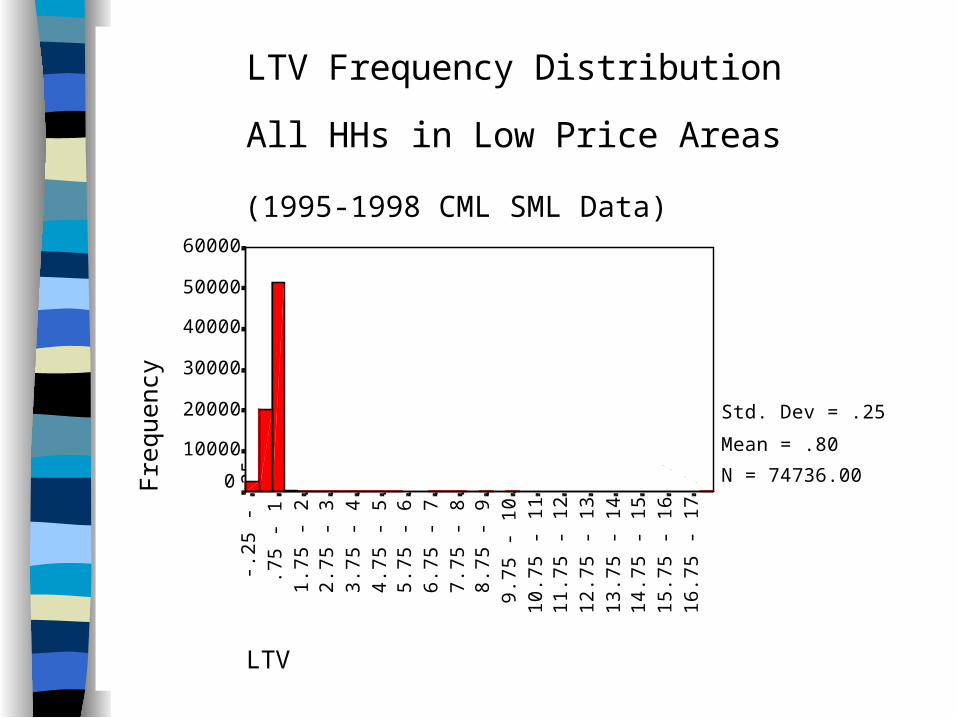
LTV Frequency Distribution
All HHs in Low Price Areas
(1995-1998 CML SML Data)
Fre
quen
cy
60000
50000
40000
30000
20000
10000
0
Std. Dev = .25
Mean = .80
N = 74736.00
39LTV
1.45
- 1
.50
1.40
- 1
.45
1.35
- 1
.40
1.30
- 1
.35
1.25
- 1
.30
1.20
- 1
.25
1.15
- 1
.20
1.10
- 1
.15
1.05
- 1
.10
1.00
- 1
.05
.95
- 1.
00.9
0 -
.95
.85
- .9
0.8
0 -
.85
.75
- .8
0.7
0 -
.75
.65
- .7
0.6
0 -
.65
.55
- .6
0.5
0 -
.55
.45
- .5
0.4
0 -
.45
.35
- .4
0.3
0 -
.35
.25
- .3
0.2
0 -
.25
.15
- .2
0.1
0 -
.15
.05
- .1
00.
00 -
.05
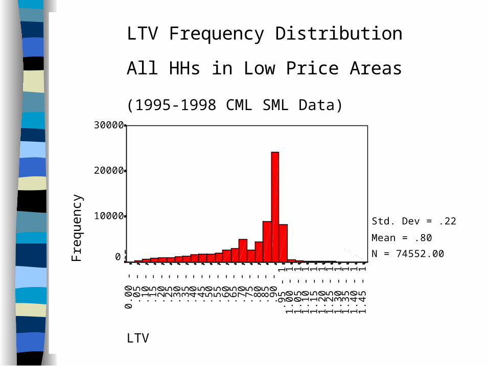
LTV Frequency Distribution
All HHs in Low Price Areas
(1995-1998 CML SML Data)
Fre
quen
cy
30000
20000
10000
0
Std. Dev = .22
Mean = .80
N = 74552.00
40LTV
.95
- 1.
00.9
0 -
.95
.85
- .9
0.8
0 -
.85
.75
- .8
0.7
0 -
.75
.65
- .7
0.6
0 -
.65
.55
- .6
0.5
0 -
.55
.45
- .5
0.4
0 -
.45
.35
- .4
0.3
0 -
.35
.25
- .3
0.2
0 -
.25
.15
- .2
0.1
0 -
.15
.05
- .1
00.
00 -
.05
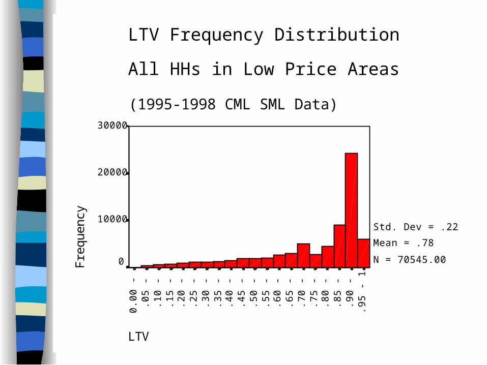
LTV Frequency Distribution
All HHs in Low Price Areas
(1995-1998 CML SML Data)
Fre
qu
en
cy
30000
20000
10000
0
Std. Dev = .22
Mean = .78
N = 70545.00
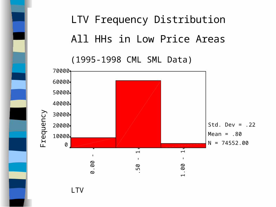
41LTV1.
00 -
1.5
0
.50
- 1.
00
0.00
- .
50
LTV Frequency Distribution
All HHs in Low Price Areas
(1995-1998 CML SML Data)
Fre
quen
cy
70000
60000
50000
40000
30000
20000
10000
0
Std. Dev = .22
Mean = .80
N = 74552.00