11

Effect of Microfinance on Vulnerability, Effect of Microfinance on Vulnerability, Poverty and Risk in Low Income Poverty and Risk in Low Income

HouseholdsHouseholds

Centre for Microfinance, IFMR, Chennai Centre for Microfinance, IFMR, Chennai 88th th January 2008January 2008

Ranjula Bali Swain Ranjula Bali Swain Department of Economics Department of Economics

Uppsala UniversityUppsala University

(co-author: Prof. Maria Floro, (co-author: Prof. Maria Floro, American University, D.C)American University, D.C)

22

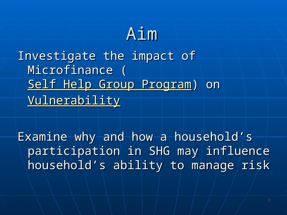
AimAimInvestigate the impact of Microfinance Investigate the impact of Microfinance

((Self Help Group ProgramSelf Help Group Program) on ) on VulnerabilityVulnerability

Examine why and how a household’s Examine why and how a household’s participation in SHG may influence participation in SHG may influence household’s ability to manage riskhousehold’s ability to manage risk

33

Theoretical formulationTheoretical formulation of effect of SHG participation: of effect of SHG participation:

1.1. Pecuniary (Pecuniary (ΠΠ) and earning effect through SHGs credit and ) and earning effect through SHGs credit and saving provision leads to increase in income (also saving provision leads to increase in income (also difference in perceived income) reflected in functiondifference in perceived income) reflected in function

2.2. Non-pecuniary effect (Non-pecuniary effect (ΞΞ) through mutual support and ) through mutual support and institutional arrangement in group and outside (difference institutional arrangement in group and outside (difference in perceived risk) , reflected in ability to cope with in perceived risk) , reflected in ability to cope with unexpected shocks defined by the subjective probability unexpected shocks defined by the subjective probability distribution of future income with mean distribution of future income with mean ξξ

Therefore, the perceived risk and perceived future Therefore, the perceived risk and perceived future earnings will cause SHG household’s probability earnings will cause SHG household’s probability distribution of future income to differ from a non-SHG distribution of future income to differ from a non-SHG membermember

44

Causes two shifts in the SHG’s probability Causes two shifts in the SHG’s probability distribution of future incomedistribution of future income

Additive shift (Additive shift (θθ) which is an increase in the ) which is an increase in the mean with all other moments constantmean with all other moments constant

Variance shift (Variance shift (γγi) by which the distribution is i) by which the distribution is more dispersed (or stretched) around zero.more dispersed (or stretched) around zero.

Holding other factors constant, we then test Holding other factors constant, we then test whether a decrease in the SHG household’s whether a decrease in the SHG household’s uncertainty leads to an increase or decrease in uncertainty leads to an increase or decrease in present consumption, and hence, a decrease or present consumption, and hence, a decrease or increase in risk coping abilityincrease in risk coping ability

5

Theoretical Framework

• Household is an economic actor that makes decision on how much risk to undertake, given its propensity to manage (ψi) – Risk Coping function is

Ri= ai + ψi Y i, i=1, 2….n households; i є S or N; (1)

and ψi ≥ 0.

Non SHG risk coping ai is the level of saving, credit and other resources available to the household i for coping which do not depend on participation in SHG

SHG risk coping ψi is the propensity of a household to deal with shock, and Yi is household income. A higher ψi reflects the household’s ability to set aside a larger portion of household income in order to cope with shock.

66

Theoretical Model explains that:

Household’s risk coping ability is affected not only by the change in earnings in a given time period, but also by the household’s perceived future earnings (Π) and perceived risk (Ξ) implying that a participation in SHG is likely to affect the household’s consumption smoothing ability and hence reduce its vulnerability.

77

Measuring VulnerabilityMeasuring Vulnerability

Unlike poverty one cannot rely on measuring household Unlike poverty one cannot rely on measuring household income or exp. Because the income or exp. Because the household welfarehousehold welfare is is presumed to depend not just on presumed to depend not just on what consumption what consumption expenditure are actually realisedexpenditure are actually realised but on but on what what consumption expenditures might beconsumption expenditures might be

Therefore Therefore measuring vulnerabilitymeasuring vulnerability involves involves twotwo steps: steps: 1.1. Estimate the Estimate the distribution of future consumption distribution of future consumption

expenditureexpenditure for all households for all households2.2. Construct a statistics from this estimated distribution, Construct a statistics from this estimated distribution,

meant to capture the meant to capture the reduction in household welfare due reduction in household welfare due to risk in household welfare to risk in household welfare resulting from the risk in the resulting from the risk in the household consumption expenditure (summarizing the household consumption expenditure (summarizing the welfare consequences of this variation)welfare consequences of this variation)

88

Three main approachesThree main approaches in literature : in literature :

1.1. Focus on responses of household consumption Focus on responses of household consumption expenditure to various observable shocks such as expenditure to various observable shocks such as drought or idiosyncratic fluctuations in incomedrought or idiosyncratic fluctuations in income

2.2. Adapt std. poverty measures to a non-deterministic Adapt std. poverty measures to a non-deterministic setting by estimating the expected value of poverty setting by estimating the expected value of poverty measuresmeasures

3.3. Utility approach to measure the welfare impact: Use von Utility approach to measure the welfare impact: Use von Neumann-Morgenstern utility functions (particularly Neumann-Morgenstern utility functions (particularly Hyperbolic Absolute Risk Aversion, HARA) to measure the Hyperbolic Absolute Risk Aversion, HARA) to measure the welfare loss associated with risk – Ligon and Schecher welfare loss associated with risk – Ligon and Schecher (2003) adopts a transformation of HARA (2003) adopts a transformation of HARA

99

Ligon and Schecher (2003) MeasureLigon and Schecher (2003) Measure

Define Vulnerability asDefine Vulnerability as

Decomposing this Vulnerability into measures of poverty and risk by taking expectations

Minimising Vulnerability is similar to maximising utilitarian social welfare function subject to aggregate resource constraints

1010

Estimating Vulnerability

• Choose the utility function

•Assume for any household probability distribution of consumption in the two period

• Step I estimate the consumption prediction equation (different from L&S because we estimate log-linear)

Use restricted least squares to estimate

•Step II these are used to construct conditional expectation

The components of Vulnerability are then regressed on household characteristics

1111

DataData Scientific Survey of the Households 2 time periods: 2000 and Scientific Survey of the Households 2 time periods: 2000 and

20032003

Quasi Experimental DesignQuasi Experimental Design

Total Sample =1025 households (SHG plus control group)Total Sample =1025 households (SHG plus control group)

Table 1: Summary Characteristics of Sample Households

2000 2003 Variable Mean value Mean value Age of Respondent 31.5 34.5 No education 65.56% 65.56% Primary education 14.24% 14.34% Secondary education 17.07% 16.78% Post-Secondary education 3.12% 3.32% Family size 4.6 4.8 Real monthly income per capita 270 338.4 No. of earners per household - 0.57 # of per capita members engaged in primary activity in the household

0.59 0.56

# of per capita members engaged as workers in the household

0.61 0.57

Cultivated land size (in acres) 1.20 1.32 Total land owned by the household (in acres) 0.86 0.96 Real value of total assets (in Rs.) 97731 124,101

1212

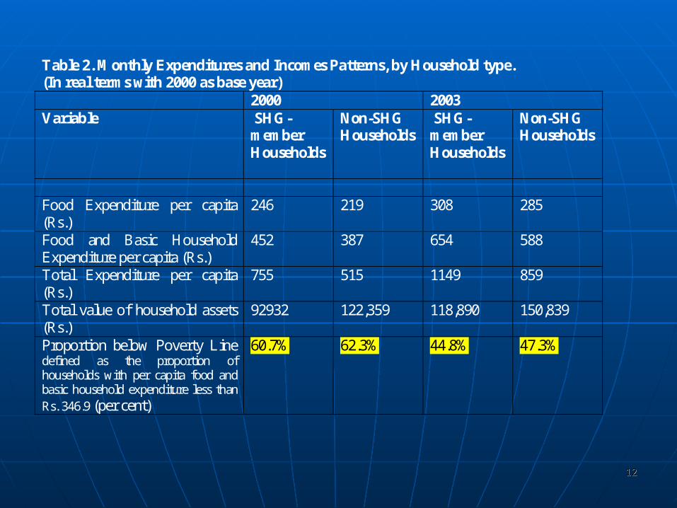
Table 2. Monthly Expenditures and Incomes Patterns, by Household type. (In real terms with 2000 as base year) 2000 2003 Variable SHG-

member Households

Non-SHG Households

SHG-member Households

Non-SHG Households

Food Expenditure per capita (Rs.)

246 219 308 285

Food and Basic Household Expenditure per capita (Rs.)

452 387 654 588

Total Expenditure per capita (Rs.)

755 515 1149 859

Total value of household assets (Rs.)

92932 122,359 118,890 150,839

Proportion below Poverty Line defined as the proportion of households with per capita food and basic household expenditure less than Rs. 346.9 (per cent)

60.7% 62.3% 44.8% 47.3%

1313

India

Survey conducted in Survey conducted in 5 states in India 5 states in India

Orissa (Koraput Orissa (Koraput and Rayagada)and Rayagada)

Andhra Pradesh Andhra Pradesh (Medak and (Medak and Rangareddy)Rangareddy)

Tamil Nadu Tamil Nadu (Dharamapuri and (Dharamapuri and Villupuram)Villupuram)

Uttar Pradesh Uttar Pradesh (Allahabad and (Allahabad and Rae Bareli)Rae Bareli)Maharashtra Maharashtra (Gadchiroli and (Gadchiroli and Chandrapur)Chandrapur)

Back to slide

1414

Table . Correlates and Decomposition of vulnerability in real per capita food and household consumption for SHG Households Av. value Vulnerability Poverty Agg. Risk Id. Risk Unexpl. Risk (in utils) .1708*** = .1312*** + .0175*** +.0012** + .0208*** [.128 , .216] [.091, .178] [.0146, .0203] [.0005, .0025] [.016, .026] Variable Coef. Coef. Coef. Coef. Coef. Sex 0.0164

(.0747) 0.0244 (.0737)

0.00021 (.00098)

-0.00061 (.0005)

-0.0077* (.0043)

Age -0.00023 (.0024)

-0.00066 (.002)

-.000017 (.000028)

.000045** (.00002)

0.00041** (.0001)

Primary .017 (.0719)

0.0198 (.0705)

.000051 (.00077)

-.000041 (.00044)

-0.00286 (.0022)

Secondary -0.259*** (.0571)

-0.2619*** (.053)

-0.003*** (.00069)

.0000019 (.00035)

0.00656 (.0047)

College edu -0.3339*** (.1214)

-0.3190*** (.1173)

-0.004*** (.0015)

-0.00147*** (.0005)

-0.0087*** (.0032)

Family size 0.104*** (.0153)

0.1010*** (.0153)

0.0012*** (.00019)

0.00024*** (.000096)

0.00113** (.00055)

Ratio of hh members that are workers

---0.119*** (.0388)

-0.1110*** (.0386)

-0.002*** (.00055)

0.00118 (.0008)

-0.0065*** (.0021)

Ratio of hh members engaged in primary activity

-0.00033 (.0568)

-0.0014 (.0548)

0.00018 (.0009)

-0.00163*** (.0004)

0.00256 (.0041)

Total land owned 0.00041 (.01453)

0.0001 (.014)

-.000016 (.00016)

-.000052 (.0001)

0.00032 (.0008)

Total cultivated land area -0.0107 (.01561)

-0.0102 (.0154)

-0.00012 (.0002)

-.000033 (.00002)

-0.00035 (.0003)

Andhra Pradesh -0.3499*** (.0530)

-0.345*** (.0520)

-0.005*** (.0008)

0.00035 (.00036)

0.00127 (.0022)

Maharastra 0.35199*** (.0683)

0.333*** (.0678)

0.0036*** (.0008)

0.00048 (.0004)

0.0135*** (.0036)

Tamil Nadu 0.0196 (.0644)

0.0072 (.0631)

-0.0003 (.0008)

0.00035 (.0004)

0.0124*** (.0045)

Orissa 0.2730** (.0622)

0.2560*** (.0602)

0.0034*** (.0007)

-.0001 (.0004)

0.0132*** (.0025)

Constant -0.2310* (.1338)

-0.2479* (.1288)

0.0137*** (.0019)

-0.00049 (.0011)

0.00402 (.007)

R2 .31 .31 .37 .08 .06 * Numbers in parenthesis are bootstrapped standard errors, and those in brackets are 95% confidence intervals. ***- significant at 1% level, **- significant at the 5% level and *- significant at 1% level. Uttar Pradesh is the regional default dummy.

1515

Table 4. Correlates and Decomposition of vulnerability in real per capita food and household consumption for NON-SHG households Av. value Vulnerability Poverty Agg. Risk Id. Risk Unexpl. Risk (in utils) .217*** = .175*** + .019*** +.0015 + .022*** [.126 , .326] [.0817, .28] [.013, .026] [.00012, .0048] [.0141, .0319] Variable Coef. Coef. Coef. Coef. Coef. Sex

-0.202 (.2244)

-0.208 (.2153)

-0.0028 (.0024)

.000047 (.0027)

0.00851 (.0086)

Age -0.0105** (.0045)

-0.010** (.0045)

-0.0001* (.00006)

.000019 (.00008)

-.000075 (.0004)

Primary 0.0984 (.1196)

0.0961 (.1136)

0.0016 (.0017)

-0.0004 (.00092)

0.001 (.0067)

Secondary -0.0134 (.1185)

-0.006 (.1151)

.000054 (.0016)

-0.0002 (.0016)

-0.006 (.0062)

College edu -0.560** (.2613)

-0.538** (.2585)

-0.0085** (.0035)

-0.0034** (.0016)

-0.009 (.0108)

Family size 0.115*** (.0367)

0.1129*** (.0352)

0.0012** (.0005)

-0.0001 (.0004)

0.001 (.0019)

Ratio of hh members that are workers

-0.017 (.2183)

-0.0206 (.2120)

-0.0004 (.0027)

-0.0002 (.0027)

0.003 (.0087)

Ratio of hh members that are engaged in primary activity

-0.197 (.2275)

-0.1829 (.2285)

-0.0032 (.0028)

-0.003*** (.0015)

-0.007 (.0066)

Total land owned -0.064 (.0920)

-0.0623 (.0919)

-0.0007 (.0011)

-.000073 (.0007)

-0.001 (.0037)

Total cultivated land area

0.007 (.0788)

0.0068 (.0771)

0.0001 (.0009)

.000044 (.0007)

0.0003 (.0043)

Andhra Pradesh -0.529*** (.1285)

-0.523*** (.1265)

-0.008*** (.0019)

-0.001 (.0015)

0.002 (.013)

Maharastra 0.061 (.1214)

0.0531 (.1657)

0.0003 (.0019)

-0.0004 (.0018)

0.008 (.0085)

Tamil Nadu -0.202* (.1214)

-0.199 (1216)

-0.0036** (.0015)

-0.0019* (.0011)

0.001 (.0077)

Orissa 0.284** (.1372)

0.270*** (.1341)

0.0031* (.0017)

-0.0003 (.0020)

0.01 (.0091)

Constant 0.404 (.3346)

0.367 (.3280)

0.0227*** (.0057)

0.0051 (.0065)

0.009 (.0195)

R2 .35 .34 .40 .13 .04 Numbers in brackets are 99% confidence intervals. ***- significant at 1% level, **- significant at the 5% level and *- significant at 1% level. Uttar Pradesh is the regional default dummy.

1616

Table 5. Percentage contribution to the total vulnerability for model and (in percent)

SHG Households Non-SHG households

Poverty component of vulnerability 76.8% 80.6%

Aggregate risk 10.2% 8.7%

Idiosyncharactic risk 0.7% .7%

Unexplained risk 12.1% 10.1%

1717

ConclusionsConclusions

Vulnerability lower in SHGs as Vulnerability lower in SHGs as compared to control groups compared to control groups

Main component of vulnerability is Main component of vulnerability is from poverty; aggregate risk is also from poverty; aggregate risk is also importantimportant

Microfinance (SHG) leads to decrease Microfinance (SHG) leads to decrease in vulnerabilityin vulnerability

1818

Thank you for your attention!

Ranjula.Bali@nek.uu.se

1919

Self Help Bank Linkage ProgramSelf Help Bank Linkage ProgramTable. Information on Self Help Groups A. Physical Achievements 1.Number of poor families who have accessed bank credit up to March 2005

24.3 million

2. Estimated number of poor people assisted up to March 2005 121.5 million 3. Percentage of SHGs comprised of women 90 4. Cumulative number of SHGs financed by banks up to March 2005

1,618,456

B. Financial Results 1. Cumulative bank loans disbursed to SHGs up to March 2005 More than Rs.68 billion** 2. Bank loans disbursed to new SHGs during 2004-2005 Rs. 17,266 million 3. Increase in credit flow to SHGs over the previous year 61% 4. On-time repayment reported by participating banks Over 95 per cent Partnerships 1. Number of participating banks 573 2. Commercial banks 47 3. Regional Rural Banks (RRBs) 196 4. Cooperatives 330 5. Number of bank branches lending to SHGs 41,082 6. Number of participating NGO and other agencies 4,323

2020

Self Help Group (SHG) ProgramSelf Help Group (SHG) Program

Group of about 15 people from a homogenous class Group of about 15 people from a homogenous class - financial discipline through self savings and - financial discipline through self savings and lending within the group initially.lending within the group initially.

When group demonstrates this mature financial When group demonstrates this mature financial behaviour banks are encouraged to make loans - behaviour banks are encouraged to make loans - peer pressure ensures timely repayments NABARD, peer pressure ensures timely repayments NABARD, 2005.2005.

use of the existing and extensive infrastructure of use of the existing and extensive infrastructure of rural bank branches for disbursing microfinance rural bank branches for disbursing microfinance services –refinancing by NABARD, linked to groups services –refinancing by NABARD, linked to groups through commercial banks, NGOs etc.through commercial banks, NGOs etc.

Government also implementing poverty alleviation Government also implementing poverty alleviation programs through SHGsprograms through SHGs

Back

2121

VulnerabilityVulnerability

Household’s sense of well-being depends not Household’s sense of well-being depends not just on its average income or expenditure just on its average income or expenditure (poverty) but the risk it faces- particularly (poverty) but the risk it faces- particularly important for low-income/resource important for low-income/resource householdshouseholds

We define it as the household and its members’ ability to deal with risks, shocks and proneness to food security and hence their attitude towards undertaking risks.

Back