1

Economics 331b

Treatment of Uncertaintyin Economics (II)

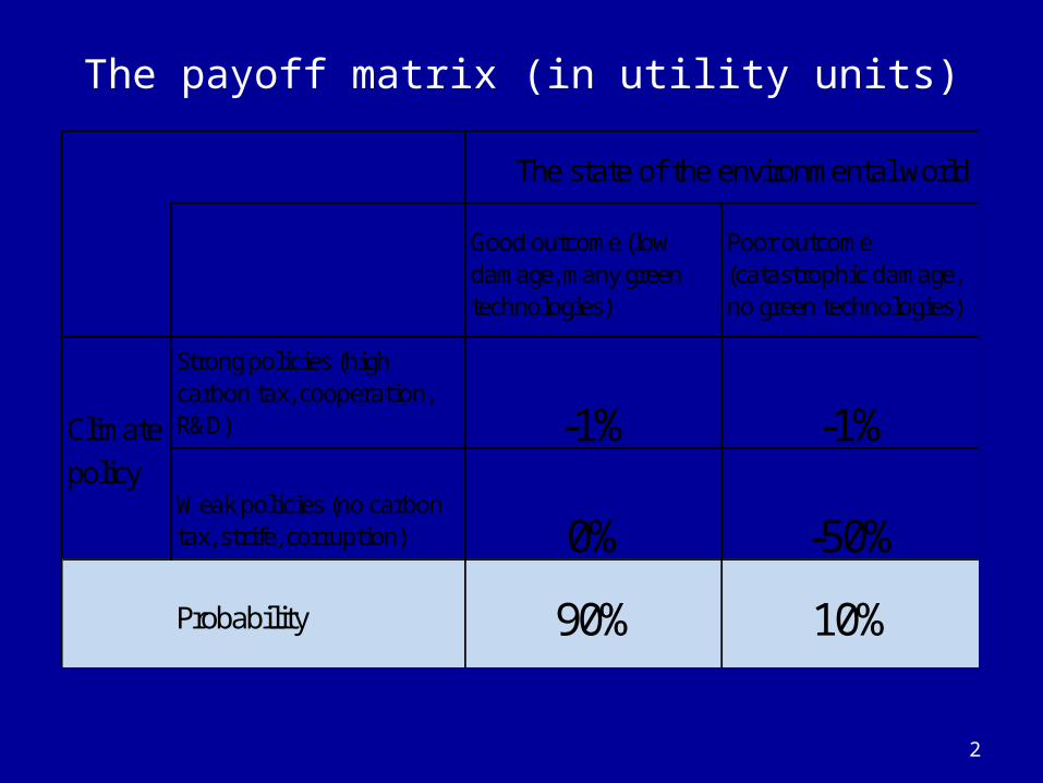
The payoff matrix (in utility units)

2

The state of the environmental world

Good outcome (low damage, many green technologies)

Poor outcome (catastrophic damage, no green technologies)

Climate

Strong policies (high carbon tax, cooperation, R&D) -1% -1%

policyWeak policies (no carbon tax, strife, corruption) 0% -50%

Probability 90% 10%

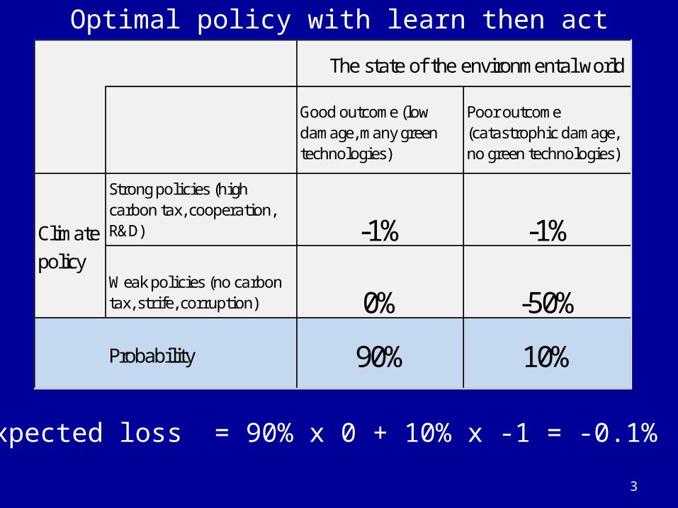
Optimal policy with learn then act

3

The state of the environmental world

Good outcome (low damage, many green technologies)

Poor outcome (catastrophic damage, no green technologies)

Climate

Strong policies (high carbon tax, cooperation, R&D) -1% -1%

policyWeak policies (no carbon tax, strife, corruption) 0% -50%

Probability 90% 10%

Expected loss = 90% x 0 + 10% x -1 = -0.1%

ACT in future

High damages

High carbon tax

Low carbon taxLow damages

This example: Learn then act

LEARNTODAY

What is wrong with this story?

The Monte Carlo approach is “learn then act.”That is, we learn the role of the dice, then we adopt

the best policy for that role.But this assumes that we know the future!

- If you know the future and decide (learn then act)- If you have to make your choice and then live with

the future as it unfolds (act then learn)

In many problems (such as climate change), you must decide NOW and learn about the state of the world LATER: “act then learn”

5

Decision Analysis

In reality, we do not know future trajectory or SOW (“state of the world”).

Suppose that through dedicated research, we will learn the exact answer in 50 years.

It means that we must set policy now for both SOW; we can make state-contingent policies after 50 years.

How will that affect our optimal policy?

6

LEARN 2050ACT

TODAY?

Low damages

High damages

Realistic world:Act then learn

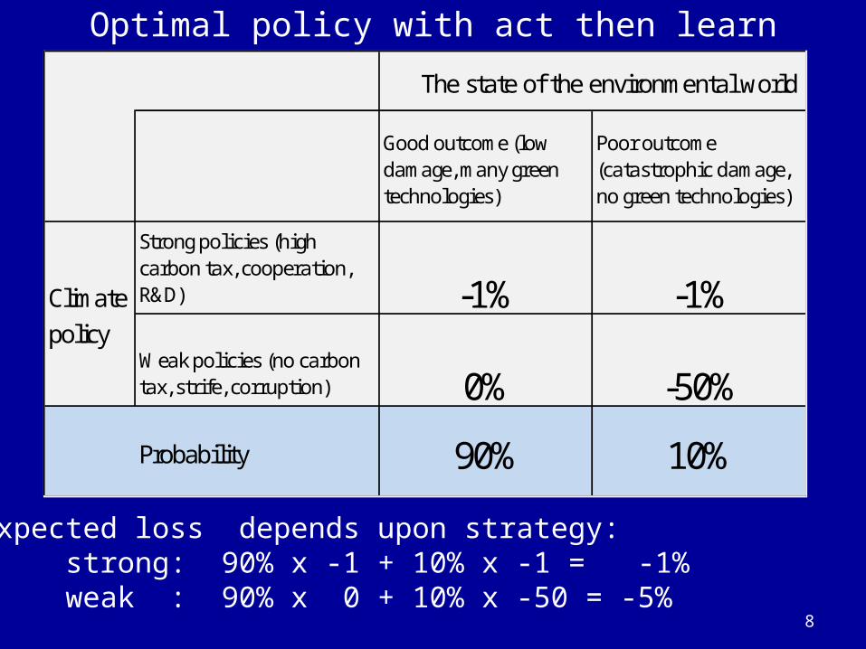
Optimal policy with act then learn

8

The state of the environmental world

Good outcome (low damage, many green technologies)

Poor outcome (catastrophic damage, no green technologies)

Climate

Strong policies (high carbon tax, cooperation, R&D) -1% -1%

policyWeak policies (no carbon tax, strife, corruption) 0% -50%

Probability 90% 10%

Expected loss depends upon strategy:strong: 90% x -1 + 10% x -1 = -1%weak : 90% x 0 + 10% x -50 = -5%

Conclusions

When you have learning, the structure of decision making is very different; it can increase of decrease early investments.

In cases where there are major catastrophic damages, value of early information is very high. Best investment is sometimes knowledge rather than

mitigation (that’s why we are here!)

9

10

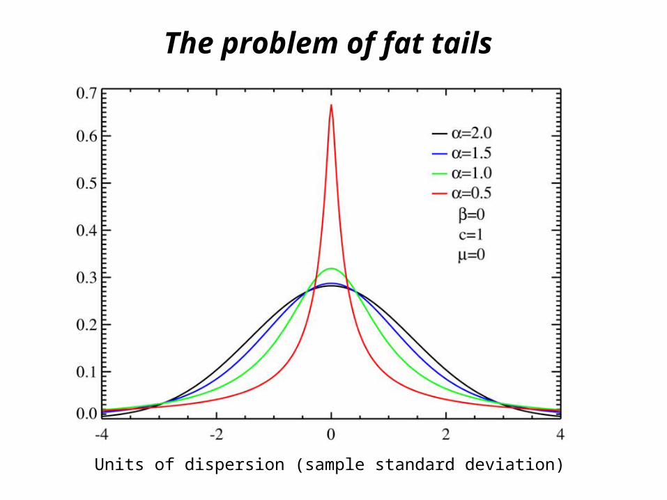
The problem of fat tails

Units of dispersion (sample standard deviation)

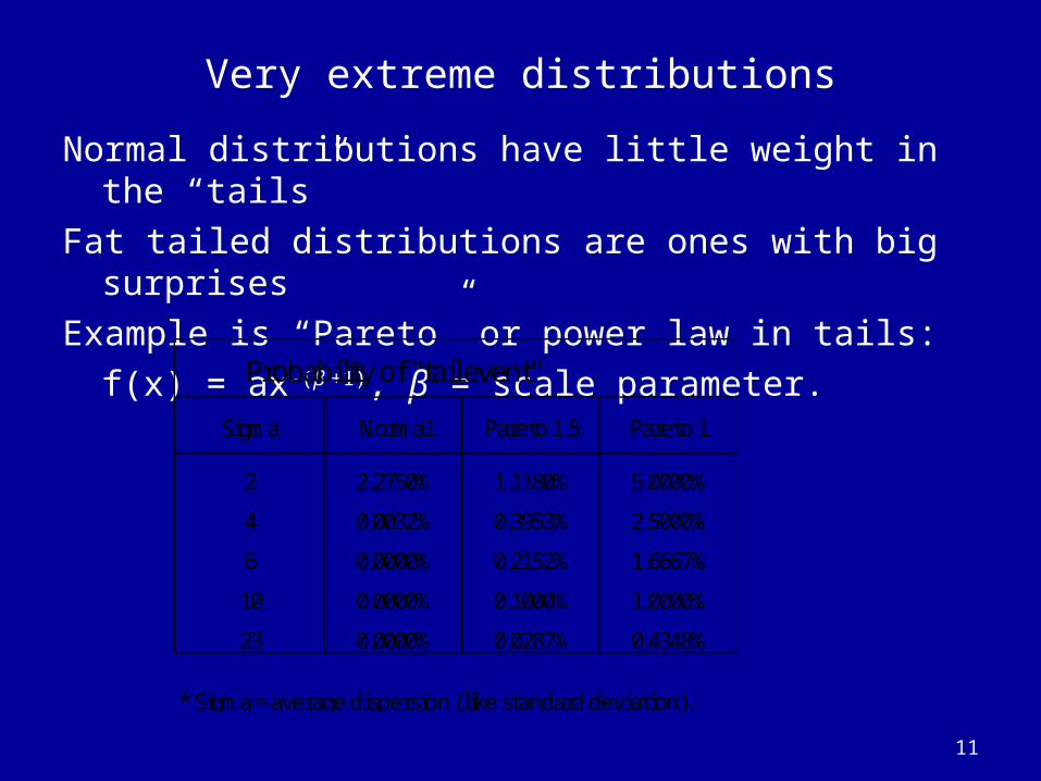
Very extreme distributions

Normal distributions have little weight in the “tails”Fat tailed distributions are ones with big surprisesExample is “Pareto” or power law in tails:

f(x) = ax-(β +1), β = scale parameter.

11

Probability of "tail event"

Sigma Normal Pareto 1.5 Pareto 1

2 2.2750% 1.1180% 5.0000%

4 0.0032% 0.3953% 2.5000%

6 0.0000% 0.2152% 1.6667%

10 0.0000% 0.1000% 1.0000%

23 0.0000% 0.0287% 0.4348%

* Sigma = average dispersion (like standard deviation).

12

Black swans in South Africa (“Birds of Eden”)

Some examples

Height of American women: Normal N(64”,3”).

How surprised would you be to see a 14’ person coming to Econ 331?

13

Some examples

Stock market: what is the probability of a 23% change in one day for a normal distribution? Circa 10-230 !!!- Mandelbrot found it was Pareto with β= 1.5.- Finite mean, but infinite variance

Earthquakes: Cauchy distribution β = 1 (see next slide). - Infinite mean, infinite variance

14

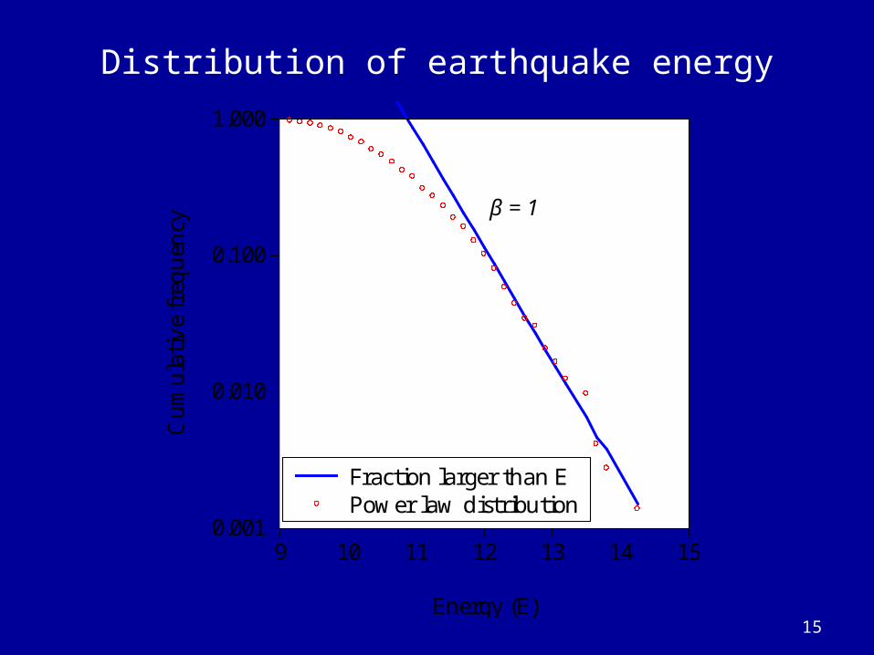
Distribution of earthquake energy

15

1.000

0.100

0.010

0.0019 10 11 12 13 14 15

Energy (E)

Fraction larger than EPower law distribution

Cum

ula

tive

freq

uen

cy

β = 1

Surprise with fat tails

Suppose you were a Japanese planner and used historical earthquakes as your guidelines.

How surprised were you in March 2011? How much more energy in that earthquake that LARGEST in all of Japanese history?

Answer:(9.0/8.5)^10 ^1.5= 5.6 times as large as historical max.

16

Some examples

Climate damages (fat tailed according to Weitzman, but ?)

17

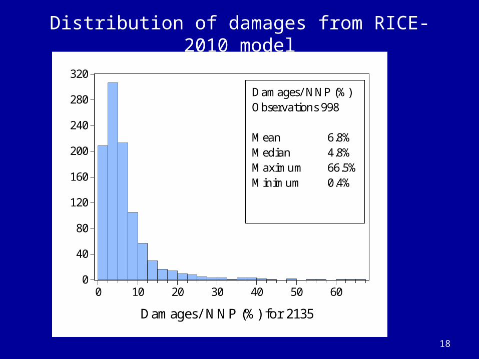
Distribution of damages from RICE-2010 model

18

0

40

80

120

160

200

240

280

320

0 10 20 30 40 50 60

Damages/ NNP (%)Observations 998

Mean 6.8%Median 4.8%Maximum 66.5%Minimum 0.4%

Damages/ NNP (%) for 2135

Here is another motivation: surprise

Fat tailed distributions are ones that are very surprising if you just look at historical data.

Suppose you were an oil trader in the late 1960s and early 1970s.

You are selling “vols” (volatility options).Let’s rerun history.

19

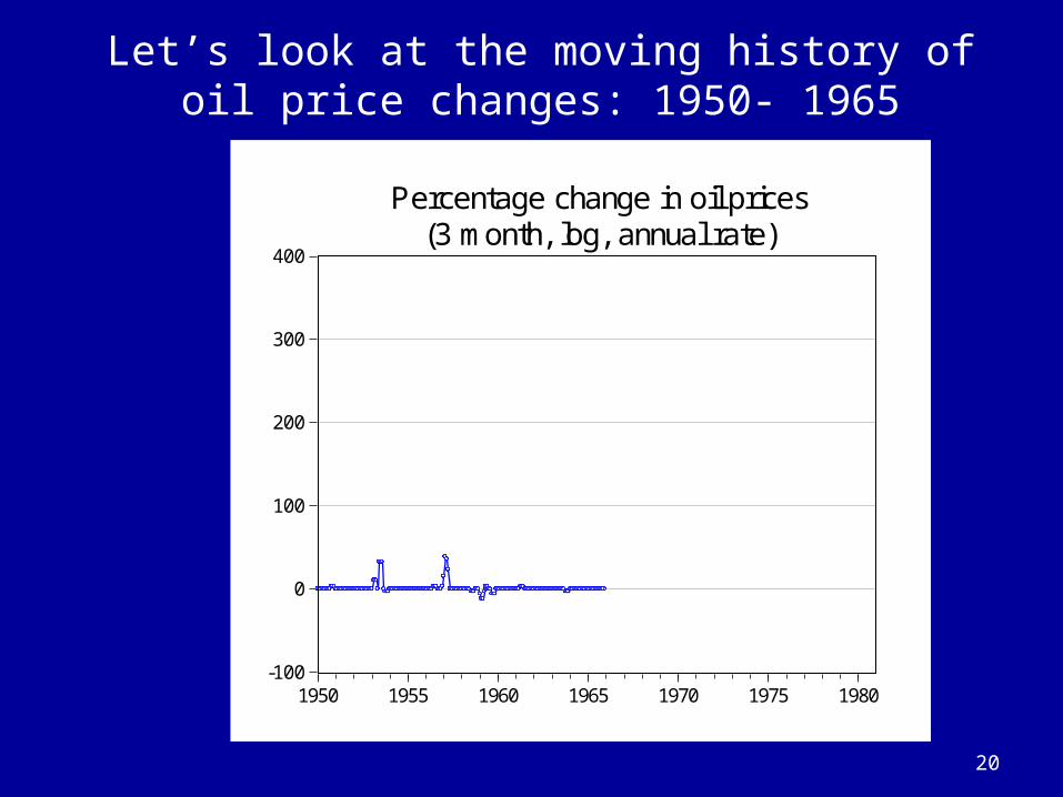
Let’s look at the moving history of oil price changes: 1950- 1965

20

-100

0

100

200

300

400

1950 1955 1960 1965 1970 1975 1980

Percentage change in oil prices(3 month, log, annual rate)

Oil price changes: 1950- 1970

21

-100

0

100

200

300

400

1950 1955 1960 1965 1970 1975 1980

Percentage change in oil prices(3 month, log, annual rate)

Oil price changes : 1950- 1973:6

22

-100

0

100

200

300

400

1950 1955 1960 1965 1970 1975 1980

Percentage change in oil prices(3 month, log, annual rate)

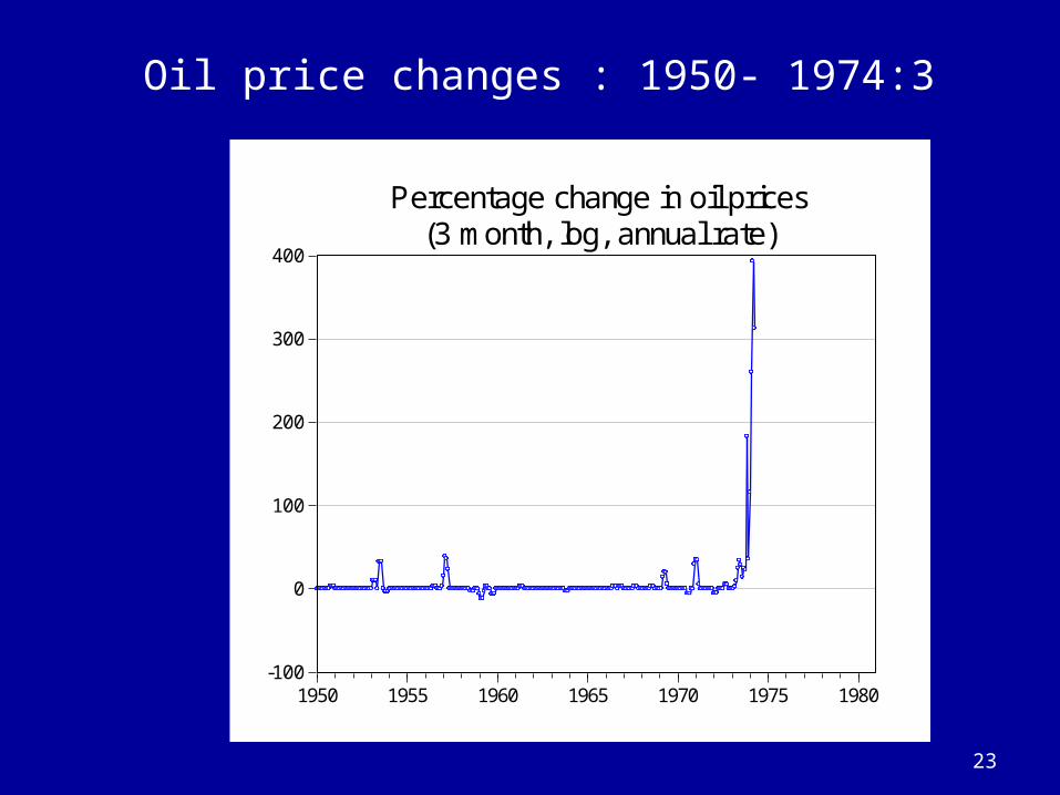
Oil price changes : 1950- 1974:3

23

-100

0

100

200

300

400

1950 1955 1960 1965 1970 1975 1980

Percentage change in oil prices(3 month, log, annual rate)

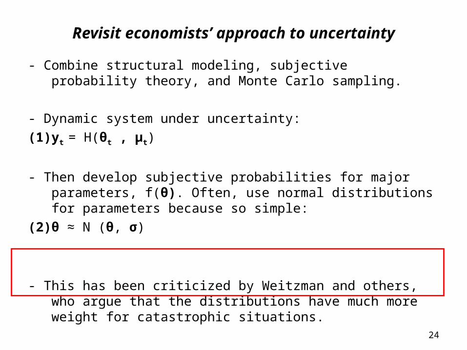
Revisit economists’ approach to uncertainty

- Combine structural modeling, subjective probability theory, and Monte Carlo sampling.

- Dynamic system under uncertainty:(1) yt = H(θt , μt)

- Then develop subjective probabilities for major parameters, f(θ). Often, use normal distributions for parameters because so simple:

(2) θ ≈ N (θ, σ)

- This has been criticized by Weitzman and others, who argue that the distributions have much more weight for catastrophic situations.

24

Weitzman’s contribution

Weitzman showed that with fat tailed distribution, might have negative infinite utility, and no optimal policy.

25

Some technicalia on Weitzman Critique

Weitzman argues that IAMs have ignored the “fat tailed” nature of probability distributions. If these are considered, then may get very different results. (Rev. Econ. Stat, forth. 2009)

Weitzman’s definition of fat tails is unbounded moment generating function:

Note that this is unusual both substantively and because it involves preferences (CRRA parameter, α ).

Combine the CRRA utility with Pareto distribution (β) for consumption.

Dismal Theorem: Have real problems is α is too high or β is too small.

26

- c

c=0

E(c)= e f(c)dc=-∞

∞

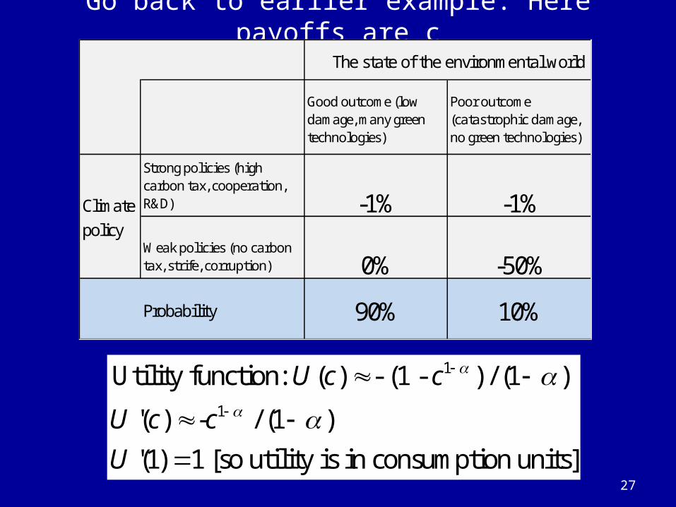
Go back to earlier example. Here payoffs are c

27

The state of the environmental world

Good outcome (low damage, many green technologies)

Poor outcome (catastrophic damage, no green technologies)

Climate

Strong policies (high carbon tax, cooperation, R&D) -1% -1%

policyWeak policies (no carbon tax, strife, corruption) 0% -50%

Probability 90% 10%

1

1

Utility function: ( ) - (1 - ) / (1 )

'( ) - / (1 )

'(1) 1 [so utility is in consumption units]

U c c

U c c

U

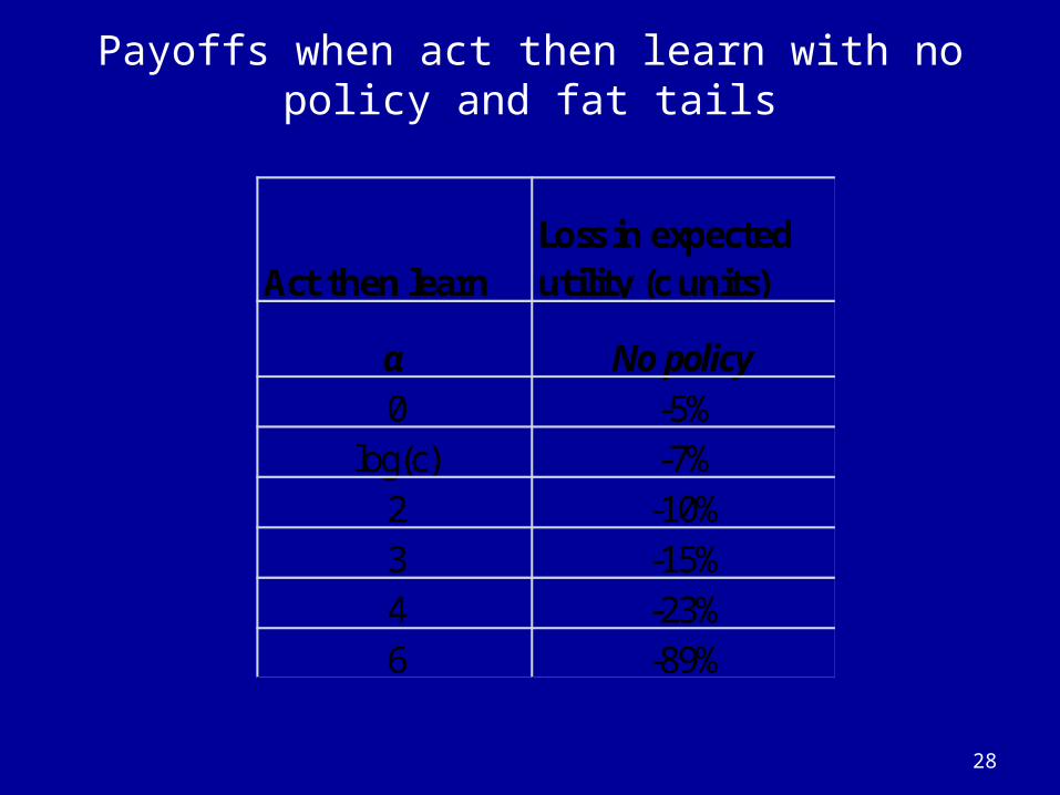
Payoffs when act then learn with no policy and fat tails

28

Act then learnLoss in expected utility (c units)

α No policy0 -5%

log(c) -7%2 -10%3 -15%4 -23%6 -89%

Payoffs when have policy, act then learn

29

Act then learn Loss in expected utility (c units)

α Weak policy Strong policy0 -5.00% -1.00%

1.01 -6.96% -1.01%2 -10.00% -1.01%3 -15.00% -1.02%4 -23.33% -1.02%6 -89.45% -1.03%

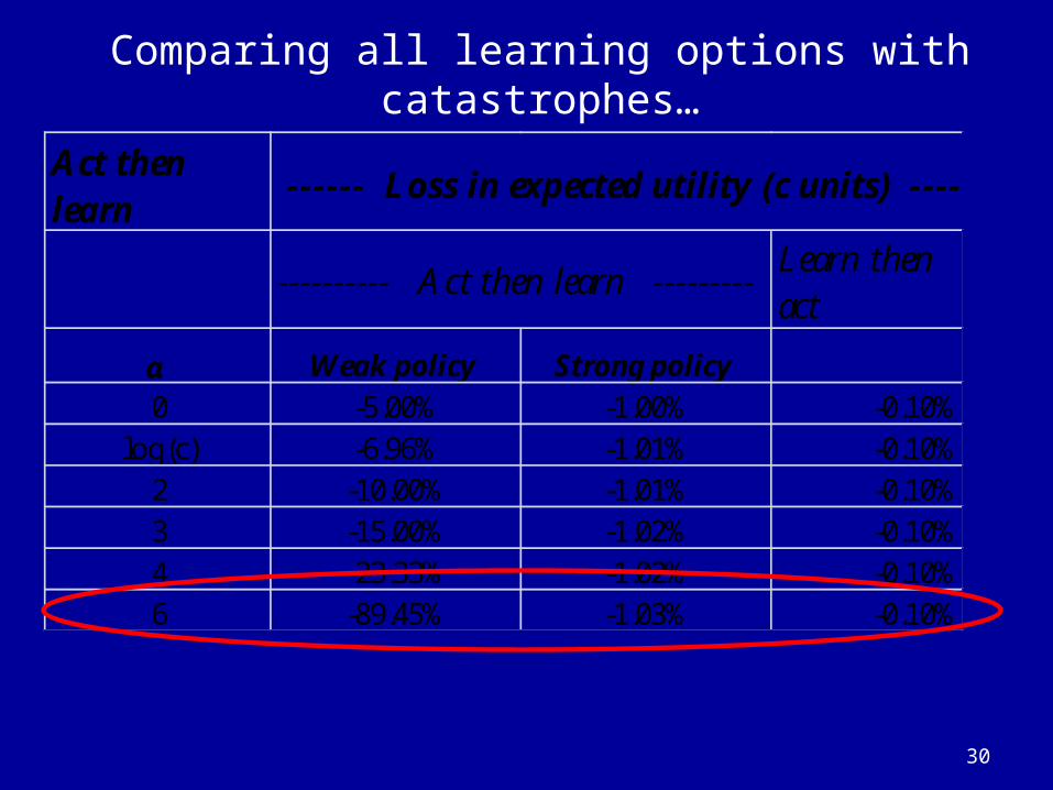
Comparing all learning options with catastrophes…

30

Act then learn

------ Loss in expected utility (c units) ----

---------- Act then learn ---------Learn then act

α Weak policy Strong policy0 -5.00% -1.00% -0.10%

log(c) -6.96% -1.01% -0.10%2 -10.00% -1.01% -0.10%3 -15.00% -1.02% -0.10%4 -23.33% -1.02% -0.10%6 -89.45% -1.03% -0.10%

Conclusions on fat tails

1. Fat tails are very fun (unless you get caught in a tsunami).

2. Fat tails definitely complicate life and losses.- Particularly with power law (Pareto) with low β.

3. Fat tails are particularly severe if we act stupidly. - Drive 90 mph while drunk, text messaging, on ice

roads.

4. If have good policy options, can avert most problems of fat tails.

5. If have early learning, can do even better.

31