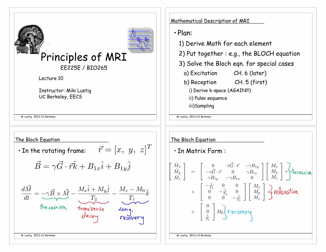
M. Lustig, EECS UC Berkeley

Principles of MRIEE225E / BIO265

Lecture 10

Instructor: Miki LustigUC Berkeley, EECS

M. Lustig, EECS UC Berkeley

Mathematical Description of MRI

• Plan:1) Derive Math for each element2) Put together : e.g., the BLOCH equation3) Solve the Bloch eqn. for special cases

a) Excitation CH. 6 (later)b) Reception CH. 5 (first)

i) Derive k-space (AGAIN!!!)ii) Pulse sequenceiii)Sampling

M. Lustig, EECS UC Berkeley

The Bloch Equation

• In the rotating frame:

d ~M

dt= �� ~B ⇥ ~M � M

x

i+My

j

T2� M

z

�M0

T1k

~r = [x, y, z]T

~B = � ~G · ~rk +B1xi+B1y j

M. Lustig, EECS UC Berkeley

The Bloch Equation

• In Matrix Form :2

4M

x

My

Mz

3

5 =

2

40 � ~G · ~r ��B1y

�� ~G · ~r 0 �B1x

�B1y ��B1x 0

3

5

2

4M

x

My

Mz

3

5+

+

2

4� 1

T20 0

0 � 1T2

00 0 � 1

T1

3

5

2

4M

x

My

Mz

3

5+

+

2

4001T1

3

5M0

M. Lustig, EECS UC Berkeley

Bloch Equation

• Combined (rotating frame)

• T1 is the source of all signals!• Magnetization distribution unknown• Can probe by changing B1 and G

2

4M

x

My

Mz

3

5 =

2

64� 1

T2� ~G · ~r ��B1y

�� ~G · ~r � 1T2

�B1x

�B1y ��B1x � 1T1

3

75

2

4M

x

My

Mz

3

5+

2

4001T1

3

5M0

M. Lustig, EECS UC Berkeley

Solving the Bloch Equation

Two Special Cases:• Reception

– Data acquisition– Spatial encoding– Explicit solutions! (Today)

• Excitation– Non linear problems– No general solution– Many solutions for special cases (Ch. 6)

B1x = 0, B1y = 0

B1x 6= 0, B1y 6= 0

M. Lustig, EECS UC Berkeley

Reception

• Magnetization is a function of and t.Also, assume single, constant T1 and T2.

• We would like to resolve this using a time varying gradient

~r

~M(~r, t) =h~Mx

(~r, t), ~My

(~r, t), ~Mz

(~r, t)iT

~G(t) = [Gx

(t), Gy

(t), Gz

(t)]T

2

4M

x

My

Mz

3

5 =

2

64� 1

T2� ~G · ~r 0

�� ~G · ~r � 1T2

00 0 � 1

T1

3

75

2

4M

x

My

Mz

3

5+

2

4001T1

3

5M0

M. Lustig, EECS UC Berkeley

Reception

• With no B1(t) :

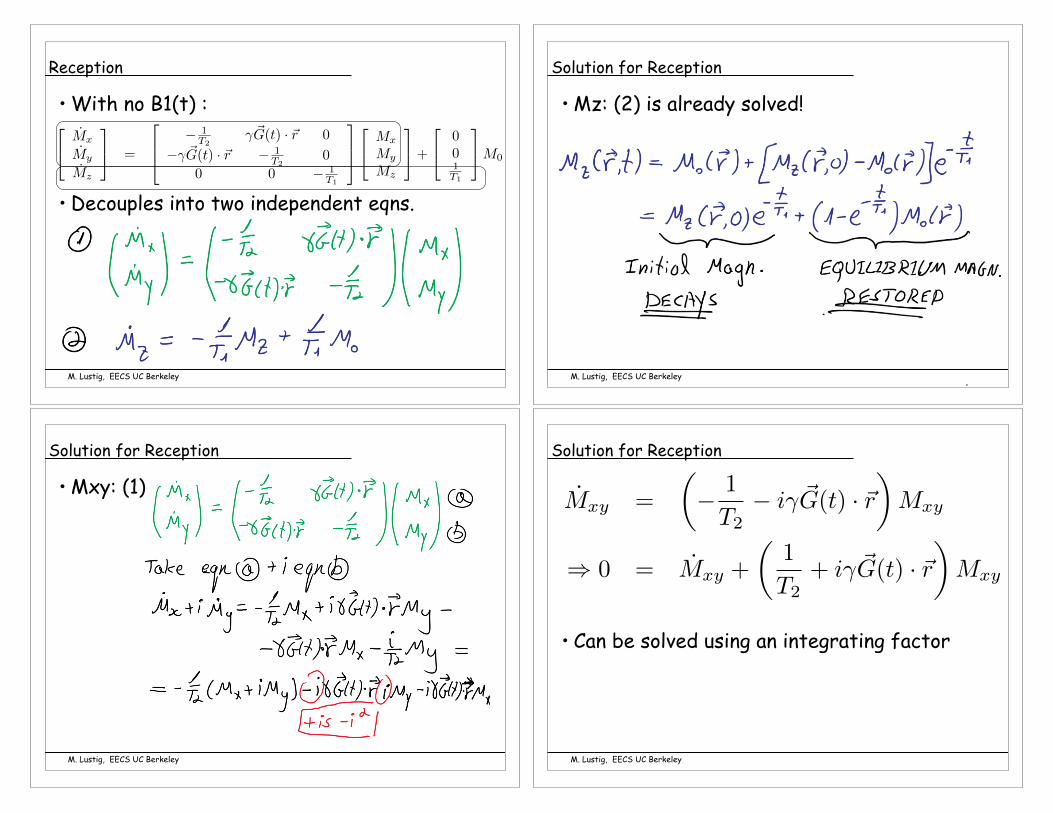
• With no B1(t) :

• Decouples into two independent eqns.

2

4M

x

My

Mz

3

5 =

2

64� 1

T2� ~G(t) · ~r 0

�� ~G(t) · ~r � 1T2

00 0 � 1

T1

3

75

2

4M

x

My

Mz

3

5+

2

4001T1

3

5M0

M. Lustig, EECS UC Berkeley

Reception

M. Lustig, EECS UC Berkeley

Solution for Reception

• Mz: (2) is already solved!

M. Lustig, EECS UC Berkeley

Solution for Reception

• Mxy: (1)M

xy

=

✓� 1

T2� i� ~G(t) · ~r

◆M

xy

) 0 = Mxy

+

✓1

T2+ i� ~G(t) · ~r

◆M

xy

M. Lustig, EECS UC Berkeley

Solution for Reception

• Can be solved using an integrating factor

y(x)M(x) =

ZQ(x)M(x) + C

M. Lustig, EECS UC Berkeley

Differential Equations 101

• Given an ODE

• Multiply with integrating factor M(x)

• So,

• And,

y

0 + p(x)y = Q(x)

M(x)y0 +M(x)p(x)y = M(x)Q(x)

(M(x)y)0 = M(x)Q(x)

Mxy

=

✓� 1

T2� i� ~G(t) · ~r

◆M

xy

) 0 = Mxy

+

✓1

T2+ i� ~G(t) · ~r

◆M

xy

M. Lustig, EECS UC Berkeley

Solution for Reception

• Can be solved using an integrating factor

et

T2+i�~r·

R t0

~G(⌧)d⌧

Mxy

+

✓1

T2+ i� ~G(t) · ~r

◆M

xy

= 0

M. Lustig, EECS UC Berkeley

Solution for Reception

• Integrate:

Mxy

(~r, t)et

T2+i�~r·

R t0

~

G(⌧)d⌧ = Mxy

(~r, 0)

⇣M

xy

et

T2+i�~r·

R t0

~

G(⌧)d⌧⌘0

= 0

Mxy

(~r, t) = Mxy

(~r, 0)e�t

T2 e�i~r·R t0 �

~

G(⌧)d⌧

~k(t) =�

2⇡

Z t

0

~G(⌧)d⌧

M. Lustig, EECS UC Berkeley

Solution for Reception

• Define a Spatial frequency vector:~k(t) = [k

x

(t), ky

(t), kz

(t)]T

M. Lustig, EECS UC Berkeley

Solution for Reception

• Transverse Magnetization Mxy is then:

• Received Signal is proportional to Mxy integrated over volume:

Mxy

(~r, t) = Mxy

(~r, 0)e�t

T2 e�i2⇡~k(t)·~r

Fourier kernel

s(t) =

Z

~

R

Mxy

(~r, 0)e�t

T2 e�i2⇡~k(t)·~rd~r

Also a function of r!M. Lustig, EECS UC Berkeley

Signal Equation

• Assume that T2 is LARGE

• So,

s(t) =

Z

~

R

Mxy

(~r, 0)e�i2⇡~k(t)·~rd~r

M. Lustig, EECS UC Berkeley

k-Space

M. Lustig, EECS UC Berkeley

k-Space Trajectories

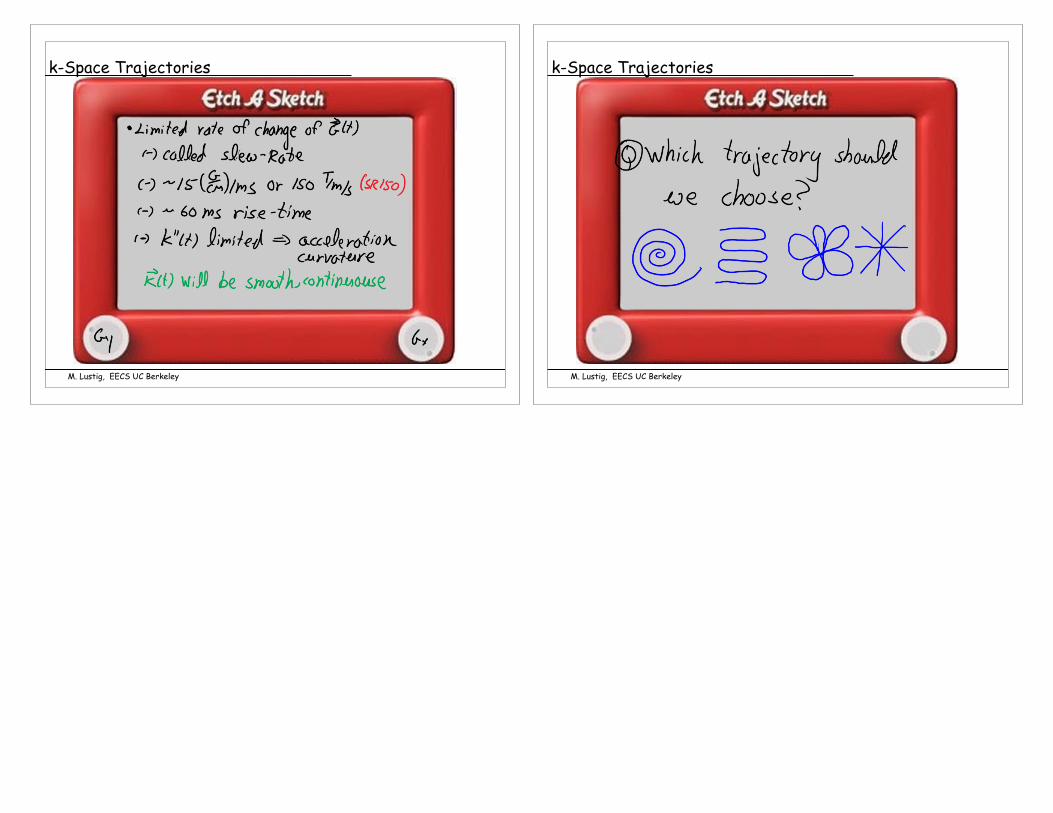
M. Lustig, EECS UC Berkeley

k-Space Trajectories

M. Lustig, EECS UC Berkeley

k-Space Trajectories