1

Data Fusion and Multi-Cue Data Matching byDiffusion Maps

Stéphane Lafon1, Yosi Keller2 and Ronald R. Coifman2

Abstract

Data fusion and multi-cue data matching are fundamental tasks of high-dimensional data analysis. In thispaper, we apply the recently introduced diffusion framework to address these tasks. Our contribution is three-fold.First, we present the Laplace-Beltrami approach for computing density invariant embeddings which are essentialfor integrating different sources of data. Second, we describe a refinement of the Nyström extension algorithmcalled “geometric harmonics”. We also explain how to use this tool for data assimilation. Finally, we introduce amulti-cue data matching scheme based on nonlinear spectral graphs alignment. The effectiveness of the presentedschemes is validated by applying it to the problems of lip-reading and image sequence alignment.

Index Terms

Pattern matching, graph theory, graph algorithms, Markov processes, machine learning, data mining, imagedatabases.

I. I NTRODUCTION

The processing of massive high-dimensional data sets is a contemporary challenge. Suppose that asources produces high-dimensional datax1, ..., xn that we wish to analyze. For instance, each datapoint could be the frames of a movie produced by a digital camera, or the pixels of a hyperspectral image.When dealing with this type of data, the high-dimensionality is an obstacle for any efficient processing ofthe data. Indeed, many classical data processing algorithms have a computational complexity that growsexponentially with the dimension (this is the so-called “curse of dimensionality”). On the other hand, thesources may only enjoy a limited number of degrees of freedom. This means that most of the variablesthat describe each data points are highly correlated, at least locally, or equivalently, that the data set has alow intrinsic dimensionality. In this case, the high-dimensional representation of the data is an unfortunate(but often unavoidable) artifact of the choice of sensors or the acquisition device. Therefore it should bepossible to obtain low-dimensional representations of the samples. Note that since the correlation betweenvariables might only be local, classical global dimension reduction methods like Principal ComponentAnalysis and Multidimensional Scaling do not provide, in general, an efficient dimension reduction.

First introduced in the context of manifold learning, eigenmaps techniques [1], [2], [3], [4] are becomingincreasingly popular as they overcome this problem. Indeed, they allow one to perform a nonlinearreduction of the dimension by providing a parametrization of the data set that preserves neighborhoods.However, the new representation that one obtains is highly sensitive to the way the data points wereoriginally sampled. More precisely, if the data are assumed to approximately lie on a manifold, then theeigenmap representation depends on the density of the points on this manifold [5]. This issue is of criticalimportance in applications as one often needs tomerge datathat were produced by the same source butacquired with different devices or sensors, at various sampling rates and possibly on different occasions. Inthat case, it is necessary to have a canonical representation of the data that retains the intrinsic constraintsof the samples (e.g. manifold geometry) regardless of the particular distribution of the datasets sampledby different devices.

1Google Inc., stephane.lafon@gmail.com2Department of Mathematics, Yale University, yosi.keller, coifman-ronald@yale.edu.

2

Another important issue is that ofdata matching. This question arises when one needs to establish acorrespondence between two data sets resulting from the same fundamental source. For instance, considerthe problem of matching pixels of a stereo image pair. One can form a graph for each image, where pixelsconstitute the nodes, and where edges are weighted according to the local features in the image. Theproblem now boils down to matching nodes between two graphs. Note that this situation is an instance ofmulti-sensor integration problem, in which one needs to find the correspondence between data captured bydifferent sensors. In some applications, like fraud detection, synchronizing data sets is used for detectingdiscrepancies rather than similarities between data sets.

The out-of-sample extension problem is another aspect of the data fusion problem. The idea is to extenda function known on a training set to a new point using both the target function and the geometry ofthe training domain. The new point and the corresponding value of the function can then be assimilatedto the training set. This is an essential component in any scheme that agglomerates knowledge over aninitial data set and then applies the inferred structure to new data. Recently, Belkinet al have developeda solution to this problem via the concept of manifold regularization [6]. Earlier, several authors usedthe Nyström extension procedure in the Machine Learning context [7], [8] in order to extend eigenmapcoordinates. In both cases, the question of the scale of the extension kernel remains unanswered. In otherwords, given an empirical function on a data set, to what distance to the training set can this functionbe extended ? In particular, given the spectral embedding of the data set, which kernel should be used toextend it?

By relating the frequency content of the target function on the training set to the extrinsic Fourieranalysis, Coifmanet al provide an answer to this question [9]. They developed the idea of “geometricharmonics” based on the Nyström extension at different scales, providing a multiscale extension schemefor empirical functions. We apply this concept to the extension of spectral embeddings and show that theextension has to be conducted using a specially designed kernel which differs from the eigenmap kernel.

In this article, we show that the questions discussed above can be efficiently addressed by the generaldiffusion framework introduced in [5], [10], [11]. The main idea is that, just like for eigenmaps methods,eigenvectors of Markov matrices can be used to embed any graph into a Euclidean space and achievedimension reduction. Building on these ideas, the contribution of this paper is three-fold:

• First, we show that by carefully normalizing the Markov matrix, the embedding can be made invariantto the density of the sampled data points, thus solving the problem of data fusion encountered withother eigenmaps methods.

• Then, we address the problem of out-of-sample extension, and we explain how to adaptively extendempirical functions to new samples using the geometric harmonics. In particular this allows us toextend the diffusion coordinates to new data points.

• Last, we take advantage of the density-invariant representation of data sets provided by the diffusioncoordinates to derive a simple data matching algorithm based on geometrical embeddings alignment.

The proposed scheme is experimentally verified by applying it to visual data analysis. First, weaddress the problem of automatic lip-reading by embedding the lips images using the Laplace-Beltramieigenfunctions and deriving an automatic lip-reading scheme where new data is assimilated using geometricharmonics. Second, we demonstrate the multi-cue data matching aspect of our work by matching imagesequences corresponding to similar head motions.

This paper is organized as follows: we start by recalling the diffusion framework, and the notion ofdiffusion maps in Section II-A. We then explain in Section II-B how to normalize the diffusion kernel inorder to separate the geometry (constraints) of the data from the distribution of the points. We describe theout-of-sample extension procedure via the geometric harmonics in Section II-C and present a nonlinearalgorithms for matching two data sets in Section II-D. Last, we illustrate these ideas by applying it tolip-reading and sequence alignment in Section III.

3

II. T HE DIFFUSION FRAMEWORK

We start by reviewing the density-invariant embedding and out-of-sample extension schemes (previouslyintroduced in [5] and [9]) in Sections II-B and II-C, respectively. To exemplify their applicability to high-dimensional data processing and learning, we apply them to derive a novel high-dimensional data alignmentalgorithm in Section II-D.

A. Diffusion maps and diffusion distances

Let Ω = x1, ..., xn be a set ofn data points. In this section, we recall the diffusion framework asdescribed in [5], [12], [13]. The main point of this set of techniques is to introduce a useful metric ondata sets based on the connectivity of points within the graph of the data, and also to provide coordinateson the data set that reorganize the points according to this metric.

The first step in our construction is to view the data pointsΩ = x1, ..., xn as being the nodes ofa symmetric graph in which any two nodesxi and xj are connected by an edge. The strength of thisconnection is measured by a non-negative weightw(xi, xj) that reflects the similarity betweenxi andxj.The very notion of similarity between two data points is completely application-driven. In many situationshowever, each data point is a collection of continuous numerical measurements and, maybe after rescalingsome of the features, it can be thought of as a point in a Euclidean feature space. In this case, similaritycan be measured in terms of closeness in this space, and it is custom to weight the edge betweenxi andxj by exp(−‖xi − xj‖2/ε), whereε > 0 is a scale parameter. This choice corresponds to the belief thatthe only relevant information lies in local distance measurements. Indeed,xi andxj will be numericallyconnected if they are sufficiently close. In diffusion kernels, graphs represent the structures of the inputspaces, and the vertices are the objects to be classified. In addition, Belkin and Niyogi [2] explain that, inthe case of a data set approximately lying on a submanifold, this choice corresponds to an approximationof the heat kernel on the submanifold. Last, in [5], it is shown that any weight of the formh(‖xi− xj‖2)(whereh decays sufficiently fast at infinity) allows to approximate the heat kernel.

More generally, we allow ourselves to consider arbitrary weight functionsw(·, ·) that verify the followingtwo conditions1, for all x andy in Ω:

• it is symmetric:w(x, y) = w(x, y),• it is pointwise non-negative:w(x, y) ≥ 0.This level of generality allows to take into account the case when data points are represented by a

collection of categorical features. In this situation, it can be useful to employ a Gaussian kernel witha Hamming distance. But rather than to give a list of recipes, we would like to underline the fact thatthe choice of the weight functionshould be entirely application-driven. The weight function or kerneldescribes the first-order interaction between the data points as it defines the nearest neighbor structures inthe graph. It should capture a notion of similarity as meaningful as possible with respect to the application,and therefore could very well take into account any type of prior knowledge on the data. The analysis ofthe data provided by the diffusion techniques depends heavily on the choice of the weight function. Last,note that the only real requirement for our technique to be applicable is to be able to define alocal notionof similarity between the point. In other words, one must be able to answer the question of whether twopoints are (very) similar or not. This is a much simpler question than having to define aglobal distancebetween all pairs of points.

Following a classical construction in spectral graph theory [15], namely the normalized graph Laplacian,we now create a random walk on the data setΩ by forming the following kernel:

p1(x, y) =w(x, y)

d(x),

whered(x) =∑

z∈Ω w(x, z) is the degree of nodex.

1Sincew(·, ·) is supposed to represent the similarity between data points, it will be fair to assume thatw(x, x) > 0

4

Since we have thatp1(x, y) ≥ 0 and∑

y∈Ω p1(x, y) = 1, the quantityp1(x, y) can be interpreted as theprobability for a random walker to jump fromx to y in a single time step. IfP is then × n matrix oftransition of this Markov chain, then taking powers of this matrix amounts to running the chain forwardin time. Let pt(·, ·) be the kernel corresponding to thetth power of the matrixP . In other words,pt(·, ·)describes the probabilities of transition int time steps.

The asymptotic behavior of this random walk has been used to find clusters in the data set [15], [16],[17], where the first non-constant eigenfunction is used as a classification function into two clusters. Thiswas justified as a relaxation of a discrete problem of finding an optimal cut in a graph [16]. This approachwas later generalized to using more eigenvectors in order to compute a larger number of clusters (see forinstance [18], [19], [13]). Several papers form machine learning (in particular [14]) have underlined theconnections and applications of the graph Laplacian to machine learning. Within the manifold learningcommunity, the first few eigenvectors of this Markov chain have been employed for dimensionalityreduction. In [20], [2] Belkin and Niyogi showed that when data is uniformly sampled from a low-dimensional manifold, the first few eigenvectors ofP are discrete approximations of the eigenfunctionsof the Laplace-Beltrami operator on the manifold, thus providing a mathematical justification for theiruse in this case.

If the graph is connected, then fort = +∞ this Markov chain is governed by a unique stationarydistributionφ0 (see appendix I), which means that for allx andy,

limt→+∞

pt(x, y) = φ0(y) .

The vectorφ0 is the top left eigenvector ofP , i.e., φT0 P = φT

0 , and it can be verified thatφ0(y) is givenby

φ0(y) =d(y)∑

z∈Ω d(z).

The pre-asymptotic regime is governed according to the following eigendecomposition [12]:

pt(x, y) =∑

l≥0

λtlψl(x)φl(y) , (1)

where λl is the sequence of eigenvalues ofP (with |λ0| ≥ |λ1| ≥ ...) and φl and ψl are thecorresponding biorthogonal left and right eigenvectors (see appendix II for a proof). Furthermore, becauseof the spectrum decay, only a few terms are needed to achieve a given relative accuracyδ > 0 in theprevious sum.

Unifying ideas from Markov chains and potential theory, thediffusion distancebetween two pointsxandz was introduced in [12], [5] as

D2t (x, z) =

∑y∈Ω

(pt(x, y)− pt(z, y))2

φ0(y). (2)

This quantity is simply a weightedL2 distance between the conditional probabilitiespt(x, ·), andpt(z, ·).These probabilities can be thought of as features attached to the pointsx and z, and they measure theinfluence or interaction of these two nodes with the rest of the graph.

By increasingt, one propagates the local or short-term influence of each node to its nearest neighbors,and this means thatt also plays the role of a scale parameter. The comparison of these conditionalprobabilities introduces a notion of proximity that accounts for the connectivity of the points in the graph.In particular, unlike the shortest path, or geodesic distance, this metric is robust to noise as it involves anintegration along all paths of lengtht starting fromx or z. Empirical evidence supporting this claim isprovided in [13]. The diffusion distance incorporates the notions of mixing time and clusterness used inclassical graph theory [21].

5

The connection between the diffusion distance and the eigenvectors goes as follows (see appendix II):

D2t (x, z) =

∑

l≥1

λ2tl (ψl(x)− ψl(z))2 . (3)

Note that ψ0 does not appear in the sum because it is constant. This identity means that the righteigenvectors can be used to compute the diffusion distance. The diffusion distance therefore generalizesthe use of the eigenvectors for finding bottlenecks and clusters in the graph [21], and extends this approachby taking into account more than just the second largest eigenvalue.

Furthermore, and as mentioned before, because of the spectrum decay, only a few terms are needed toachieve a given relative accuracyδ > 0 in the previous sum. Letm(t) be the number of terms retained,and define the diffusion map

Ψt : x 7−→ (λt

1ψ1(x), λt2ψ2(x), . . . , λt

m(t)ψm(t)(x))T

. (4)

This mapping provides coordinates on the data setΩ, and embeds then data points into the EuclideanspaceRm(t). In addition, the spectrum decay is the reason why dimension reduction can be achieved.This method constitutes a universal and data-driven way to represent a graph or any generic data set as acloud of points in a Euclidean space. We also obtain a complete parametrization of the data that capturesrelevant modes of variability. Moreover, the dimensionm(t) of the new representation only depends on theproperties of the random walk on the data, and not on the number of features of the original representationof the data. In particular, if we increaset, thenm(t) decreases and we capture larger-scale structures inthe data.

B. Data merging using the Laplace-Beltrami normalization

We now direct our attention to the case when the original data pointsΩ = x1, ..., xn are assumed2 toapproximately lie on a submanifoldM of Rd. The so called “manifold model” holds for a large variety ofsituations, such as when the data is produced by a source controlled by a few free continuous parameters.For instance, consider the rotation of a human head and the lips motion of a speaker. We will study theseexamples later in this paper.

On the manifoldM, the data points were sampled with a densityq(·) that may reflect some importantaspect of the phenomenon that generated the data. For instance, as described in [12], for some data sets,the density is related to the free energy surface that governs the samples. On the other hand, the densitymay depend on the acquisition process and may be unrelated to intrinsic geometry or dynamics of theunderlying phenomenon. In this situation, the distribution of the points is an artifact of the samplingprocess, and consequently, any “good” representation of the data should be invariant to the density.

Classical eigenmap methods provide an embedding that combines the information of both the densityand geometry. For instance, with the Laplacian eigenmaps [2], one starts by forming the graph withGaussian weightswε(x, y) = exp(−‖x − y‖2/ε), and then constructs the random walk as described inthe previous section. The eigenvectors are then used to embed the data set into a Euclidean space. It wasshown in [5] that in the large sample limitn → +∞ and small scaleε → 0, the eigenvectors tend tothose of the Schrödinger operator∆ + E, where∆ is the Laplace-Beltrami operator onM, andE is ascalar potential that depends on the densityq. As a consequence, the Laplacian eigenmaps representationof the data heavily depends on the density of the data points. In particular, it makes it impossible to fusetwo data sets obtained from the same sensors but with different densities.

In order to solve this problem, we suggest to renormalize the Gaussian edge weightswε(·, ·) with anestimate of the density and to form the random walk on this new graph. This is summarized in Algorithm1.

2Note that the density normalization that we describe in this section can be applied to more general structures such as a cloud of points.In this case, the diffusion coordinates will be invariant to the density of the points within this cloud.

6

Algorithm 1 Approximation of the Laplace-Beltrami diffusion

1: Start with a rotation-invariant kernelwε(x, y) = h(‖x−y‖2

ε

).

2: Letqε(x) ,

∑y∈Ω

wε(x, y) ,

and form the new kernel

wε(x, y) =wε(x, y)

qε(x)qε(y). (5)

3: Apply the normalized graph Laplacian construction to this kernel,i.e., set

dε(x) =∑z∈Ω

wε(x, y) ,

and define the anisotropic transition kernel

pε(x, y) =wε(x, y)

dε(x).

Let Pε be the transition matrix with entriespε(·, ·). The asymptotics forPε are given in the followingtheorem.

Theorem 1:In the limit of large sample and small scales, we have

limε→0

limn→+∞

I − Pε

ε= ∆ .

In particular, the eigenvectors ofPε tend to those of the Laplace-Beltrami operator onM. We refer to[5] for a proof. A similar analysis for the case of a uniform densityq ≡ 1 is provided in [2], [22].

This result shows that the diffusion embedding that one obtains from an appropriately renormalizedGaussian kernel does not depend on the densityq of the data points ofM. This algorithm allows one tosuccessfully capture the nonlinear constraints governing the data, independently from the distribution ofthe points. In other words, it separates the geometry of the manifold from the density.

C. Out-of-sample extension and the geometric harmonics

In most applications, it is essential to be able to extend the low-dimensional representation computedon a training set to new samples. LetΩ be a data set andΨt be its diffusion embedding map. We nowpresent the geometric harmonic scheme that allows us to extendΨt to a new data setΩ. Since we needto relate the new samples to the training set, we will assume thatΩ is a subset of a Euclidean spaceRd.

As mentioned in the introduction, the Nyström extension method is a popular technique employed inthe machine learning community [7], [8] for the extension of empirical functions from the training set tonew samples. As we discuss later, this method suffers from several drawbacks, and the scheme that wepresent in this section aims at solving these problems.

For the sake of completeness, we first recall the idea of Nyström extension [23]. We then point out itsweaknesses, present our geometric harmonics extension scheme and explain how it solves the problems ofthe Nyström extension. Letσ > 0 be a scale of extension, and consider the eigenvectors and eigenvaluesof a Gaussian kernel3 of width σ on the training setΩ:

µlϕl(x) =∑y∈Ω

e−‖x−y‖2/σ2

ϕl(y) wherex ∈ Ω .

3In order to simplify our presentation of the extension algorithm, we choose to work with a Gaussian kernel. In general, one can use anysymmetric kernel with an exponential decay.

7

Since the kernel can be evaluated in the entire space, it is possible to take anyx ∈ Rd in the right-handside of this identity. This yields the following definition of the Nyström extension ofϕl from Ω to Rd:

ϕl(x) , 1

µl

∑y∈Ω

e−‖x−y‖2/σ2

ϕl(y) wherex ∈ Rd . (6)

Note thatϕl is being extended to a distance proportional toσ from the training setΩ. Beyond this distance,the extension numerically vanishes.

We now know how to extend the eigenfunctions of the kernel, and since these eigenfunctions form abasis of the set of functions on the training set, any functionf on the training set can be decomposed asthe sum

f(x) =∑

l

〈ϕl, f〉ϕl(x) wherex ∈ Ω ,

and we can define the Nytström extension off to the rest ofRd to be

f(x) ,∑

l

〈ϕl, f〉ϕl(x) wherex ∈ Rd . (7)

This scheme seems very attractive, but it raises the question of the choice of the kernel of extension. Inour exposition above, we considered a Gaussian of widthσ, which implies that functions will be extendedto a distance proportional toσ (the extension numerically vanishes beyond a multiple of this distance).Classically (see [7], [8]), when extending eigenmaps, the kernel being used for the extension is the sameas the one employed for the computation of the eigenmaps on the training set. The focal point of theextension scheme that we now present is precisely to contradict this approach. Indeed, when computingthe diffusion embedding or any other type of Laplacian eigenmap, one strives for using as small a scale√

ε as possible. The reason behind this is that, as shown in Theorem 1 and in [2], [22], [5], in the limitof small scales, the diffusion maps approximate the eigenvectors of the Laplace-Beltrami, allowing tocapture the geometry of the underlying structure of the data set (such as the manifold geometry if there isan underlying manifold). On the contrary, when extending the diffusion coordinates off the training set,it is our interest to extend them as far as possible in order to maximize their generalization power. Thishas two consequences:

• The scaleσ of the kernel used for extending should be as large as possible.• This scale should not be the same for all functions that we are trying to extend. Indeed, we expect

the scale of extension to be related to the complexity of the function to be extended. Low-complexityfunctions should be easy to extend very far from the training set. For instance the constant functionon Ω is the simplest function on the training set, and should be extendable to the entire spaceRd.On the contrary, a function with wild variations onΩ should have a limited range of extension, astheir values off the training set are more difficult to predict.

These two observations give rise to the idea of adapting the scale of extension (and hence the kernel)to the functionf to be extended. Therefore, all we need now is a criterion for determining the maximumscale of extension forf . To this end, fixσ > 0, and observe that in Equation 6,µl → 0 as l → +∞,which implies that the Nyström extension scheme described by Equation 7 is ill-conditioned. Of course,we can circumvent this problem if, in the same sum, we only retain the terms corresponding toµ0/µl

smaller than a given thresholdη > 0:

f(x) ,∑

l:µ0<ηµl

〈ϕl, f〉ϕl(x) wherex ∈ Rd . (8)

This way, the extension procedure has a condition number less than toη, and this variable plays the roleof a regularization parameter. However,f andf no longer coincide onΩ, which means thatf is no longeran extension off . This is precisely the basis of decision about the scaleσ: if it turns out that the differencebetweenf andf on Ω is still acceptable (as measured by the reconstruction error), then this means that

8

f is extendable at a distanceσ from Ω. Otherwise, it means thatσ needs to be reduced. Indeed, if wedecrease the value ofσ, then the kernel of extension becomes finer, and its eigenvalues will decay moreslowly. This allows the sum in Equation 8 to contain more terms, andf to be a better approximation off on Ω. This geometric harmonics technique formalizes these observations into a scheme presented inAlgorithm 2.

Algorithm 2 Multiscale extension scheme of diffusion coordinates via geometric harmonics

1: Let Ω ⊂ Rd be the training set andf = ψi : Ω → R be the diffusion coordinate to be extended(1 ≤ i ≤ m(t)). Choose a condition numberη > 0 and an admissible errorτ > 0.

2: Choose an initial (large) scale of extensionσ = σ0.3: Compute the eigenfunctions of the Gaussian kernel with widthσ on the training setΩ:

µlϕl(x) =∑y∈Ω

e−‖x−y‖2/σ2

ϕl(y) wherex ∈ Ω ,

and expandf on this orthonormal basis (on the training setΩ):

f(x) =∑

l≥0

clϕl(x) wherex ∈ Ω .

4: Compute the error of reconstruction on the training set that one obtains by retaining only thecoefficients such thatη > µ0/µl in the sum above:

Err =

∑

l: η≤µ0/µl

|cl|2

12

.

If Err > τ then divideσ by 2 and go back to point 3. Otherwise continue.5: For eachl such thatη > µ0/µl, extendϕl via the Nyström procedure:

ϕl(x) , 1

µl

∑y∈Ω

e−‖x−y‖2/σ2

ϕl(y) wherex ∈ Rd ,

and define the extensionf of f to be

f(x) ,∑

l≥0

clϕl(x) wherex ∈ Rd .

To summarize our ideas, if we increase the scale of extension, then the error of reconstruction onΩwill increase. Hence, the reconstruction error limits the maximal extension range. In fact, this limitationcan be regarded as relating the complexity of the function on the training set to the distance to which itcan be extended off this set. Here, the notion of complexity is measured in terms of frequency contenton the training domain. For instance, a constant function has almost no complexity and one should beable to extend it in the entire space. If the number of oscillations of this function increases, then thedistance to which one can extend it gets smaller. This illustrated on Figure 1. The geometric harmonicsare therefore perfectly appropriate for extending the diffusion coordinates to new samples as higher-orderand lower-order diffusion coordinates do not have the same number of oscillations.

D. Multi-cue alignment and data matching

The purpose of this section is to explain how the diffusion embedding can be efficiently used for datamatching. Suppose that one has two data setsΩ1 = x1, ..., xn and Ω2 = y1, ..., yn′ for which onewould like to find a correspondence, or detect similar patterns and trends, or on the contrary, underline

9

Fig. 1. Extension of two functions from the unit circle toR2. The function on the left is very smooth on the training set, and thereforecan be extended far away from it. On the contrary, the function on the right oscillates much on the training set, and this limits its scale ofextension.

their dissimilarity and detect anomalies. This type of task is very common in applications related tomarketing, automatic machine translation, fraud detection or even counter-terrorism. However, workingwith the data in its original form can be quite difficult as the two sets typically consist of measurementsof very different nature. For instanceΩ1 could be a collection of measurements related to wether in agiven region, whereasΩ2 could describe agriculture production in the same region. As a consequence,it is almost always impossible to directly compare the two data sets, simply because they might not berepresented using the same type of features. The main idea that we introduce here is that the diffusion mapsprovide a canonical representation of data sets reflecting their intrinsic geometry. This new representationis based on the graph structure of a set, that is, the neighbor relationship between points, and not on theiroriginal feature representation. As a consequence,instead of comparing the data sets in their originalforms, it can be much more efficient to compare their embeddings. In particular, ifΩ1 andΩ2 are expectedto have similar intrinsic geometry structures, then they should have similar embeddings.

There has been a body of work related to graph based manifold alignment. Gori et. al [24] align weightedand unweighted graphs by computing a ‘signature’ for each node that is based on repeated use of theinvariant measure of different Markov chains defined on the data. The nodes/samples are then matchedin two ways. First, in a one-by-one basis, where nodes with similar signatures are coupled. Second, in aglobally optimal approach using a bipartite graph matching scheme. Ham et. al [25] align the manifolds,given a set of a-priori corresponding nodes or landmarks. A constrained formulation of the graph Laplacianbased embeddings is derived by including the given alignment information. First, they add a term fixing theembedding coordinates of certain samples to predefined values. Both sets are then embedded separately,where certain samples in each set are mapped to the same embedding coordinates. Second, they describea dual embedding scheme, where the constrained embeddings of both sets are computed simultaneously,and the embeddings of certain points in both datasets are constrained to be identical. The work of Bai et.al [26] presents a similar framework to our scheme. The ISOMAP algorithm is used to embed the nodesof the graphs corresponding to the aligned datasets, in a low-dimensional Euclidean space. The nodes arethus transformed into points in a metric space, and the graph-matching is recast as the alignment of pointsets. A variant of the Scott and Longuet-Higgins algorithm is then used to find point correspondences.An approach to Many-to-Many alignment was presented in [27] by Keselman et. al. They aim to matchcorresponding clusters of nodes in both datasets, rather then match individual nodes. The datasets areembedded in a metric space using the Matousek embedding and sets of nodes are then aligned using the

10

Earth Mover’s Distance, which is a distribution-based similarity measure for sets.In the data alignment segment of our work, we resolve the alignment of datasets with a common low-

dimensional manifold, but different densities, by incorporating the use of the density-invariant embedding.This issue was overlooked in previous works based on spectral embeddings [24], [25], [26], [27], althoughspectral and ISOMAPS embeddings are highly sensitive to the way the data points were originally sampled.Hence, the underlying assumption in [24], [25], [26], [27] that the low-dimensional embedding of datasetssharing a common low-dimensional manifold will be similar, might prove invalid.

In addition to dealing with the density issue, we present a semi-supervised algorithm for finding aone-to-one correspondence between two data sets. The scheme we introduce consists in aligning twographs in a nonlinear fashion, based on a finite number of landmarks (matching points or nodes). Themain idea is to lift each graph into the same diffusion space, and to align the resulting clouds of pointsusing a simple affine matching4. The diffusion maps provide a nonlinear reduction of dimensionality, andtherefore our scheme is appropriate for the alignment of high-dimensional data sets with low-intrinsicdimensionality. In addition, as explained in the previous sections, if we use the density-invariant diffusionmaps, the alignment scheme will be insensitive to the different distributions of points of the two data sets.

As for the notations, suppose that we havek < n, n′ landmarks in each set, that is a sequence ofk pairs(xσ(1), yτ(1)), ..., (xσ(k), yτ(k)) for which there is a known correspondence. This set of examples is the onlyprior information that we use in the algorithm. We assume thatxσ(1) 6= xσ(2) 6= ... 6= xσ(k). The schemegiven in Algorithm 3 computes a surjective functiong : Ω1 → Ω2 such thatg(xσ(1)) = yτ(1), ..., g(xσ(k)) =yτ(k).

Algorithm 3 Nonlinear graph alignment1: Start withk landmarks(xσ(1), yτ(1)), ..., (xσ(k), yτ(k)).2: Compute the diffusion embeddingsx1, ..., xn and y1, ..., yn′ of Ω1 and Ω2 where, for each set,

the time parameter was chosen so thatk− 1 eigenvectors are retained. In other words,xi and yj bothlive in Rk−1.

3: Compute the affine functionf : Rk−1 → Rk−1 that satisfies the landmark constraints:

f(xσ(1)) = yτ(1), ..., f(xσ(k)) = yτ(k) .

4: Define the correspondence betweenΩ1 andΩ2 by

g(xi) = arg miny∈Ω2

‖f(xi)− y‖ ,

wherexi ∈ Ω1,

The idea behind the scheme presented is to embed both data sets into the (same) diffusion space, andto use an affine alignment functionf in the diffusion space. We assume that the choice of the kernels forcomputing the embeddings was already made by the user, and that they were selected in order to obtainmeaningful graphs with respect to the application that the user has in mind. The number of eigenvectorsused for the embedding is directly related to the number of landmarks, which in turns, represents thequantity of prior information for aligning. The larger the number of known constraints on the alignment,the larger the dimensionality of the aligning mapping. This is consistent with the fact that higher ordereigenvectors capture finer structures. These observations pave the way for a general sampling theory fordata sets. Indeed, the landmarks can be regarded as forming a subsampling of the original data sets. Thissubset determines the largest (or Nyquist) frequency used to represent the original set. This frequency ismeasured as the number of eigenvectors employed.

4We note that the alignment procedure can be automated for low-dimensional embeddings (up toR3) by utilizing point matching schemessuch as ICP [28] and Geometrical Hashing [29].

11

Note also that the affine function that we use for aligning induces a nonlinear mapping defined onlower dimensional embedding of the sets, and is even more nonlinear in the original space. It is possibleto introduce more robustness to our scheme by embedding in a lower dimension than the number oflandmarks, and to look for the best affine function that aligns the landmarks, where “best” is measuredin a least-square sense.

III. EXPERIMENTAL RESULTS

A. Application to lip-reading

The validity of our approach is now demonstrated by applying it to lip-reading and sequence alignment,which are typical high-dimensional data analysis problems. From the statistical learning point of view, thisexample allows us to apply the ideas presented in the previous sections to three fundamental and relatedproblems in the learning of high-dimensional data in general, and visual data in particular. First. we applythe diffusion framework to perform an efficient nonlinear dimensionality reduction. Second, we extend itto derive an intensity invariant embedding, essential for incorporating several data sources. Finally, wedeal with the extension of a given embedding, computed on a given data set, to a new sample. This isthe essence of a ‘learning’ schemes that associates knowledge obtained on a training set to a new set ofsamples.

Lip-reading has recently gained significant attention [30], [31], [32], [33], [34] and we now providebackground and previous results in that field. The ultimate goal of lip-reading is to design human-likeman-machine interfaces allowing automatic comprehension of speech, which in the absence of sound isdenoted as lip-reading and the synthesis of realistic lip movement. The design of such a system involvesthree main challenges: first, the feature extraction, which aims at converting the images of the lips into auseful description, must be achieved with minimal preprocessing. Then, in order to be efficiently processed,the data must be transformed via a dimension reduction technique. Last, in order to assimilate new datafor recognition, one must be able to perform data fusion.

Previous lip-reading schemes have mainly focused on the first two points. Concerning the featureextraction, some works [30], [34] analyze directly the intensity values of the input images, while others[35], [31] start by detecting curves and points of interest around the mouth whose locations are then usedas features. The combination of audio-visual cues was used in [36] where the visual cues are the extractedlip contours which are tracked over time. We note that combining audio-visual is beyond the scope ofthis work and will be dealt by us in the future. Identifying, tracking and segmenting the lips is a difficulttask and possible solutions include: active contours [37], probabilistic models [38] and the combination ofmultiple visual cues (shape, color and motion) [39] to name a few. In practice, one strives to use a simplepreprocessing scheme as possible and in our scheme we employ a simple stabilization scheme discussedbelow.

Regarding the dimensionality reduction, several schemes have been used. Preliminary work employedlinear algorithms such as the PCA and SVD subspace projections [35], [34]. For instance, Liet al [34]use a linear PCA scheme similar to the eigenfaces approach to face detection. Recognition is performedby correlating an input sequence with the eigenfeatures obtained from PCA. More recent schemes [30]utilize non-linear approaches such as the MDS [40]. Some of the techniques provide a general embeddingframework for lipreading analysis [30], while others [34], [31] concentrate on a particular task such asphoneme or word identification. The work in [41] is of particular interest, since it is one of the firstto explicitly formulate the lipreading problem as a “Manifold Learning” issue and tries to derive theinherent constraints embedded in the space of lip configurations. A Hidden Markov Model (HMM) isused to model a small number of words (names of four drinks) which define the Markov states and themanifold. The HMM is then used to recognize the drinks’ names where the input is given by trackingthe outer lips contour using Active Contours. Utilizing both audio and visual information significantlydecreased the error rate, especially in noisy environments. Kimmel and Aharon [30] applied the MDSscheme to visual lips representation, analysis and synthesis. A set of lips images is aligned and embedded

12

in a two dimensional domain which is then sampled uniformly in the embedding domain to achieveuniform density. The pronunciation of each word is defined as a path over the embedding domain andused for visual speech recognition, by path matching. Lips motion synthesis is derived by computingthe geodesic path over the embedding domain, where the start and end point are given as input. Anchorpoints in the low-dimensional embedding domain were then used to match the lips configurations of twodifferent speakers.

Analysis of lip data constitutes an application where it is important to separate the set of nonlinearconstraints on the data from the distribution of the points. As an illustration of the Laplace-Beltraminormalization as well as the out-of-sample extension scheme, we now describe an elementary experimentthat paves the way to building automatic lip-reading machines, and more generally, machine learningsystems.

We first recorded a movie of the lips of a subject reading a text in English. The subject was thenasked to repeat each digit “zero”, “one”, ... , “nine” 40 times. A minimal preprocessing was applied tothe recorded sequence. More precisely, it was first converted from colors to gray level (values between 0and 1). Moreover, using a marker put at the tip of the nose of the speaker during the recording, we wereable to automatically crop each frame into a rectangular area around the lips. Each of these new frameswas then regarded as a point inR140×110, where140× 110 is the size of the cropped area.

The first data set, consisting of approximately 5000 frames, corresponds to the speaker reading thetext. This set was used to learn the structures of the lip motion. More precisely, we formed a graphwith Gaussian weightsexp(−‖xi − xj‖2/ε) on the edges between all pairs of points, where the distance‖xi−xj‖ was merely calculated as the EuclideanL2 distance between framesi andj. The scaleε > 0 waschosen by looking at the distribution of the distances from each point to the other points. We selected

√ε

such that each data point would be numerically connected with at least one other point in the graph. Thisvalue, which was found to be equal to 1000, turned out to make the graph of the data totally connected.The choice of this number was also coherent with the shape of the distribution of the distances (see Figure2) in that, on average, each point is connected to a small fraction of the other points.

−1000 0 1000 2000 3000 4000 5000 60000

2

4

6

8

10

12

14

16

18x 10

4

Fig. 2. The distribution of distances between all pairs of data points. The choice of the scale√

ε = 1000 corresponds to having each datapoint connected to at least one other data point. The resulting graph happened to be totally connected. This histogram shows that the choiceof this scale parameter leads to a sparse graph: each node is connected, on average, to a small number of other nodes.

We then renormalized the Gaussian weights using the Laplace-Beltrami normalization described inSection II-B. By doing so, our analysis focused on viewing the mouth as a constrained mechanical

13

system. In order to obtain a low-dimensional parametrization of these nonlinear constraints, we computedthe diffusion coordinates on this new graph. The spectrum of the diffusion matrix is plotted on Figure 3and the embedding in the first 3 eigenfunctions is shown on Figure 4.

0 20 40 60 80 1000.1

0.2

0.3

0.4

0.5

0.6

0.7

0.8

0.9

1

Fig. 3. The top 100 eigenvalues of the diffusion matrix for the lips data. The spectrum decays rapidly.

00.20.40.60.81

0

0.5

1

0

0.2

0.4

0.6

0.8

1

Fig. 4. The embedding of the lip data into the top 3 diffusion coordinates. These coordinates essentially capture two parameters: onecontrolling the opening of the mouth and the other measuring the portion of teeth that are visible.

The task we wanted to perform was isolated-word recognition on a small vocabulary. The examplethat we considered was that of identification of digits. Each word “zero”, “one”,..., “nine” is typicallya sequence 25 to 40 frames that we need to project in the diffusion space5. In order to do so, we usedthe geometric harmonic extension scheme presented in Section II-C to extend each diffusion coordinateto the frames corresponding to the subject pronouncing the different digits. After this projection, eachword can be viewed as a trajectory in the diffusion space. The word recognition problem now amountsto identifying trajectories in the diffusion space.

5Note that this second data set wasnot used to compute the diffusion maps.

14

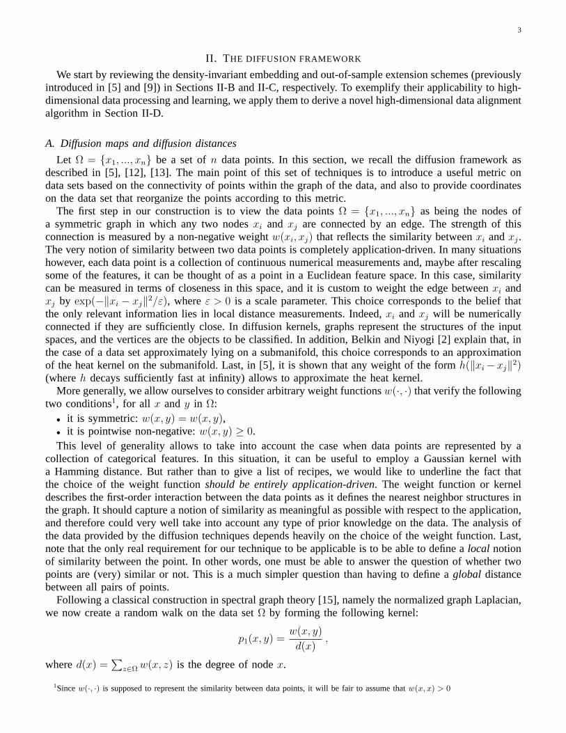
We can now build a classifier based on comparing a new trajectory to a collection of labeled trajectoriesin a training set. We randomly selected 20 instances of each digit to form a training set, the remaining20 being used as a testing set. In order to compare trajectories in the diffusion space, a metric is needed,and we chose to use the Hausdorff distance between two setsΓ1 andΓ2, defined as

dH(Γ1, Γ2) = max

maxx2∈Γ2

minx1∈Γ1

‖x1 − x2‖, maxx1∈Γ1

minx2∈Γ2

‖x1 − x2‖

.

Although this distance does not use the temporal information, it has the advantage of not being sensitive tothe choice of a parametrization or to the sampling density for either setΓ1 andΓ2. For a given trajectoryΓ from the testing set, our classifier is a nearest-neighbor classifier for this metric,i.e., the class ofΓ isdecided to be that of the nearest trajectory (fordH) in the training set. The performance of this classifieraveraged over 100 random trials is shown in Table I. In this case, the data set was embedded in 15dimensions.

“0” “1” “2” “3” “4” “5” “6” “7” “8” “9”zero 0.93 0 0 0.01 0 0 0.06 0 0 0one 0 1 0 0 0 0 0 0 0 0two 0.05 0 0.88 0.05 0.01 0 0.01 0 0 0

three 0.01 0 0.02 0.93 0 0 0.01 0.01 0.01 0.01four 0 0 0.01 0.01 0.97 0 0 0.01 0 0five 0 0 0 0.01 0 0.84 0.01 0.14 0 0.01six 0.04 0 0 0.01 0 0 0.92 0.02 0 0.01

seven 0.02 0 0 0.04 0 0.07 0.10 0.69 0.05 0.03eight 0 0.01 0 0 0 0.03 0.01 0.04 0.77 0.14nine 0 0 0 0.02 0 0 0 0.02 0.12 0.85

TABLE I

CLASSIFIER PERFORMANCE OVER100 RANDOM TRIALS. EACH ROW CORRESPONDS THE CLASSIFICATION DISTRIBUTION OF A GIVEN

DIGIT OVER THEN 10 CLASSES. THE DATA SET WAS EMBEDDED IN15 DIMENSIONS.

The classification error ranges from 0% to 31% with an average of 12.2%. The best classification rate isachieved for the word “one” which, in terms of visual information, stands far away from the other digits.In particular, typical sequences of “one” involve frames with a round open mouth, with no teeth visible(see first row of Figure 5). These frames essentially never appear for other digits. The worst classificationjob is for the word “seven” which seems to be highly confused with the words “five” and “six”. As shownon Figure 5, typical instances of these words appear to be similar in that the central frames involve anopen mouth with visible teeth. In the case of the “six” and “seven”, teeth from the lower jaws are visiblebecause of the “s” sound. Regarding the similarity between “five” and “seven”, the ”f” and ”v” soundstranslate into the lower lip touching the teeth of the upper jaw.

The accuracy that we obtain is comparable to former schemes [30], [41], while using significantlyless preprocessing. For instance, in [30], the lips images are hand picked and stabilized using an affinemotion model, while in [41] the contours of the lips are tracked by Active Contours. Our lips images areacquired by taping a continuous 5 minutes sequence and a simple cropping is performed to compensatefor translations. We note that the above comparison is qualitative rather than quantitative, as the differentschemes were applied to different datasets that are not publicly available.

B. Synchronization of head movement data

We now illustrate the concept of graph alignment as well as the algorithm presented in Section II-D.We recorded 3 movies of subjects wearing successively a yellow, red and black mask. Each subject wasasked to move their head in front of the camcorder. We then considered the three sets consisting of allframes of each movie. Let YELLOW, RED and BLACK denote these sets. Our goal was to synchronize

15

"FIVE"

"ONE"

"SEVEN"

"SIX"

Fig. 5. Typical frames for the words “one”, “five”, “six”, “seven”.

the movements of the different masks by aligning the 3 diffusion embeddings. The objective of thisexperiment was twofold

• We first wanted to illustrate the importance of having a coordinate system capturing the intrinsicgeometry of data sets. The intrinsic geometry is the basis of our alignment scheme: the key pointis that, as we will show, all three sets exhibit approximately the same intrinsic geometry, and thatthe diffusion coordinates parameterize this geometry. It is to be noted that working directly in imagespace would be highly inefficient since any picture of the red or black mask is at a large distance fromthe set of pictures of the yellow mask (this is a straight consequence of the high dimensionality of thedata). On the contrary, the diffusion coordinates will capture the intrinsic organization of each datasets, and therefore will provide a canonical representation of the sets that can be used for matchingthe data. Note also that our approach does not require any prior information on the type of data weare dealing with.

• The other point that we wished to illustrate is the importance of using the density-invariant diffusionmaps. As we will show, although the three sets have approximately the same intrinsic geometry (thedata points lie on the same 2D submanifold), the distribution of the points on this manifold are quitedifferent. Therefore, it is necessary to employ the density re-normalization technique described inSection II-B.

These two points constitute the main ingredients for a successful alignment of the sets.We now describe the experiment in more details. Each set of frames was regarded as a collection of

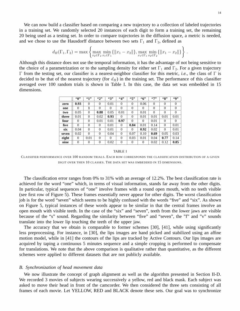
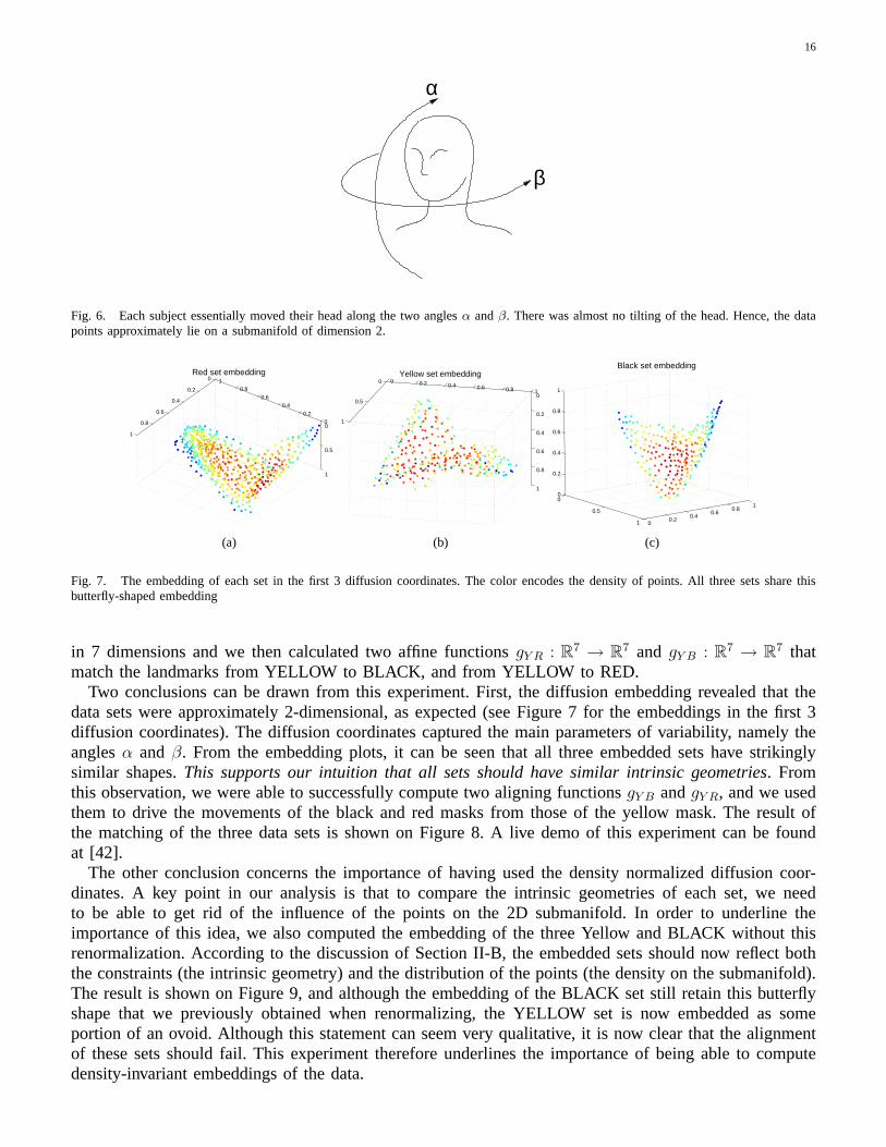
points inR10000, where the dimensionality coincides with the number of pixels per image. Following thelines of our algorithm, we formed a graph from each set with Gaussian weightsexp(−‖xi − xj‖2/ε).The quantity‖xi − xj‖ represents theL2 norm between imagesi and j, and here again, the scale waschosen so that each data point would be numerically connected to at least one other data point. We expecteach set to lie approximately on a manifold of dimension 2, as each subject essentially moved their headalong two anglesα andβ shown on Figure 6 and as the light conditions were kept the same during therecording. Therefore, each data sets is the expression of a highly constrained mechanical system, namelythe articulation between the neck and the head.

It is clear that the density of points on this manifold is essentially arbitrary and varies with each subjectand recording. Indeed, the density is essentially a function of the type of movement of each subject, theirspeed of execution, and also the type of mask that they were wearing. Since we were only interestedin the space of constraints, that is the geometry of the manifold, we renormalized the Gaussian weightsaccording to the algorithm described in Section II-B, and constructed a Markov chain that approximatesthe Laplace-Beltrami diffusion. Figure 7 shows the embedding in the first three eigenfunctions for eachdata set. They are extremely similar. We then defined 8 matching triplets of landmarks in each set. Thelandmarks were chosen to correspond to the main head positions. We computed the diffusion embedding

16

β

α

Fig. 6. Each subject essentially moved their head along the two anglesα andβ. There was almost no tilting of the head. Hence, the datapoints approximately lie on a submanifold of dimension 2.

0

0.2

0.4

0.6

0.8

1

0

0.2

0.4

0.6

0.8

1

0

0.5

1

Red set embedding

(a)

0

0.5

1

0 0.2 0.4 0.6 0.8 10

0.2

0.4

0.6

0.8

1

Yellow set embedding

(b)

0

0.5

1 00.2

0.40.6

0.81

0

0.2

0.4

0.6

0.8

1

Black set embedding

(c)

Fig. 7. The embedding of each set in the first 3 diffusion coordinates. The color encodes the density of points. All three sets share thisbutterfly-shaped embedding

in 7 dimensions and we then calculated two affine functionsgY R : R7 → R7 and gY B : R7 → R7 thatmatch the landmarks from YELLOW to BLACK, and from YELLOW to RED.

Two conclusions can be drawn from this experiment. First, the diffusion embedding revealed that thedata sets were approximately 2-dimensional, as expected (see Figure 7 for the embeddings in the first 3diffusion coordinates). The diffusion coordinates captured the main parameters of variability, namely theanglesα and β. From the embedding plots, it can be seen that all three embedded sets have strikinglysimilar shapes.This supports our intuition that all sets should have similar intrinsic geometries. Fromthis observation, we were able to successfully compute two aligning functionsgY B andgY R, and we usedthem to drive the movements of the black and red masks from those of the yellow mask. The result ofthe matching of the three data sets is shown on Figure 8. A live demo of this experiment can be foundat [42].

The other conclusion concerns the importance of having used the density normalized diffusion coor-dinates. A key point in our analysis is that to compare the intrinsic geometries of each set, we needto be able to get rid of the influence of the points on the 2D submanifold. In order to underline theimportance of this idea, we also computed the embedding of the three Yellow and BLACK without thisrenormalization. According to the discussion of Section II-B, the embedded sets should now reflect boththe constraints (the intrinsic geometry) and the distribution of the points (the density on the submanifold).The result is shown on Figure 9, and although the embedding of the BLACK set still retain this butterflyshape that we previously obtained when renormalizing, the YELLOW set is now embedded as someportion of an ovoid. Although this statement can seem very qualitative, it is now clear that the alignmentof these sets should fail. This experiment therefore underlines the importance of being able to computedensity-invariant embeddings of the data.

17

Fig. 8. The embedding of the YELLOW set in three diffusion coordinates and the various corresponding images after alignment of theRED and BLACK graphs to YELLOW.

−2

−1

0

1

2

−3−2−1012

−3

−2

−1

0

1

2

3

(a)

−4−2

02

4

−4−2

02

4

−2

−1

0

1

2

3

4

5

6

(b)

Fig. 9. The embeddings of the YELLOW (a) and BLACK (b) sets in three diffusion coordinates without the density renormalization. Theseembedded sets now have very different shapes, and their alignment is impossible.

IV. CONCLUSION AND FUTURE WORK

In this work we introduced diffusion techniques as a framework for data fusion and multi-cue datamatching by addressing several key issues. First, we underlined the importance of the Laplace-Beltraminormalization for data fusion by showing that it allows to merge data sets produced by the same sourcebut with different densities. In particular, the Laplace-Beltrami embedding provides a canonical, density-invariant embedding which is essential for data matching. Second, we suggested a new data fusion scheme,by extending spectral embeddings using the geometric harmonics framework. Finally, we presented a novelspectral graph alignment approach to data fusion.

Our scheme was successfully applied to lip-reading where we achieved high accuracy with minimalpreprocessing. We also demonstrated the alignment of high-dimensional visual data (“rotating heads”sequence).

In the work presented, we have focused on the situation when all sources are highly correlated. Inthe future we plan on extending our approach to multi-cue data analysis by integrating different signalsfrom weakly correlated sources into a unified representation. This should open the door to applicationsrelated to multi-sensor integration. Finally, we also are studying a spectral based approach to the analysis

18

of signals as dynamical random processes. Our current work did not utilize the temporal information ofthe video sequences. By constructing a dynamical Markov process model, we intend to improve the lipsreading accuracy.

V. ACKNOWLEDGMENTS

The authors would like to thank Steven Zucker for helpful discussions during the course of this workand Andreas Glaser for helping us out for the data collection. We also express our thanks to the refereesfor their constructive questions and comments.

APPENDIX IEXISTENCE AND UNIQUENESS OF THE STATIONARY DISTRIBUTION

The goal of this section is to show that if the graph is connected, then the stationary distributionφ0 isguaranteed to exist. The first step is to notice that the data set is finite, and therefore so is the state spaceof our Markov chain. Thus by a classical version of the Perron-Frobenius theorem, it suffices to provethat the chain is irreducible and aperiodic.

• The irreducibility is a mere consequence of the fact that the graph is connected. Indeed, letxi andxj be two data points, and letτ be the length of a path connectingxi and xj. Since the graph isconnected, we know thatτ < +∞. We conclude thatpτ (xi, xj) > 0, which implies that the chainirreducible.

• Concerning the aperiodicity, remember thatw(·, ·) represent the similarity between data points, sowe can assume that for all data pointxi, we havew(xi, xi) > 0. Consequently,p1(xi, xi) > 0, whichimplies that the chain is aperiodic.

Finally, we can conclude that our Markov chain has a unique stationary distributionφ0.

APPENDIX IIDIFFUSION DISTANCE AND EIGENFUNCTIONS

The random walk constructed from a graph via the normalized graph Laplacian procedure yields aMarkov matrix P with entriesp1(x, y). As it is well known [15], this matrix is in fact conjugate to asymmetric matrixA with entriesa(x, y), given by

a(x, y) =

√d(x)

d(y)p1(x, y) =

w(x, y)√d(x)d(y)

.

ThereforeA hasn eigenvaluesλ0, ..., λn−1 and orthonormal eigenvectorsv0, ..., vn−1. In particular,

a(x, y) =n−1∑

l=0

λlvl(x)vl(y) . (9)

This implies thatP has the samen eigenvalues. In addition, it hasn left eigenvectorsφ0, ..., φn−1 andnright eigenvectorsψ0, ..., ψn−1. Also, it can be checked that

φl(y) = vl(y)v0(y) andψl(x) = vl(x)/v0(x) . (10)

Furthermore, it can be verified thatv0(x) =√

d(x)/√∑

z d(z), and thereforeφ0(y) = d(y)/∑

z d(z) andψ0(x) = 1. In addition,

φ0(x)ψl(x) = φl(x) . (11)

It results from Equations 9 and 10 thatP t admits the following spectral decomposition:

pt(x, y) =n−1∑

l=0

λtlψl(x)φl(y) , (12)

19

together with the biorthogonality relation∑y∈Ω

φi(y)ψj(y) = δij , (13)

whereδij is Kronecker symbol. Combining this last identity with Equation 11, one obtains

∑y∈Ω

φi(y)φj(y)

φ0(y)= δij .

This means that the systemφl is orthonormal inL2(Ω, 1/φ0). Therefore, if one fixesx, Equation 12can interpreted as the decomposition of the functionpt(x, ·) over this system, where the coefficients ofdecomposition areλt

lψl(x).Now by definition,

Dt(x, z)2 =∑y∈Ω

(pt(x, y)− pt(z, y))2

φ0(y)= ‖pt(x, ·)− pt(z, ·)‖2

L2(Ω,1/φ0) .

Therefore,

Dt(x, y)2 =n−1∑

l=0

λ2tl (ψl(x)− ψl(z))2 .

REFERENCES

[1] S. Roweis and L. Saul, “Nonlinear dimensionality reduction by locally linear embedding,”Science, vol. 290, pp. 2323–2326, 2000.[2] M. Belkin and P. Niyogi, “Laplacian eigenmaps for dimensionality reduction and data representation,”Neural Computation, vol. 6,

no. 15, pp. 1373–1396, June 2003.[3] D. Donoho and C. Grimes, “Hessian eigenmaps: New locally linear embedding techniques for high-dimensional data,”Proceedings of

the National Academy of Sciences, vol. 100, no. 10, pp. 5591–5596, May 2003.[4] Z. Zhang and H. Zha, “Principal manifolds and nonlinear dimension reduction via local tangent space alignement,” Department of

computer science and engineering, Pennsylvania State University, Tech. Rep. CSE-02-019, 2002.[5] R. Coifman and S. Lafon, “Diffusion maps,”Applied and Computational Harmonic Analysis, 2006, to appear.[6] M. Belkin, P. Niyogi, and V. Sindhwani, “Manifold regularization: a geometric framework for learning from examples,” University of

Chicago, Tech. Rep. TR-2004-06, 2004.[7] C. Fowlkes, S. Belongie, F. Chung, and J. Malik, “Spectral grouping using the nyström method.”IEEE Transactions on Pattern Analysis

and Machine Intelligence, vol. 26, no. 2, pp. 214–225, 2004.[8] Y. Bengio, J.-F. Paiement, and P. Vincent, “Out-of-sample extensions for lle, isomap, mds, eigenmaps, and spectral clustering,” Université

de Montréal, Tech. Rep. 1238, 2003.[9] R. Coifman and S. Lafon, “Geometric harmonics: a novel tool for multiscale out-of-sample extension of empirical functions,”Applied

and Computational Harmonic Analysis, 2006, to appear.[10] R. Coifman, S. Lafon, A. Lee, M. Maggioni, B. Nadler, F. Warner, and S. W. Zucker, “Geometric diffusions as a tool for harmonic

analysis and structure definition of data: Diffusion maps,”Proceedings of the National Academy of Sciences, vol. 102, no. 21, pp.7426–7431, May 2005.

[11] R. Coifman, S. Lafon, A. Lee, M. Maggioni, B. Nadler, F. Warner, and S. Zucker, “Geometric diffusions as a tool for harmonicsanalysis and structure definition of data: Multiscale methods,”Proceedings of the National Academy of Sciences, vol. 102, no. 21, pp.7432–7437, May 2005.

[12] B. Nadler, S. Lafon, R. Coifman, and I. Kevrekidis, “Diffusion maps, spectral clustering and the reaction coordinates of dynamicalsystems,”Applied and Computational Harmonic Analysis, 2006, to appear.

[13] S. Lafon and A. B. Lee, “Diffusion maps and coarse-graining: A unified framework for dimensionality reduction, graph partitioningand data set parameterization,”IEEE Pattern Analysis and Machine Intelligence, 2006.

[14] R. I. Kondor and J. D. Lafferty, “Diffusion kernels on graphs and other discrete input spaces,” inICML ’02: Proceedings of theNineteenth International Conference on Machine Learning, 2002, pp. 315–322.

[15] F. Chung,Spectral graph theory. CBMS-AMS, May 1997, no. 92.[16] J. Shi and J. Malik, “Normalized cuts and image segmentation,”IEEE Tran PAMI, vol. 22, no. 8, pp. 888–905, 2000.[17] Y. Weiss, “Segmentation using eigenvectors: A unifying view.” inICCV, 1999, pp. 975–982.[18] M. Meila and J. Shi, “A random walk’s view of spectral segmentation,”AI and Statistics (AISTATS), 2001.[19] S. X. Yu and J. Shi, “Multiclass spectral clustering.” inProc. IEEE Int. Conf. Computer Vision, 2003, pp. 313–319.[20] M. Belkin and P. Niyogi, “Laplacian eigenmaps and spectral techniques for embedding and clustering.” inAdvances in Neural

Information Processing, 2001, pp. 585–591.[21] P. Diaconis and D. Stroock, “Geometric bounds for eigenvalues of markov chains,”The Annals of Applied Probability, vol. 1, no. 1,

pp. 36–61, 1991.

20

[22] M. Belkin and P. Niyogi, “Towards a theoretical foundation for laplacian-based manifold methods.” inCOLT, 2005, pp. 486–500.[23] W. Press, S. Teukolsky, W. Vetterling, and B. Flannery,Numerical Recipes in C. Cambridge University, 1988.[24] M. Gori, M. Maggini, and L. Sarti, “Exact and approximate graph matching using random walks.”IEEE Transactions on Pattern

Analysis and Machine Intelligence, vol. 27, no. 7, pp. 1100–1111, 2005.[25] J. Ham, D. Lee, and L. Saul, “Semisupervised alignment of manifolds,” inProceedings of the Tenth International Workshop on Artificial

Intelligence and Statistics, Jan 6-8, 2005, Savannah Hotel, Barbados, pp. 120–127.[26] X. Bai, H. Yu, and E. R. Hancock, “Graph matching using spectral embedding and alignment.” inICPR (3), 2004, pp. 398–401.[27] Y. Keselman, A. Shokoufandeh, M. F. Demirci, and S. J. Dickinson, “Many-to-many graph matching via metric embedding.” inCVPR

(1), 2003, pp. 850–857.[28] A. W. Fitzgibbon, “Robust registration of 2d and 3d point sets,” inProceedings of the British Machine Vision Conference, 2001, pp.

662–670.[29] H. J. Wolfson and I. Rigoutsos, “Geometric hashing: An overview,”IEEE Comput. Sci. Eng., vol. 4, no. 4, pp. 10–21, 1997.[30] M. Aharon and R. Kimmel, “Representation analysis and synthesis of lip images using dimensionality reduction,”Accepted to the

International Journal of Computer Vision.[31] B. Christoph, C. Michele, and S. Malcolm, “Video rewrite: driving visual speech with audio,” inSIGGRAPH ’97: Proceedings of

the 24th annual conference on Computer graphics and interactive techniques. New York, NY, USA: ACM Press/Addison-WesleyPublishing Co., 1997, pp. 353–360.

[32] E. Cosatto and H. P. Graf, “Photo-realistic talking-heads from image samples.”IEEE Transactions on Multimedia, vol. 2, no. 3, pp.152–163, 2000.

[33] C. Bregler, S. Manke, and H. Hild, “Improving connected letter recognition by lipreading,” inProc. IEEE Int. Conf. Acoust., Speechand Signal Processing, 1993.

[34] N. Dettmer and M. Shah, “Visually recognizing speech using eigensequences,”Computational Imaging and Vision, pp. 345–371, 1997.[35] I. Matthews, T. Cootes, A. Bangham, S. Cox, and R. Harvey, “Extraction of visual features for lipreading.”IEEE Transactions on

Pattern Analysis and Machine Intelligence, vol. 24, no. 2, pp. 198–213, 2002.[36] A. V. Nefian, L. H. Liang, X. X. Liu, X. Pi, and K. Murphy, “Dynamic bayesian networks for audio-visual speech recognition,”Journal

of Applied Signal Processing,, vol. 2002, no. 11„ pp. 1274–1288, 2002.[37] J. Luettin, N. A. Thacker, and S. W. Beet, “Active shape models for visual speech feature extraction,” inSpeechreading by Humans

and Machines, ser. NATO ASI Series, Series F: Computer and Systems Sciences, D. G. Storck and M. E. H. (editors), Eds. Berlin:Springer Verlag, 1996, vol. 150, pp. 383–390.

[38] J. Luettin and N. A. Thacker, “Speechreading using probabilistic models,”Computer Vision and Image Understanding, vol. 65, no. 02,pp. 163–178, 1997.

[39] Y.-L. Tian, T. Kanade, and J. Cohn, “Robust lip tracking by combining shape, color and motion,” inProceedings of the 4th AsianConference on Computer Vision (ACCV’00), January 2000.

[40] I. Borg and P. Groenen,Modern Multidimensional Scaling - Theory and Applications. Springer-Verlag New York Inc., 1997.[41] C. Bregler, S.Omohundro, M.Covell, M.Slaney, S.Ahmad, D.A.Forsyth, and J.A.Feldman, “Probabilistic models of verbal and body

gestures,” inComputer Vision in Man-Machine Interfaces, R. Cipolla and A. eds, Eds. Cambridge University Press, 1998.[42] S. Lafon, “Demo of the mask alignment,” 2005. [Online]. Available: http://www.math.yale.edu/∼sl349/demos_data/demos.htm.

Stéphane Lafon is a Software Engineer at Google. He received his B.Sc. degree in Computer Science from EcolePolytechnique and his M.Sc. in Mathematics and Artificial Intelligence from Ecole Normale Supérieure de Cachan inFrance. He obtained his Ph.D. in Applied Mathematics at Yale University in 2004 and he was a research associate inthe Mathematics Department during 2004-2005. He is currently with Google where his work focuses on the design,analysis and implementation of machine learning algorithms. His research interests are in data mining, machine learningand information retrieval.

Yosi Keller received the B.Sc. degree in electrical engineering in 1994 from The Technion-Israel Institute of Tech-nology, Haifa. He received the M.Sc and Ph.D degree in electrical engineering from Tel-Aviv University, Tel-Aviv,in 1998 and 2003, respectively. From 1994 to 1998, he was an R&D Officer in the Israeli Intelligence Force. Heis a visiting Assistant Professor with the Department of Mathematics, Yale University. His research interests includemotion estimation and statistical pattern analysis.

21

Ronald R. Coifman is the Phillips Professor of Mathematics at Yale University. His research interests include: nonlinearFourier analysis, wavelet theory, singular integrals, numerical analysis and scattering theory, and new mathematicaltools for efficient computation and transcriptions of physical data, with applications to numerical analysis, featureextraction recognition and denoising. Professor Coifman, who earned his Ph.D. at the University of Geneva in 1965,is a member of the National Academy of Sciences and the American Academy of Arts and Sciences. He received theDARPA Sustained Excellence Award in 1996, the 1999 Pioneer Award from the International Society for Industrialand Applied Mathematics. He is a recipient of National Medal of Science.