
1 Combinatorial Dominance Analysis The Knapsack Problem Keywords: Combinatorial Dominance (CD)...
72
1 Combinatorial Dominance Analysis The Knapsack Problem Keywords: Combinatorial Dominance (CD) Domination number/ratio (domn, domr) Knapsack (KP) Incremental Insertion (II) Local Exchange (LE) PTAS Optimal Head - Greedy Tail (GRT) Presented by: Yochai Twitto
-
date post
21-Dec-2015 -
Category
Documents
-
view
225 -
download
2
Transcript of 1 Combinatorial Dominance Analysis The Knapsack Problem Keywords: Combinatorial Dominance (CD)...
1
Combinatorial Dominance Analysis
The Knapsack Problem
Keywords:Combinatorial Dominance (CD)Domination number/ratio (domn, domr)
Knapsack (KP)
Incremental Insertion (II)Local Exchange (LE)PTAS Optimal Head - Greedy Tail (GRT)
Presented by:
Yochai Twitto

2
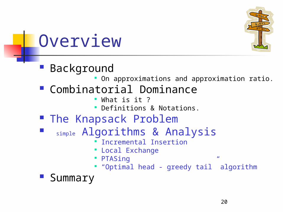
Overview Background
On approximations and approximation ratio. Combinatorial Dominance
What is it ? Definitions & Notations.
The Knapsack Problem simple Algorithms & Analysis
Incremental Insertion Local Exchange PTASing “Optimal head - greedy tail” algorithm
Summary
3
Overview Background
On approximations and approximation ratio. Combinatorial Dominance
What is it ? Definitions & Notations.
The Knapsack Problem simple Algorithms & Analysis
Incremental Insertion Local Exchange PTASing “Optimal head - greedy tail” algorithm
Summary

4
Background NP complexity class.
AA and quality of approximations.
The classical approximation ratio analysis.
5
NP
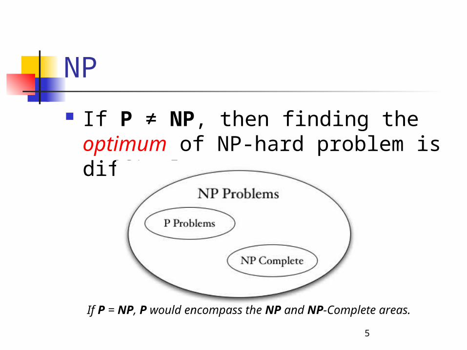
If P ≠ NP, then finding the optimum of NP-hard problem is difficult.
If P = NP, P would encompass the NP and NP-Complete areas.
6
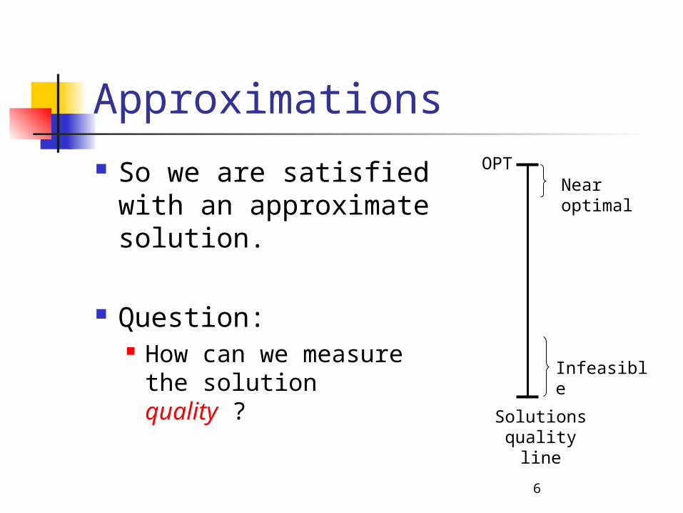
Approximations
So we are satisfied with an approximate solution.
Question: How can we measure
the solution quality ?Solutions
quality line
OPT
Infeasible
Near optimal
7
Solution Quality
Most of the time, naturally derived from the problem definition.
If not, it should be given as external information.
8
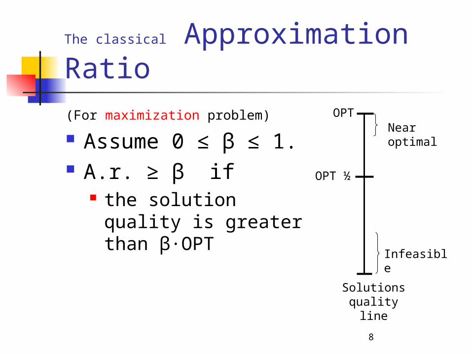
The classical Approximation Ratio(For maximization problem)
Assume 0 ≤ β ≤ 1. A.r. ≥ β if
the solution quality is greater than β·OPT
Solutions quality line
OPT
Infeasible
Near optimal
½OPT
9
Overview Background
On approximations and approximation ratio. Combinatorial Dominance
What is it ? Definitions & Notations.
The Knapsack Problem simple Algorithms & Analysis
Incremental Insertion Local Exchange PTASing “Optimal head - greedy tail” algorithm
Summary
10
Combinatorial Dominance
What is a “combinatorial dominance guarantee” ?
Why do we need such guarantees ?
Definitions and notations.

11
What is a
“combinatorial dominance guarantee” ?
A letter of reference: “She is half as good as I am, but I am the best
in the world…” “she finished first in my class of 75 students…”
The former is akin to an approximation ratio.
The latter to combinatorial dominance guarantee.
12
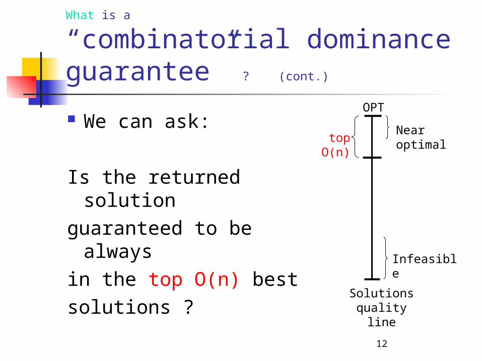
What is a
“combinatorial dominance guarantee” ? (cont.)
We can ask:
Is the returned solution
guaranteed to be always
in the top O(n) bestsolutions ?
Solutions quality line
OPT
Infeasible
Near optimaltop
O(n)
13
Why do we need that ?
Assume an problem for which all solutions are at least a half as good as optimal solution.
Then, 2-factor approximating the problem is meaningless.
14
Corollary
The approximation ratio analysis gives us only a partial insight of the performance of the algorithm.
Dominance analysis makes the picture fuller.

15
Definitions & Notations
Domination number: domn
Domination ratio: domr

16
Domination Number: domn Let P be a CO problem. Let A be an approximation for P .
For an instance I of P, the domination number domn(I, A) of A on I is the number of feasible solutions of I that are not better than the solution found by A.
17
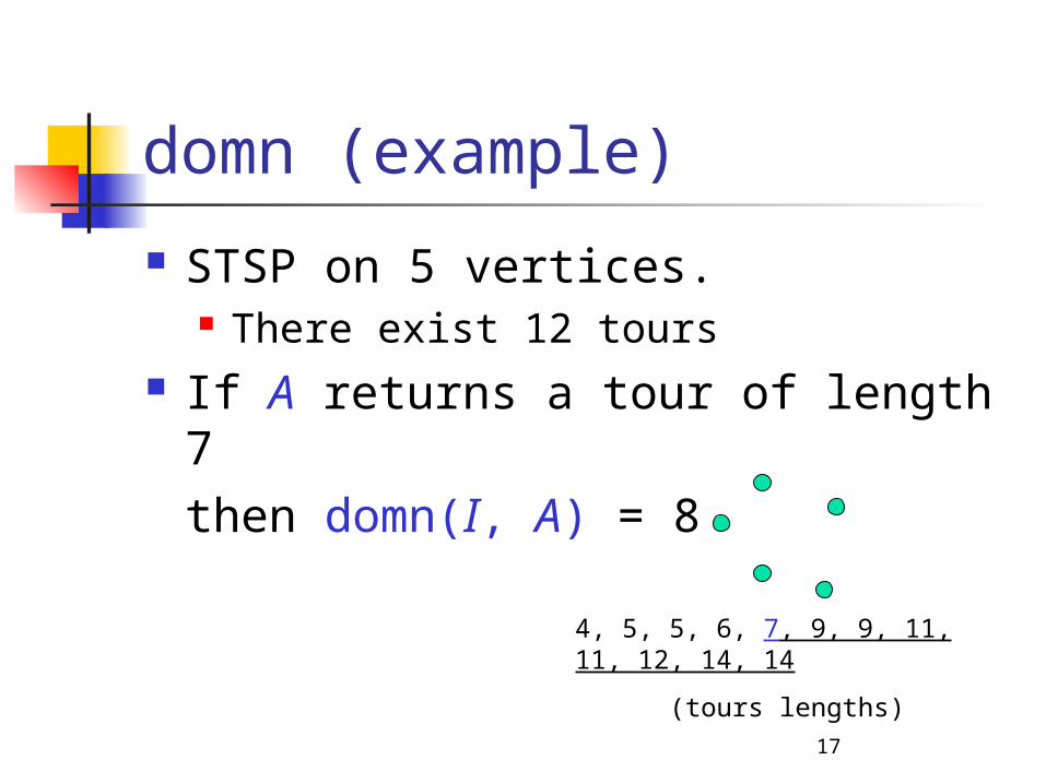
domn (example)
STSP on 5 vertices. There exist 12 tours
If A returns a tour of length 7 then domn(I, A) = 8
4, 5, 5, 6, 7, 9, 9, 11, 11, 12, 14, 14
(tours lengths)
18
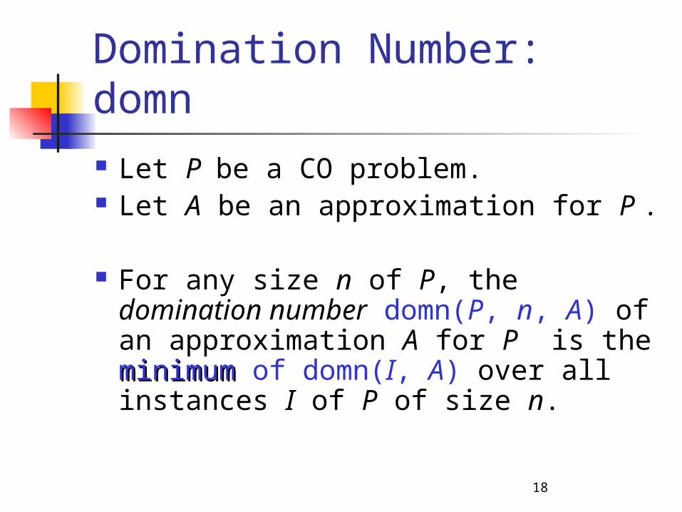
Domination Number: domn Let P be a CO problem. Let A be an approximation for P .
For any size n of P, the domination number domn(P, n, A) of an approximation A for P is the minimumminimum of domn(I, A) over all instances I of P of size n.
19
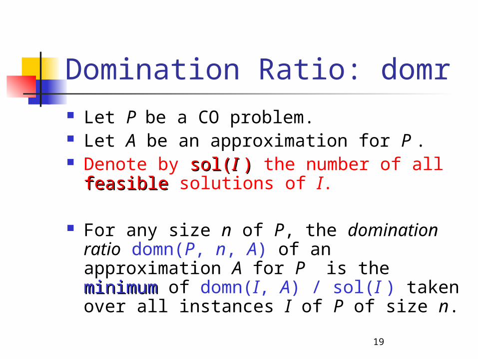
Domination Ratio: domr Let P be a CO problem. Let A be an approximation for P . Denote by sol(sol(I I )) the number of all
feasiblefeasible solutions of I.
For any size n of P, the domination ratio domn(P, n, A) of an approximation A for P is the minimumminimum of domn(I, A) / sol(I ) taken over all instances I of P of size n.
20
Overview Background
On approximations and approximation ratio. Combinatorial Dominance
What is it ? Definitions & Notations.
The Knapsack Problem simple Algorithms & Analysis
Incremental Insertion Local Exchange PTASing “Optimal head - greedy tail” algorithm
Summary
21
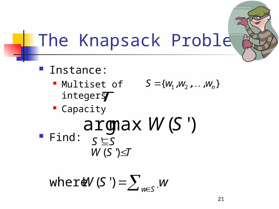
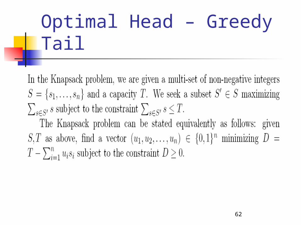
The Knapsack Problem Instance:
Multiset of integers
Capacity
Find:
},,,{ 21 nwwwS T
)'(maxarg
)'('
SW
TSWSS
')'( where
SwwSW
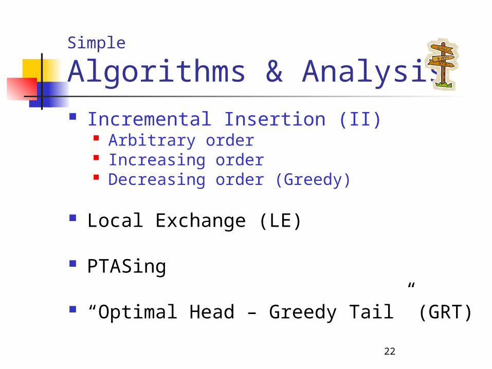
22
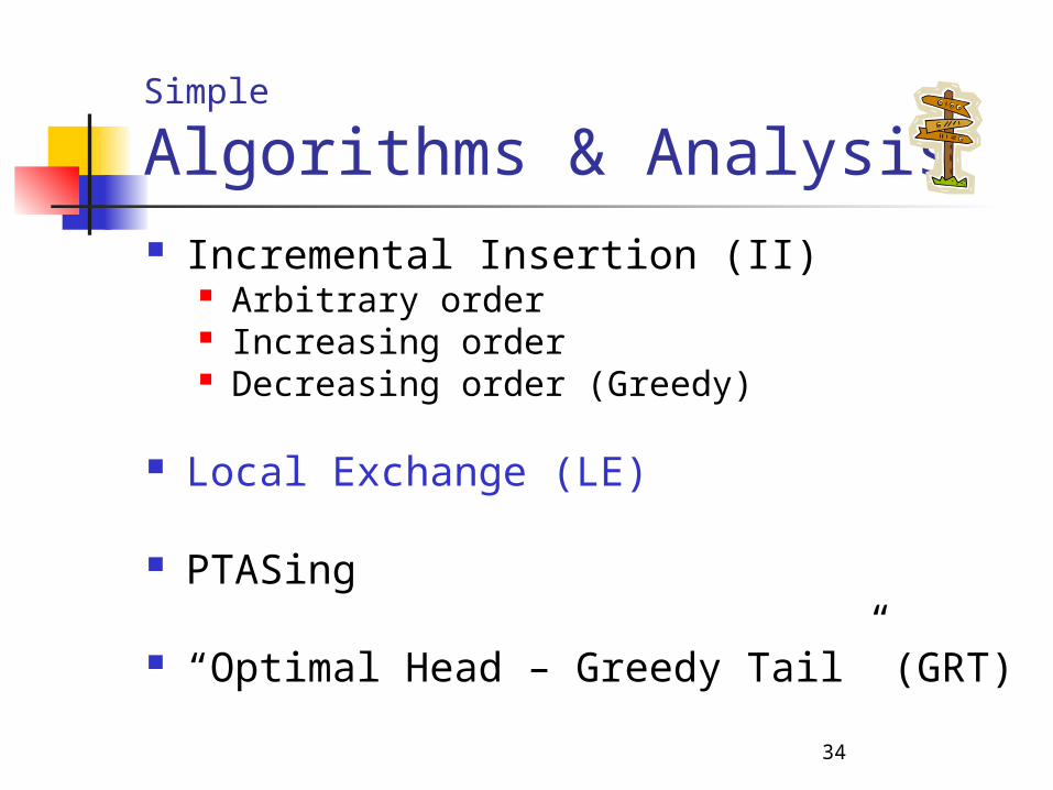
Simple
Algorithms & Analysis Incremental Insertion (II)
Arbitrary order Increasing order Decreasing order (Greedy)
Local Exchange (LE)
PTASing
“Optimal Head – Greedy Tail” (GRT)

23
II – Arbitrary Order
Go over the elements (arbitrary order)
Insert an element if the capacity not exceeded
Theorem: 12),,domn( 1 nnIIKP
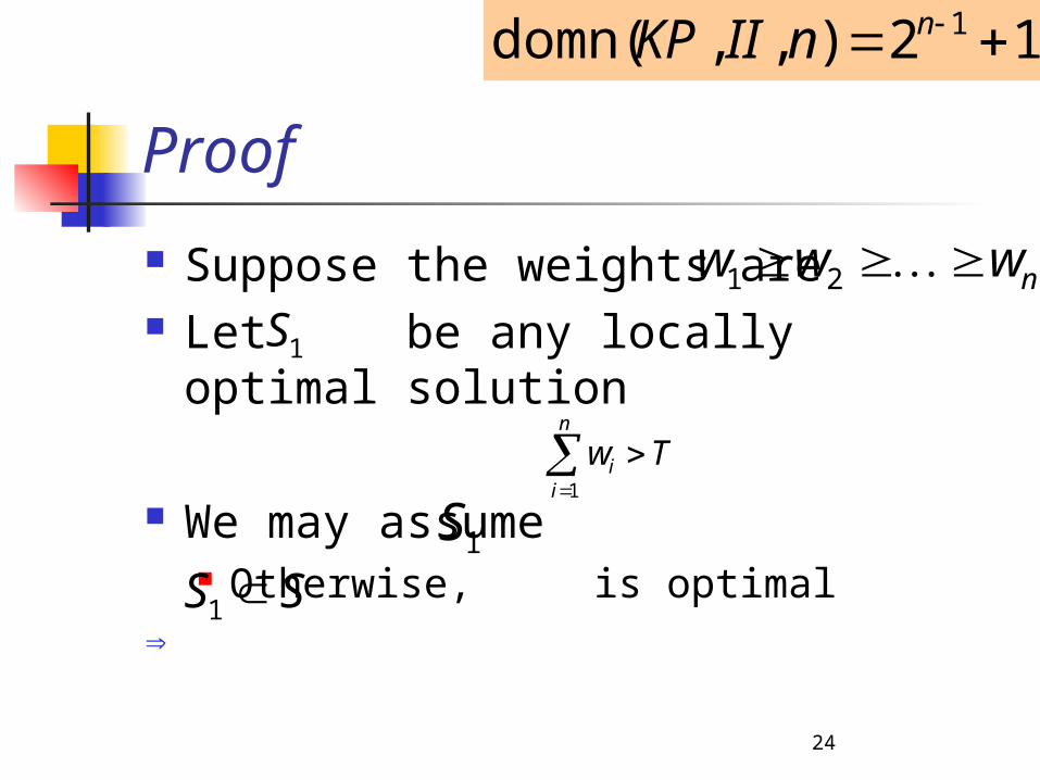
24
Proof
Suppose the weights are Let be any locally optimal
solution
We may assume Otherwise, is optimal
12),,domn( 1 nnIIKP
nwww 21
1S
Twn
ii
1
1SSS 1

25
Proof (cont.)
Let be the largest index of a weight not belonging to
Since is locally optimal
k
1S
kwTSW )( 1
1S
12),,domn( 1 nnIIKP
9 8 7 6 3 2 :
12 11 10 5 4 1:
1
1
CS
S
26
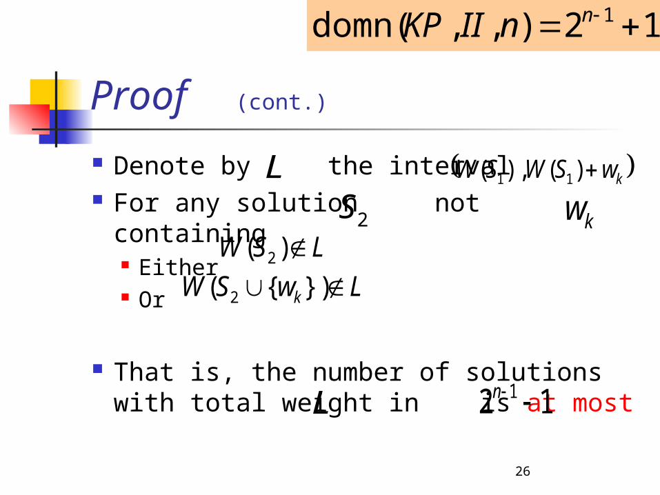
Proof (cont.)
Denote by the interval For any solution not containing
Either Or
That is, the number of solutions with total weight in is at most
12),,domn( 1 nnIIKP
L kwSWSW )(),( 11
2S kwLSW )( 2
LwSW k }){( 2
12 1 nL

27
Proof (cont.)
Solutions of weight at leastare infeasible.
Solution weighted not more than are not better than
12),,domn( 1 nnIIKP
kwSW )( 1
)( 1SW
1S
12),,domn( 1 nnIIKP
28
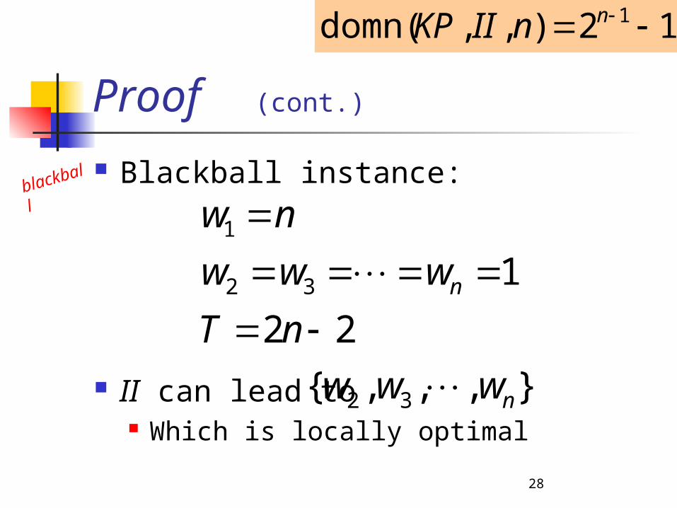
Proof (cont.)
Blackball instance:
II can lead to Which is locally optimal
12),,domn( 1 nnIIKP
22
132
1
nT
www
nw
n
},,,{ 32 nwww
blackba
ll
29
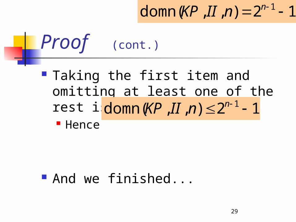
Proof (cont.)
Taking the first item and omitting at least one of the rest is better.
Hence
And we finished...
12),,domn( 1 nnIIKP
12),,domn( 1 nnIIKP

30
II – Increasing Order
No Gain!
That was our blackball… In the previous proof.
31
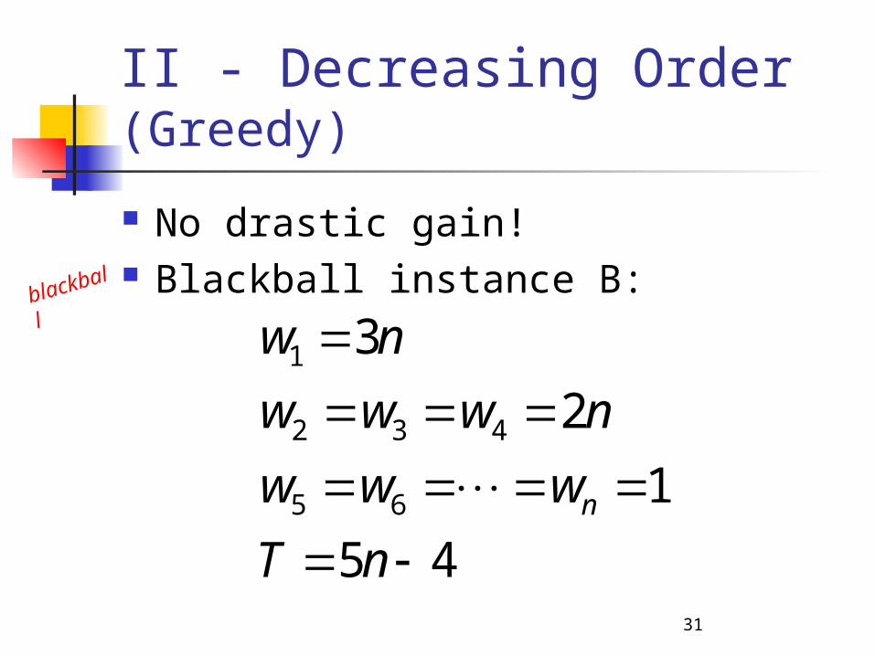
II - Decreasing Order (Greedy)
No drastic gain! Blackball instance B:blackba
ll
45
1
2
3
65
432
1
nT
www
nwww
nw
n

32
II - Decreasing Order (Greedy)
Greedy(B) Weight:
Any solution taking Exactly two elements from Any of the last elements
is better!
},,,,{ 651 nwwww 44 n
432 ,, www4n
33
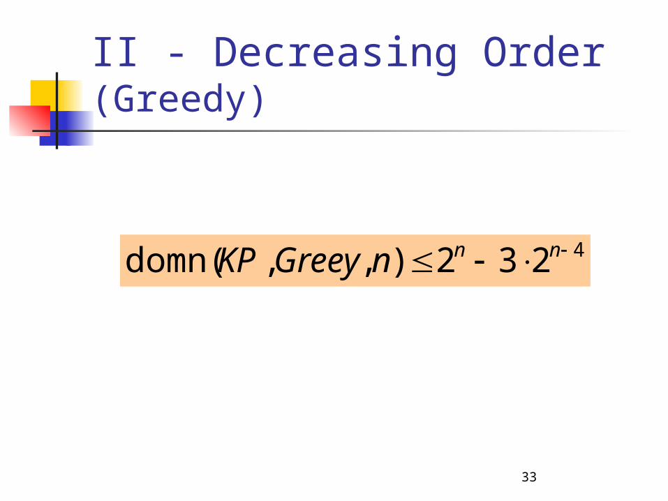
II - Decreasing Order (Greedy)
4232),,domn( nnnGreeyKP
34
Simple
Algorithms & Analysis Incremental Insertion (II)
Arbitrary order Increasing order Decreasing order (Greedy)
Local Exchange (LE)
PTASing
“Optimal Head – Greedy Tail” (GRT)
35
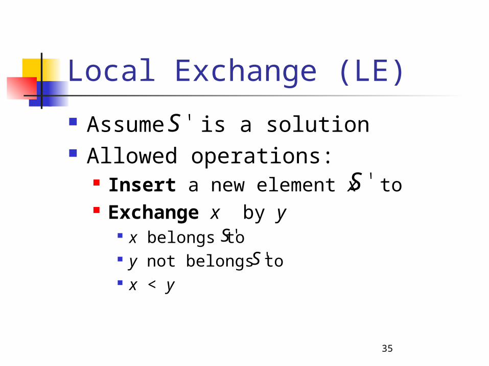
Local Exchange (LE)
Assume is a solution Allowed operations:
Insert a new element x to Exchange x by y
x belongs to y not belongs to x < y
'S
'S
'S'S
36
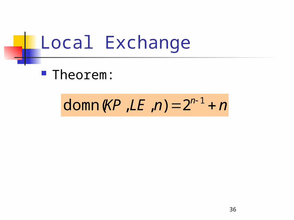
Local Exchange
Theorem:
nnLEKP n 12),,domn(

37
Proof
Suppose the weights are Let be any locally optimal
solution
We may assume Otherwise, is optimal
nwww 21
1S
Twn
ii
1
1SSS 1
nnLEKP n 12),,domn(
38
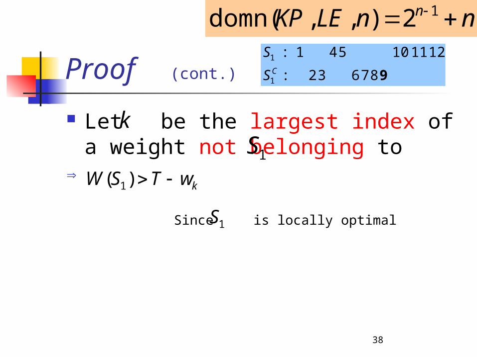
Proof (cont.)
Let be the largest index of a weight not belonging to
Since is locally optimal
k
1S
kwTSW )( 1
1S
nnLEKP n 12),,domn(
9 8 7 6 3 2 :
12 11 10 5 4 1:
1
1
CS
S

39
Proof (cont.)
Denote by the interval For any solution not containing
Either Or
That is, the number of solutions with total weight in is at most
And there are at least outside
L kwSWSW )(),( 11
kwLSW )( 2
LwSW k }){( 2
12 1 n
nnLEKP n 12),,domn(
9 8 7 6 3 2 :
12 11 10 5 4 1:
1
1
CS
S
12 1 nL
2S
40
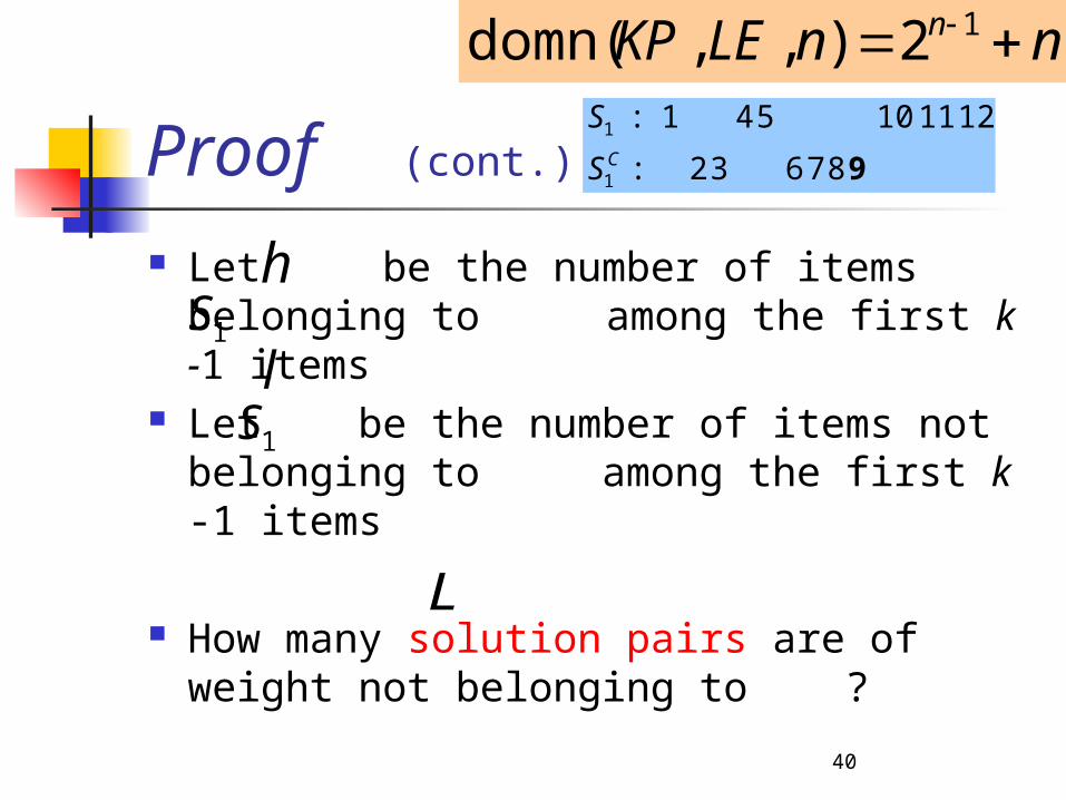
Proof (cont.)
Let be the number of items belonging to among the first k -1 items
Let be the number of items not belonging to among the first k -1 items
How many solution pairs are of weight not belonging to ?
nnLEKP n 12),,domn(
9 8 7 6 3 2 :
12 11 10 5 4 1:
1
1
CS
S
h1Sl1S
L
41
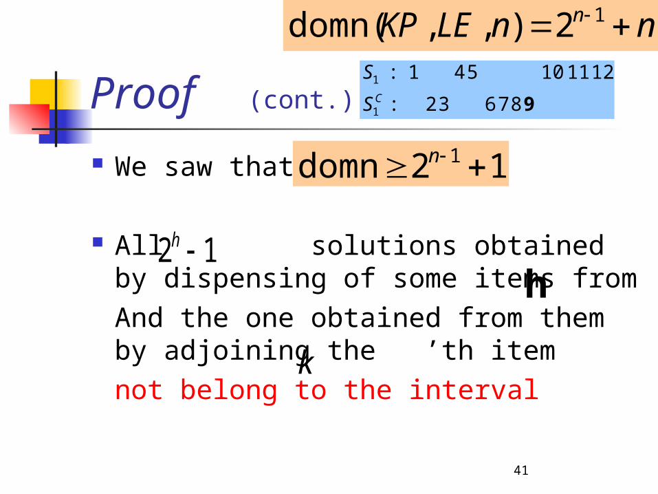
Proof (cont.)
We saw that
All solutions obtained by dispensing of some items fromAnd the one obtained from them by adjoining the ’th item not belong to the interval
12domn 1 n
12 h
nnLEKP n 12),,domn(
9 8 7 6 3 2 :
12 11 10 5 4 1:
1
1
CS
S
h
k
42
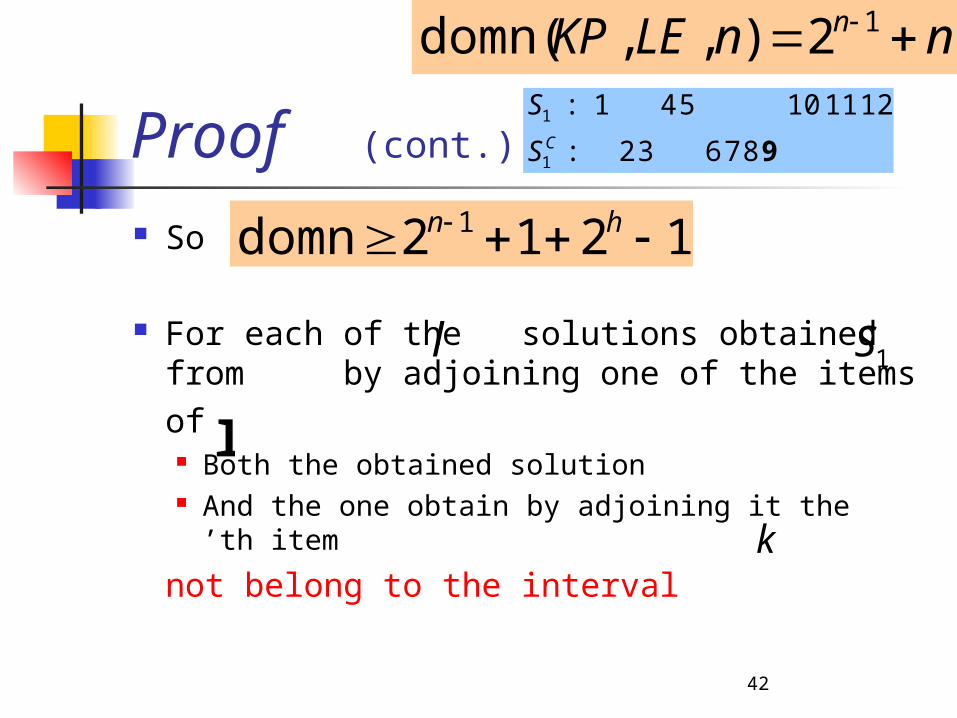
Proof (cont.)
So
For each of the solutions obtained from by adjoining one of the itemsof
Both the obtained solution And the one obtain by adjoining it the ’th
item
not belong to the interval
1212domn 1 hn
nnLEKP n 12),,domn(
9 8 7 6 3 2 :
12 11 10 5 4 1:
1
1
CS
S
l 1S
l
k
43
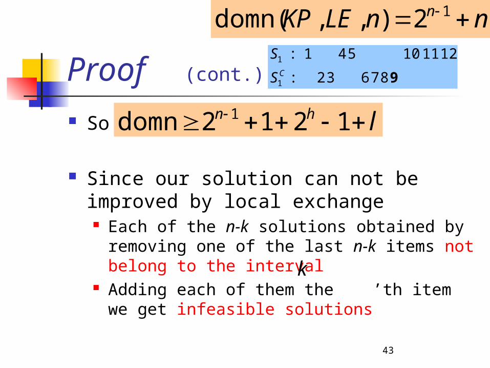
Proof (cont.)
So
Since our solution can not be improved by local exchange
Each of the n-k solutions obtained by removing one of the last n-k items not belong to the interval
Adding each of them the ’th item we get infeasible solutions
lhn 1212domn 1
nnLEKP n 12),,domn(
9 8 7 6 3 2 :
12 11 10 5 4 1:
1
1
CS
S
k
44
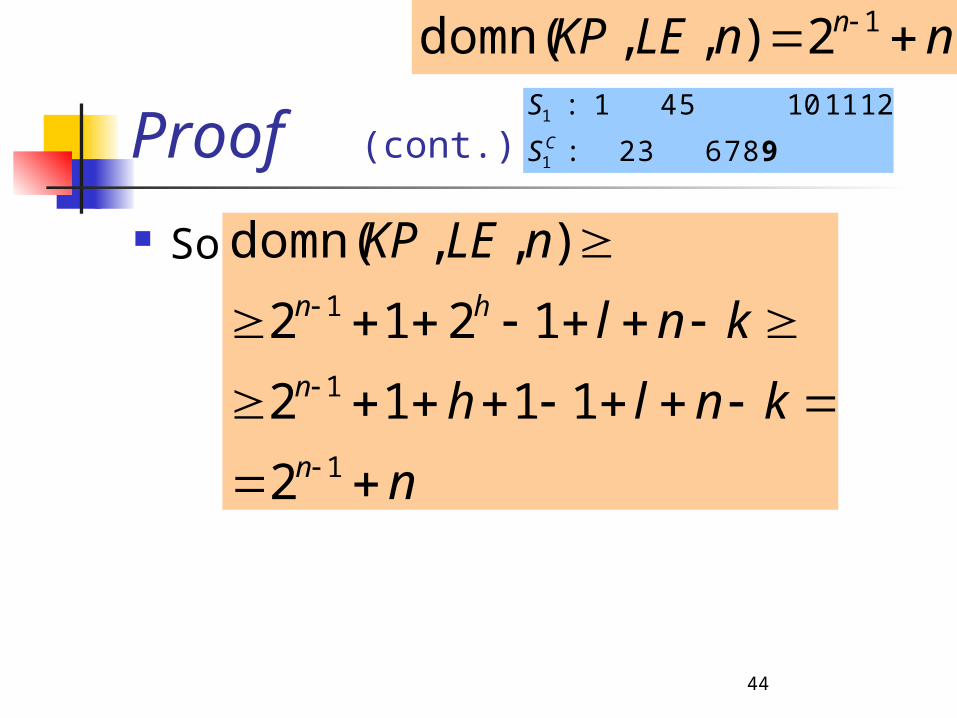
Proof (cont.)
So
n
knlh
knl
nLEKP
n
n
hn
1
1
1
2
1112
1212
),,domn(
nnLEKP n 12),,domn(
9 8 7 6 3 2 :
12 11 10 5 4 1:
1
1
CS
S

45
Proof (cont.)
Blackball instance:
LE can lead to Which is locally optimal
12),,domn( 1 nnIIKP
32
132
1
nT
www
nw
n
},,,{ 32 nwww
blackba
ll
nnLEKP n 12),,domn(

46
Proof (cont.)
Taking the first item and omitting at least two of the rest is better.
Hence:
And we finished...
12),,domn( 1 nnIIKP nnLEKP n 12),,domn(
n
nnLEKPn
nn
1
1
2
)]1(12[2),,domn(
b(n)
47
Simple
Algorithms & Analysis Incremental Insertion (II)
Arbitrary order Increasing order Decreasing order (Greedy)
Local Exchange (LE)
PTASing
“Optimal Head – Greedy Tail” (GRT)
48
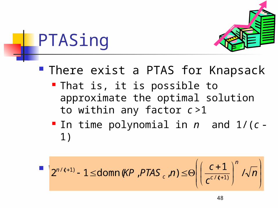
PTASing
There exist a PTAS for Knapsack That is, it is possible to approximate
the optimal solution to within any factor c >1
In time polynomial in n and 1/(c -1)
We’ll see
n
c
cnPTASKP
n
ccccn /
1),,domn(12
)1/()1/(
49
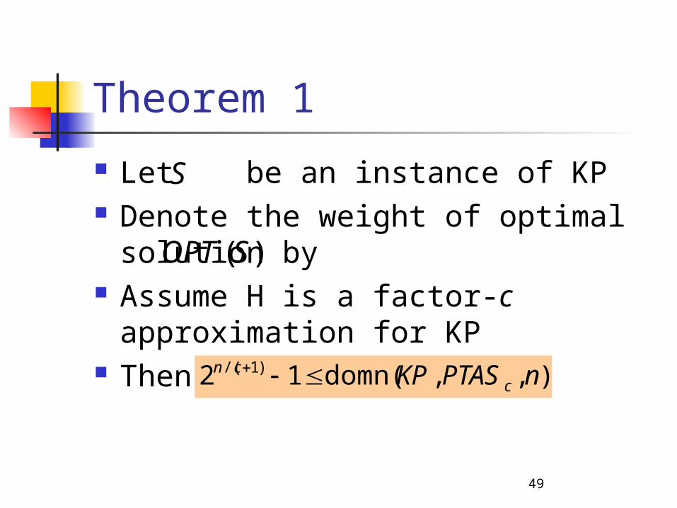
Theorem 1
Let be an instance of KP Denote the weight of optimal
solution by Assume H is a factor-c
approximation for KP Then ),,domn(12 )1/( nPTASKP c
cn
S
)(SOPT
50
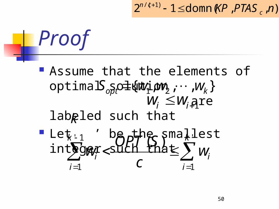
Proof Assume that the elements of
optimal solution are labeled such that
Let ’ be the smallest integer such that
),,domn(12 )1/( nPTASKP ccn
'
1
1'
1
)( k
ii
k
ii w
c
SOPTw
},,,{ 21 kopt wwwS 1 ii ww
k
51
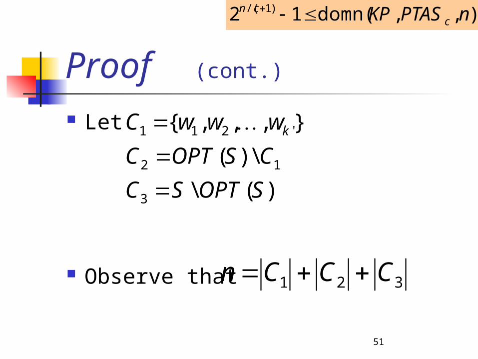
Proof (cont.)
Let
Observe that
),,domn(12 )1/( nPTASKP ccn
)(\
\)(
},,,{
3
12
'211
SOPTSC
CSOPTC
wwwC k
321 CCCn

52
Proof (cont.)
Also note that Since
The weight of every element of is not more than the weight of any element of
is a c -approximated solution to
),,domn(12 )1/( nPTASKP ccn
12 )1( CcC
1C
1C2C
21 CCSopt
53
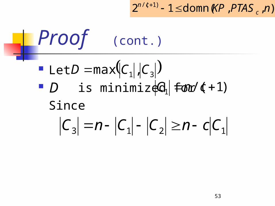
Proof (cont.)
Let is minimized for
Since
),,domn(12 )1/( nPTASKP ccn
31 ,max CCD )1/(1 cnC
1213 CcnCCnC
D
54
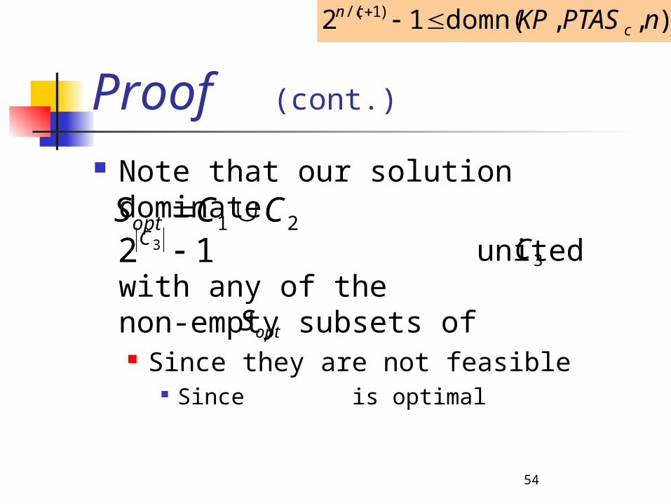
Proof (cont.)
Note that our solution dominate united with any of the
non-empty subsets of Since they are not feasible
Since is optimal
),,domn(12 )1/( nPTASKP ccn
21 CCSopt 12 3 C
3C
optS
55
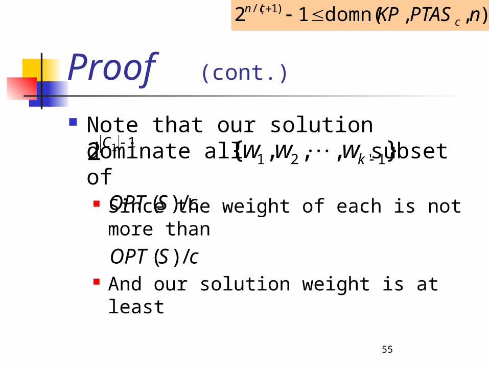
Proof (cont.)
Note that our solution dominate all subset of
Since the weight of each is not more than
And our solution weight is at least
),,domn(12 )1/( nPTASKP ccn
112 C },,,{ 1'21 kwww
cSOPT /)(
cSOPT /)(

56
Proof (cont.)
Summing both terms, the number of solution dominated is
Minimizing the left-hand term we get the result.
),,domn(12 )1/( nPTASKP ccn
113 212 CC
57
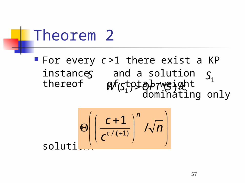
Theorem 2 For every c >1 there exist a KP
instance and a solution thereof of total weight dominating only
solution.
nc
cn
cc/
1)1/(
S1S
cSOPTSW /)()( 1
58
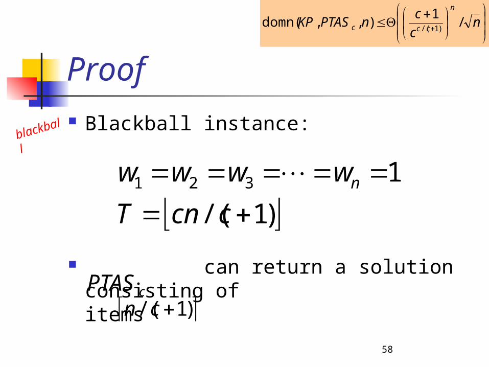
Proof Blackball instance:
can return a solution consisting of items
)1/(
1321
ccnT
wwww nblackba
ll
nc
cnPTASKP
n
ccc /1
),,domn()1/(
cPTAS )1/( cn
59
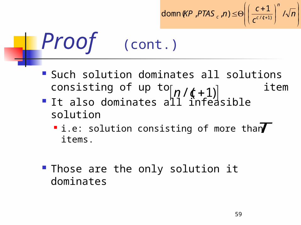
Proof (cont.)
Such solution dominates all solutions consisting of up to item
It also dominates all infeasible solution i.e: solution consisting of more than items.
Those are the only solution it dominates
nc
cnPTASKP
n
ccc /1
),,domn()1/(
)1/( cn
T
60
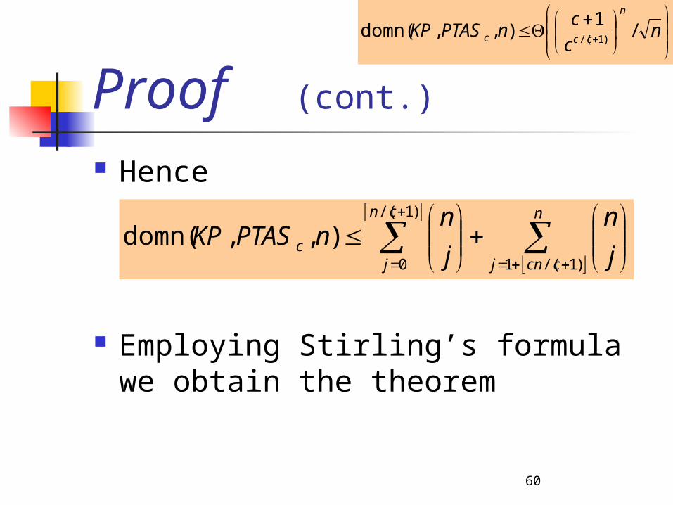
Proof (cont.)
Hence
Employing Stirling’s formula we obtain the theorem
nc
cnPTASKP
n
ccc /1
),,domn()1/(
n
ccnj
cn
jc j
n
j
nnPTASKP
)1/(1
)1/(
0
),,domn(
61
Simple
Algorithms & Analysis Incremental Insertion (II)
Arbitrary order Increasing order Decreasing order (Greedy)
Local Exchange (LE)
PTASing
“Optimal Head – Greedy Tail” (GRT)
62
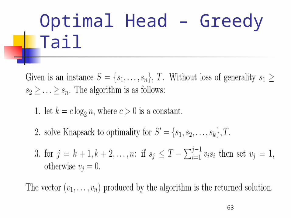
Optimal Head – Greedy Tail
63
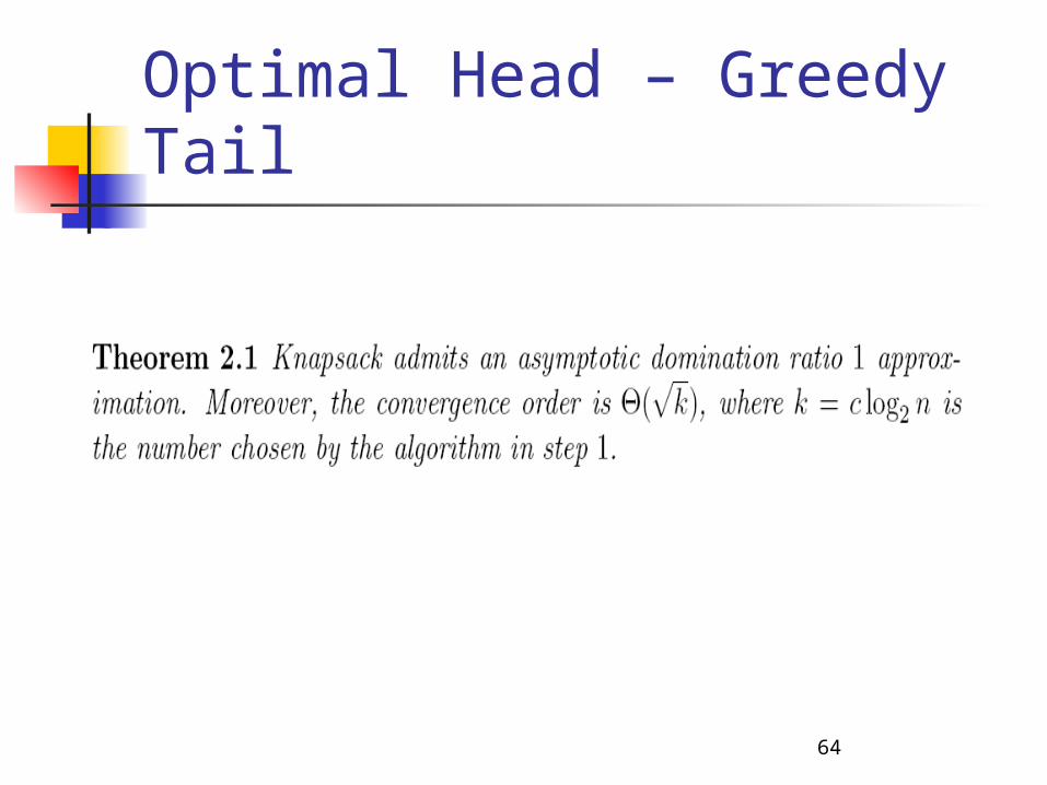
Optimal Head – Greedy Tail
64
Optimal Head – Greedy Tail
65
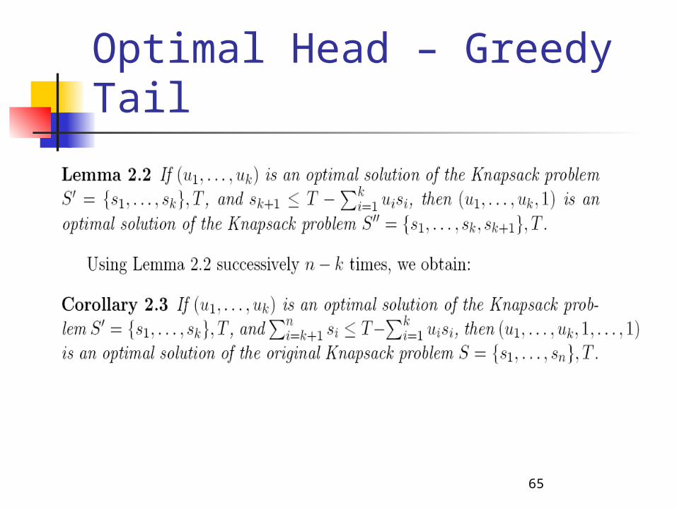
Optimal Head – Greedy Tail
66
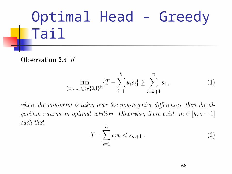
Optimal Head – Greedy Tail

67
Optimal Head – Greedy Tail

68
Optimal Head – Greedy Tail
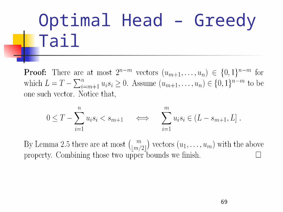
69
Optimal Head – Greedy Tail

70
Optimal Head – Greedy Tail

71
Summary
12),,domn( 1 nnIIKP
4232),,domn( nnnGreeyKP
nnLEKP n 12),,domn(
n
c
cnPTASKP
n
ccccn /
1),,domn(12
)1/()1/(
nnGRTKP n log/112),,domn(
72
Combinatorial Dominance Analysis
The Knapsack Problem


