1 Clipping and Hidden Surfaces CS-184: Computer Graphics Prof. James O’Brien.
45
1 Clipping and Hidden Surfaces CS-184: Computer Graphics Prof. James O’Brien
-
date post
21-Dec-2015 -
Category
Documents
-
view
219 -
download
0
Transcript of 1 Clipping and Hidden Surfaces CS-184: Computer Graphics Prof. James O’Brien.

1
Clipping andHidden Surfaces
CS-184: Computer Graphics
Prof. James O’Brien

2
Clipping
• Don’t want to draw stuff that is not in screen area– Waste of time
– Bogus memory access
– Looks ugly
• Clipping removes unwanted stuff• Can also clip for other reasons
– Cut away views
3
Basic Line Clipping

4
Cohen-Sutherland Line Clip
• Clip line against each edge of clip region in turn– If both endpoints outside, discard line and stop
– If both endpoints in, continue to next edge (or finish)
– If one in, one out, chop line at crossing pt and continue
• Works in both 2D and 3D for convex clipping regions

5
Cohen-Sutherland Line Clip
1 2
3
4
1 2
3
4
1 2
3
4
1 2
3
4
6
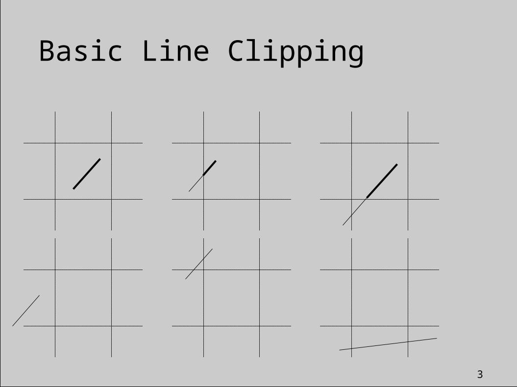
Cohen-Sutherland Line Clip
• Trivial reject and accept (speed things up…)
Trivial Keep NOT Trivial RejectTrivial Reject
7
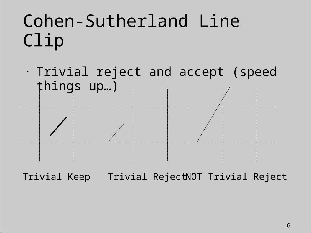
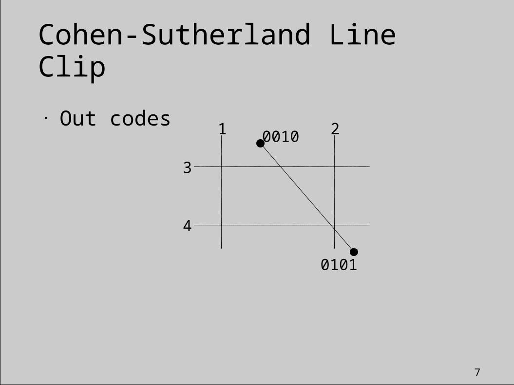
Cohen-Sutherland Line Clip
• Out codes1 2
3
4
0010
0101
8
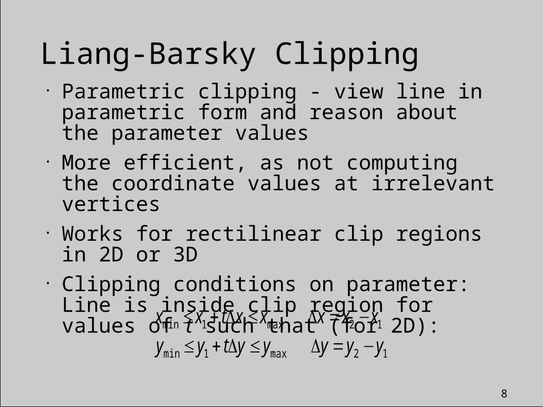
Liang-Barsky Clipping• Parametric clipping - view line in parametric
form and reason about the parameter values• More efficient, as not computing the coordinate
values at irrelevant vertices• Works for rectilinear clip regions in 2D or 3D• Clipping conditions on parameter: Line is inside
clip region for values of t such that (for 2D):
12max1min
12max1min
yyyyytyy
xxxxxtxx
−=Δ≤Δ+≤−=Δ≤Δ+≤

9
Liang-Barsky Clipping
• Infinite line intersects clip region edges at:
k
kk p
qt =
p1 =−Δx q1 =x1 −xmin
p2 =Δx q2 =xmax−x1
p3 =−Δy q3 =y1 −ymin
p4 =Δy q4 =ymax−y1
where
Note: Left edge is 1, right edge is 2, top edge is 3, bottom is 4
10
Liang-Barsky Clipping
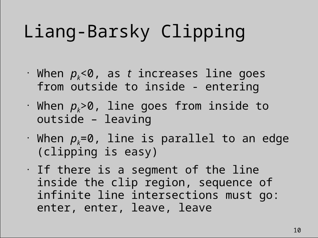
• When pk<0, as t increases line goes from outside to inside - entering
• When pk>0, line goes from inside to outside – leaving
• When pk=0, line is parallel to an edge (clipping is easy)
• If there is a segment of the line inside the clip region, sequence of infinite line intersections must go: enter, enter, leave, leave

11
Liang-Barsky Clipping
Enter Enter
LeaveLeave
Enter
Leave
EnterLeave
12
Liang-Barsky Clipping
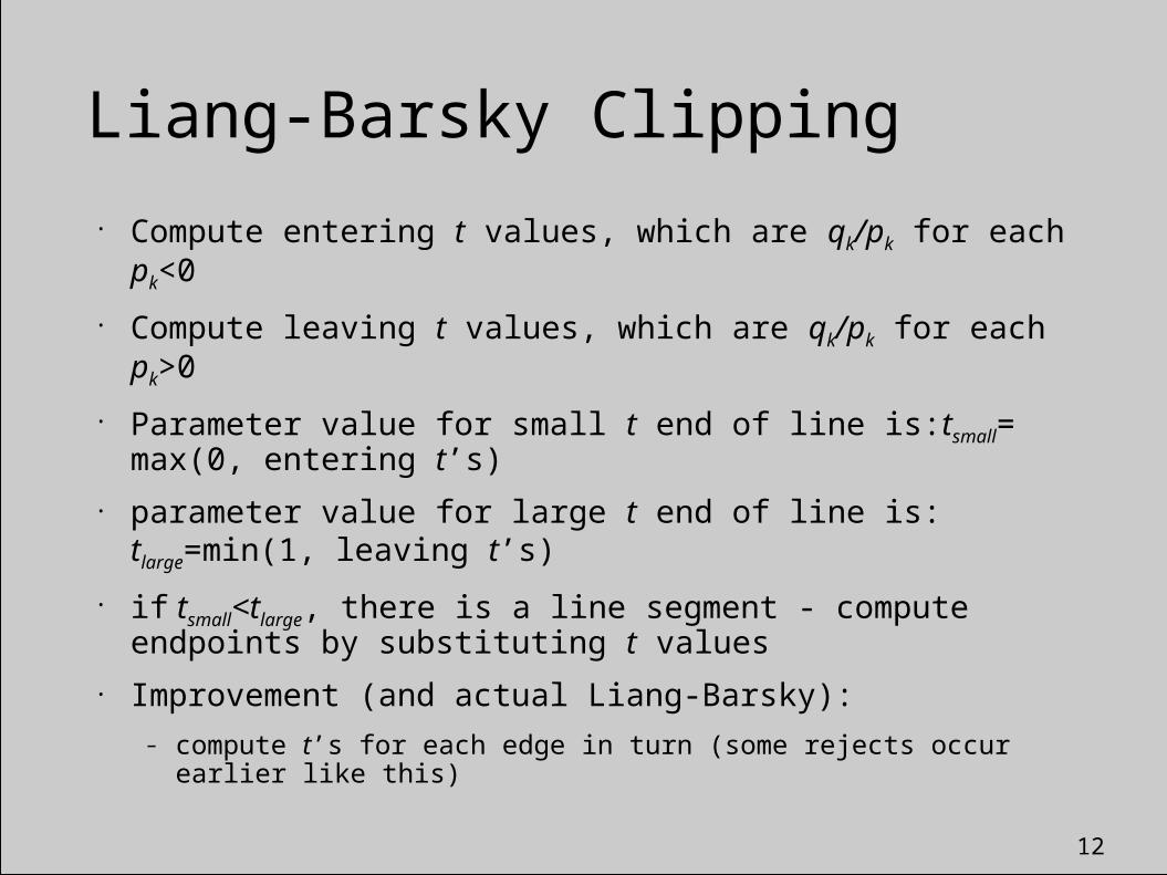
• Compute entering t values, which are qk/pk for each pk<0
• Compute leaving t values, which are qk/pk for each pk>0
• Parameter value for small t end of line is:tsmall= max(0, entering t’s)
• parameter value for large t end of line is: tlarge=min(1, leaving t’s)
• if tsmall<tlarge, there is a line segment - compute endpoints by substituting t values
• Improvement (and actual Liang-Barsky):
– compute t’s for each edge in turn (some rejects occur earlier like this)
13
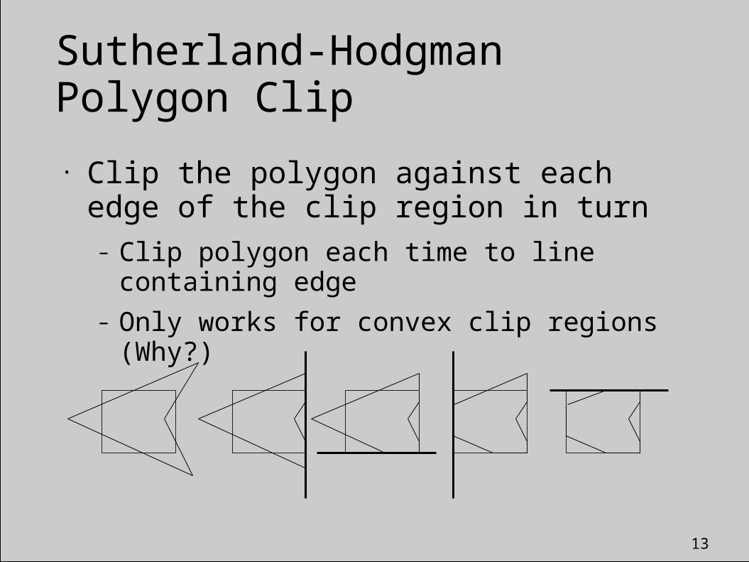
Sutherland-Hodgman Polygon Clip
• Clip the polygon against each edge of the clip region in turn
– Clip polygon each time to line containing edge
– Only works for convex clip regions (Why?)
14
Sutherland-Hodgman Polygon Clip
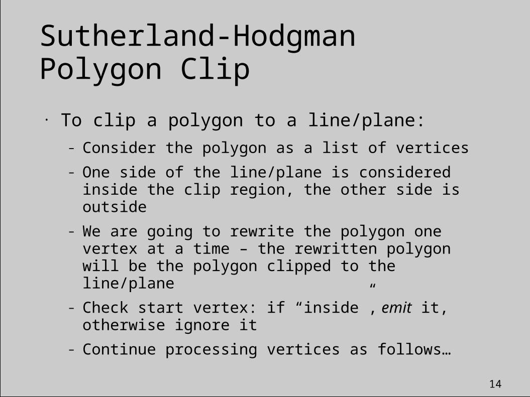
• To clip a polygon to a line/plane:
– Consider the polygon as a list of vertices
– One side of the line/plane is considered inside the clip region, the other side is outside
– We are going to rewrite the polygon one vertex at a time – the rewritten polygon will be the polygon clipped to the line/plane
– Check start vertex: if “inside”, emit it, otherwise ignore it
– Continue processing vertices as follows…

15
Sutherland-Hodgman Polygon Clip
Inside Outside
s
p
Output p
Inside Outside
sp
Output i
Inside Outside
s
p
No output
Inside Outside
sp
Output i and p
i
i

16
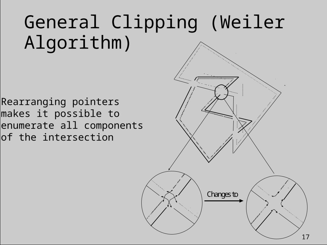
General Clipping (Weiler Algorithm)
17
General Clipping (Weiler Algorithm)
Changes to
Rearranging pointersmakes it possible to enumerate all componentsof the intersection

18
Inside-Outside Testing

19
Inside/Outside in Screen Space
20
Finding Intersection Points

21
Backface Culling

22
Z-Buffer ( a.k.a. Depth Buffer )
• Use additional buffer to store a Z value at each pixel• When filling pixel write Z value to buffer also• Don’t fill if new Z value is larger than old
• Quantization and aliasing problems sometimes occur• Very commonly used• Standard feature in hardware
• Interpolating Z values over polygons

23
Z-Buffer and Transparency
• Must render in order back to front
Partially transparent
Opaque
Opaque 1st
2nd
3rdFront
Good
Partially transparent
Opaque
Opaque 2nd
3rd
1st
Not Good
Talk about compositing later…

24
A-Buffer
• Store list of polygons at each pixel (fragments)• Draw opaque stuff first,only keep closest frag• Second pass for transparent stuff
• Allows antialiasing…
• Not good for hardware implementation
25
Scan Line Algorithm
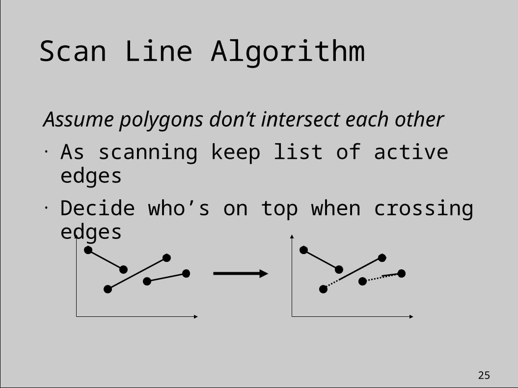
Assume polygons don’t intersect each other• As scanning keep list of active edges• Decide who’s on top when crossing edges

26
Scan Line Algorithm
• Advantages:– Simple– Potentially fewer quantization errors (more bits available for
depth)– Don’t over-render (each pixel only drawn once)– Filter anti-aliasing can be made to work (have information
about all polygons at each pixel)• Disadvantages:
– Invisible polygons clog AEL, ET– Non-intersection criteria may be hard to meet
27
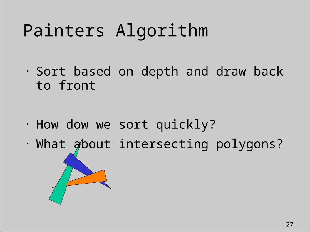
Painters Algorithm
• Sort based on depth and draw back to front
• How dow we sort quickly?• What about intersecting polygons?

28
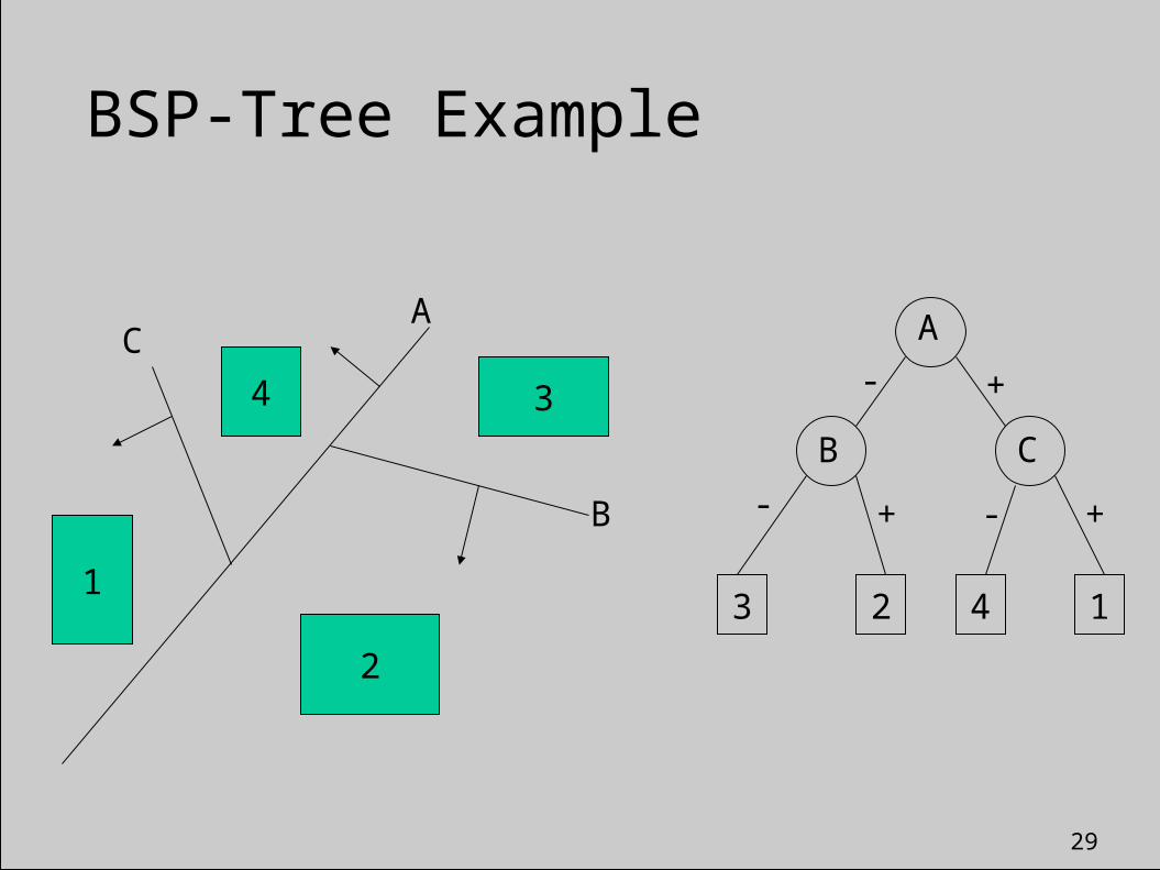
BSP-Trees (Object Precision)
• Construct a binary space partition tree
– Depth-first traversal gives a rendering order (varient)
• Tree splits 3D world with planes
– The world is broken into convex cells
– Each cell is the intersection of all the half-spaces of splitting planes on tree path to the cell
• Also used to model the shape of objects, and in other visibility algorithms
– BSP visibility in games does not necessarily refer to this algorithm
29
BSP-Tree Example
AC
B
2
4
1
3
A
B C
3 2 4 1
-
- -
+
++

30
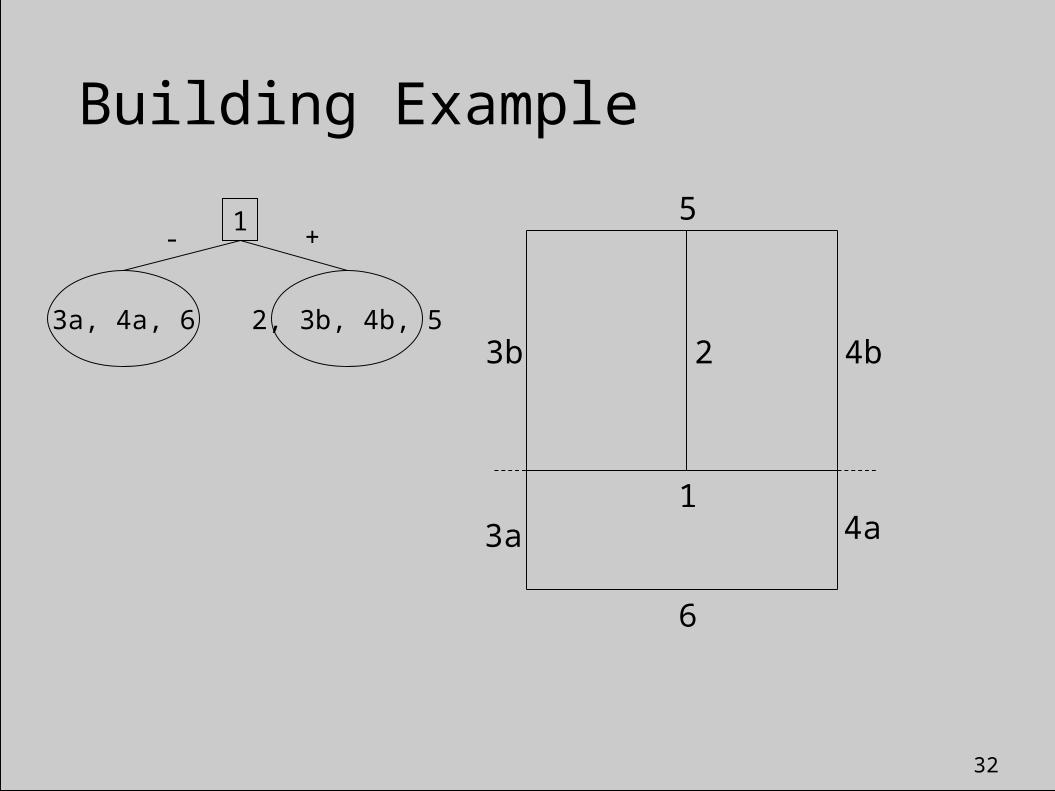
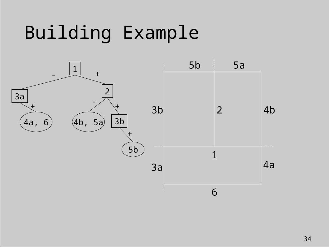
Building BSP-Trees
• Choose polygon (arbitrary)• Split its cell using plane on which polygon lies
– May have to chop polygons in two (Clipping!)• Continue until each cell contains only one polygon
fragment• Splitting planes could be chosen in other ways, but there
is no efficient optimal algorithm for building BSP trees– Optimal means minimum number of polygon fragments in a
balanced tree
31
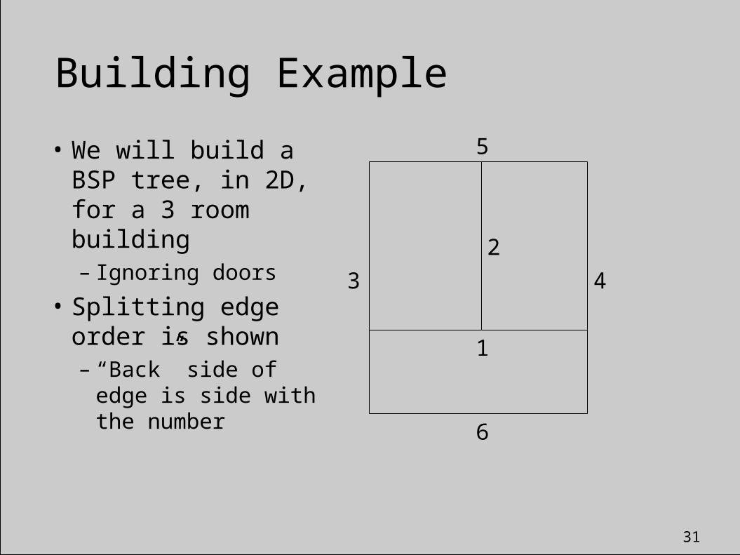
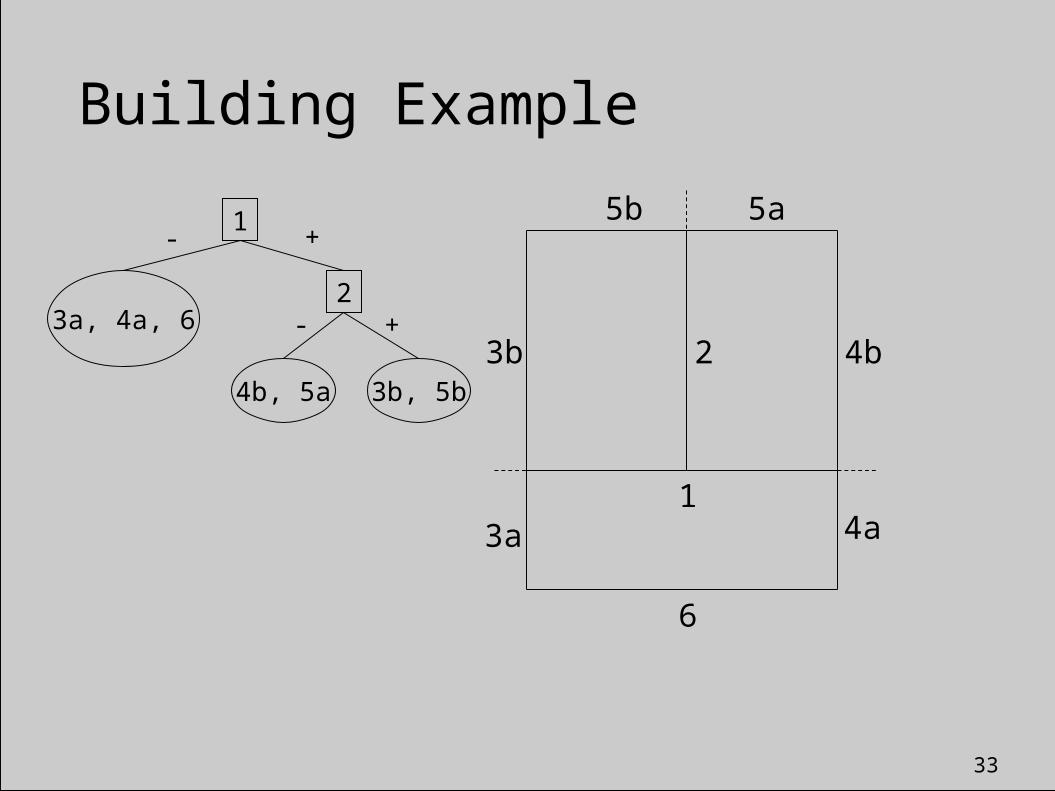
Building Example
• We will build a BSP tree, in 2D, for a 3 room building– Ignoring doors
• Splitting edge order is shown– “Back” side of edge is
side with the number
1
2
3 4
5
6
32
1
23b 4b
5
6
1
3a, 4a, 6 2, 3b, 4b, 5
- +
4a3a
Building Example
33
Building Example
1
23b 4b
5a
6
1
3a, 4a, 6
- +
4a3a
3b, 5b
2
4b, 5a
- +
5b
34
Building Example
1
23b 4b
5a
6
1- +
4a3a
2
4b, 5a
-+
5b
4a, 6
3a+
5b
3b
+
35
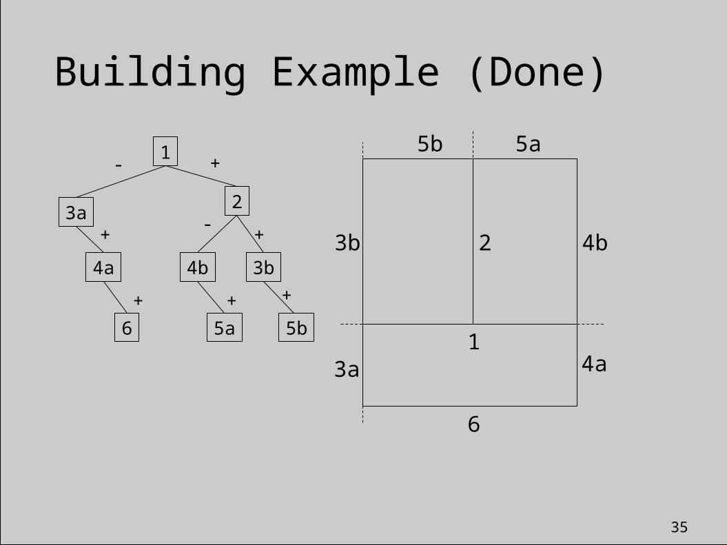
Building Example (Done)
1
23b 4b
5a
6
1- +
4a3a
2-
+
5b
3a+
3b
+
4a
6
+
5b
4b
5a
+
36
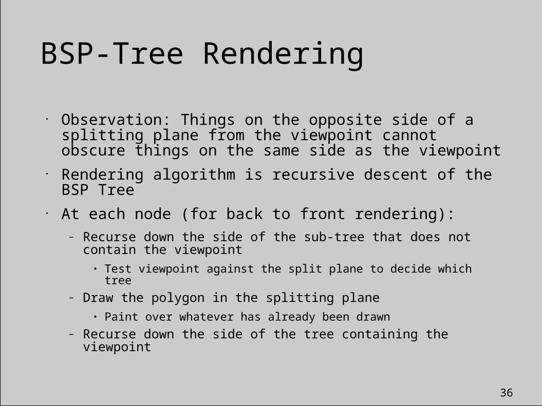
BSP-Tree Rendering
• Observation: Things on the opposite side of a splitting plane from the viewpoint cannot obscure things on the same side as the viewpoint
• Rendering algorithm is recursive descent of the BSP Tree• At each node (for back to front rendering):
– Recurse down the side of the sub-tree that does not contain the viewpoint● Test viewpoint against the split plane to decide which tree
– Draw the polygon in the splitting plane● Paint over whatever has already been drawn
– Recurse down the side of the tree containing the viewpoint

37
BSP-Tree Rendering Example
AC
B
2
4
1
3
A
B C
3 2 4 1
-
- -
+
++
1st 2nd3rd 4th
38
BSP-Tree Rendering
• Advantages:– One tree works for any viewing point
– Filter anti-aliasing and transparency work● Have back to front ordering for compositing
– Can also render front to back, and avoid drawing back polygons that cannot contribute to the view
● User two trees – an extra one that subdivides the window
• Disadvantages:– Can be many small pieces of polygon
39
Cells and Portals
• Assume the world can be broken into cells– Simple shapes
– Rooms in a building, for instance
• Define portals to be the transparent boundaries between cells
– Doorways between rooms, windows, etc
• In a world like this, can determine exactly which parts of which rooms are visible
– Then render visible rooms plus contents• An Exact Visibility Algorithm -- sometimes

40
Cell and Portal Visibility
• Start in the cell containing the viewer, with the full viewing frustum
• Render the walls of that room and its contents• Recursively clip the viewing frustum to each
portal out of the cell, and call the algorithm on the cell beyond the portal

41
Cell-Portal Example
View

42
Cell-Portal Example
View

43
Cell-Portal Example
View

44

45
Acknowledgments
• Some of these slide contents were based on original materials from
– Prof. David Forsyth of U.C. Berkeley
– Prof. Stephen Chenney of U.W. Madison