1

Chapter 11

Neural Networks

2

Chapter 11 Contents (1)

Biological Neurons Artificial Neurons Perceptrons Multilayer Neural Networks Backpropagation

3

Chapter 11 Contents (2)

Recurrent Networks Hopfield Networks Bidirectional Associative Memories Kohonen Maps Hebbian Learning Evolving Neural Networks

4

Biological Neurons

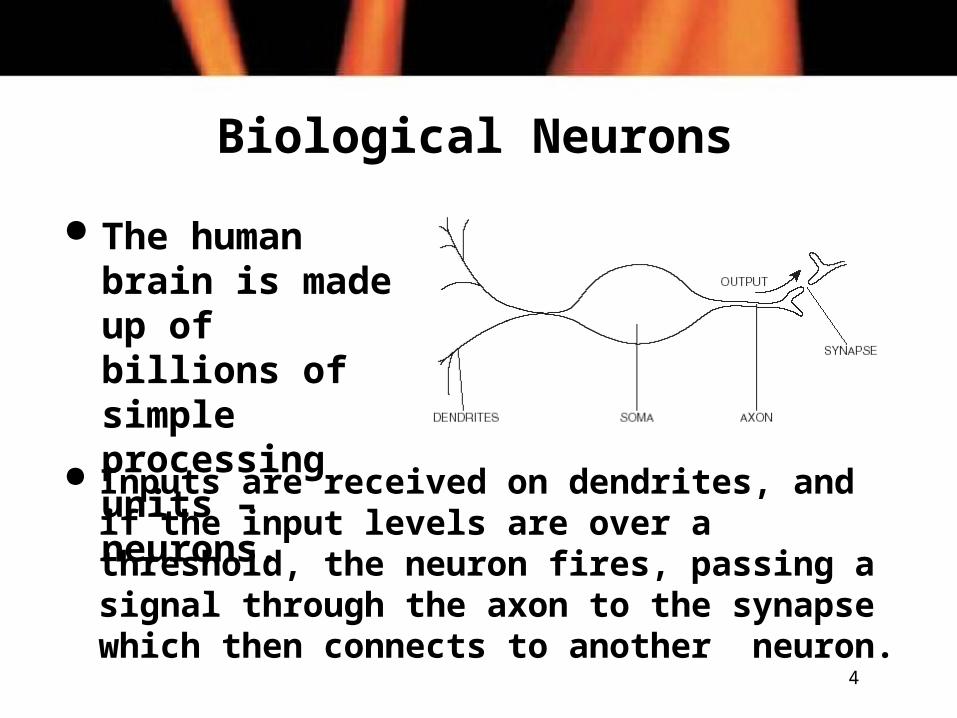
The human brain is made up of billions of simple processing units – neurons.

Inputs are received on dendrites, and if the input levels are over a threshold, the neuron fires, passing a signal through the axon to the synapse which then connects to another neuron.

5

Artificial Neurons (1)

Artificial neurons are based on biological neurons. Each neuron in the network receives one or more

inputs. An activation function is applied to the inputs,

which determines the output of the neuron – the activation level.

The charts on the right show three typical activation functions.

6

Artificial Neurons (2)

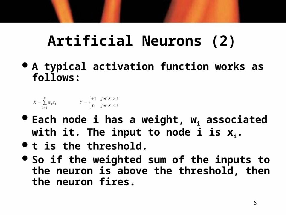
A typical activation function works as follows:

Each node i has a weight, wi associated with it. The input to node i is xi.

t is the threshold. So if the weighted sum of the inputs to the

neuron is above the threshold, then the neuron fires.

7

Perceptrons (1)

A perceptron is a single neuron that classifies a set of inputs into one of two categories (usually 1 or -1).

If the inputs are in the form of a grid, a perceptron can be used to recognize visual images of shapes.

The perceptron usually uses a step function, which returns 1 if the weighted sum of inputs exceeds a threshold, and –1 otherwise.

8

Perceptrons (2)

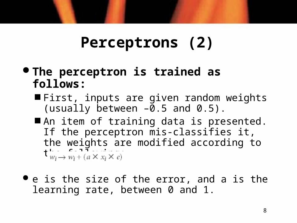
The perceptron is trained as follows: First, inputs are given random weights

(usually between –0.5 and 0.5). An item of training data is presented. If the

perceptron mis-classifies it, the weights are modified according to the following:

e is the size of the error, and a is the learning rate, between 0 and 1.

9

Perceptrons (3)

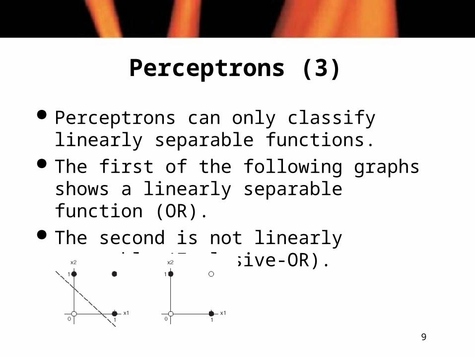
Perceptrons can only classify linearly separable functions.

The first of the following graphs shows a linearly separable function (OR).

The second is not linearly separable (Exclusive-OR).

10

Multilayer Neural Networks

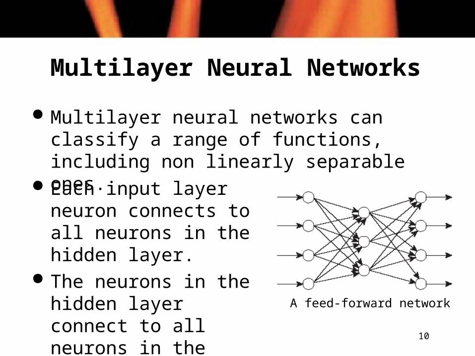
Multilayer neural networks can classify a range of functions, including non linearly separable ones.

Each input layer neuron connects to all neurons in the hidden layer.

The neurons in the hidden layer connect to all neurons in the output layer.

A feed-forward network

11

Backpropagation (1)

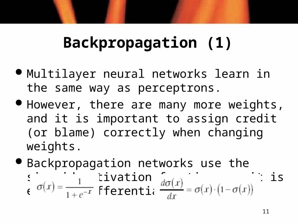
Multilayer neural networks learn in the same way as perceptrons.

However, there are many more weights, and it is important to assign credit (or blame) correctly when changing weights.

Backpropagation networks use the sigmoid activation function, as it is easy to differentiate:

12

Backpropagation (2)

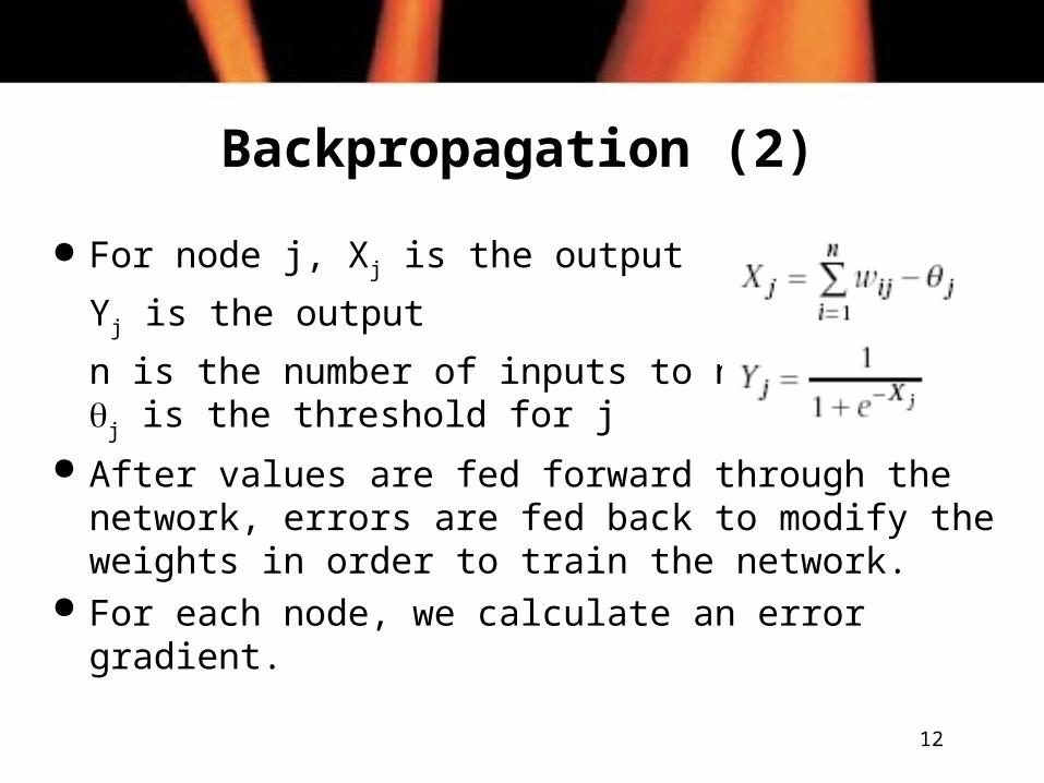
For node j, Xj is the output

Yj is the output

n is the number of inputs to node jj is the threshold for j

After values are fed forward through the network, errors are fed back to modify the weights in order to train the network.

For each node, we calculate an error gradient.

13

Backpropagation (3)

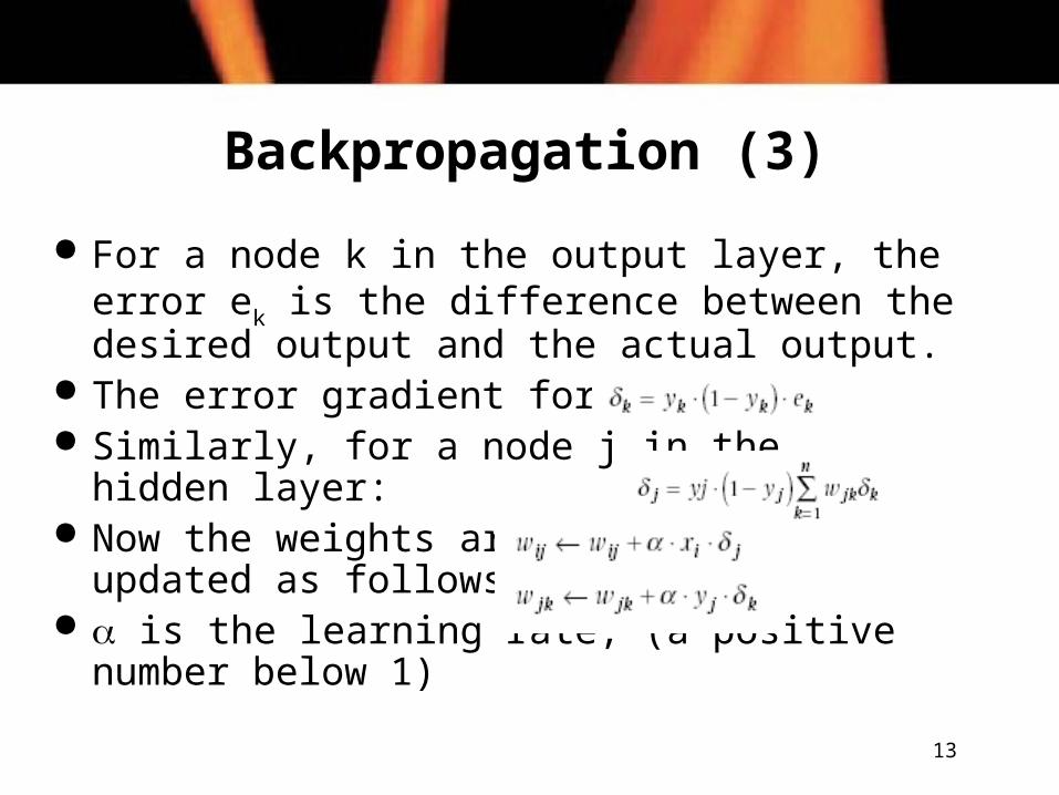
For a node k in the output layer, the error ek is the difference between the desired output and the actual output.

The error gradient for k is: Similarly, for a node j in the

hidden layer: Now the weights are

updated as follows: is the learning rate, (a positive number

below 1)

14

Recurrent Networks

Feed forward networks do not have memory.

Recurrent networks can have connections between nodes in any layer, which enables them to store data – a memory.

Recurrent networks can be used to solve problems where the solution depends on previous inputs as well as current inputs (e.g. predicting stock market movements).

15

Hopfield Networks A Hopfield Network is a recurrent network. Use a sign activation function: If a neuron receives a 0 as an input it does not change

state. Inputs are usually represented as matrices. The network is trained to represent a set of attractors,

or stable states. Any input will be mapped to an output state which is

the attractor closest to the input. A Hopfield network is autoassociative – it can only

associate an item with itself or a similar one.

16

Bidirectional Associative Memories

A BAM is a heteroassociative memory: Like the brain, it can learn to

associate one item with another completely unrelated item.

The network consists of two fully connected layers of nodes – every node in one layer is connected to every node in the other layer.

17

Kohonen Maps An unsupervised learning system. Two layers of nodes: an input layer and a

cluster (output) layer. Uses competitive learning:

Every input is compared with the weight vectors of each node in the cluster node.

The node which most closely matches the input, fires. This is the classification of the input.

Euclidean distance is used. The winning node has its weight vector modified to be

closer to the input vector.

18

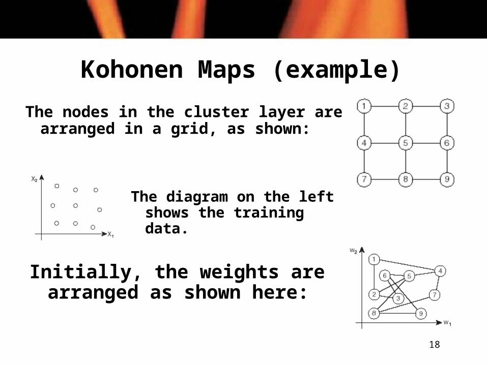
Kohonen Maps (example)

Initially, the weights are arranged as shown here:

The diagram on the left shows the training data.

The nodes in the cluster layer are arranged in a grid, as shown:

19

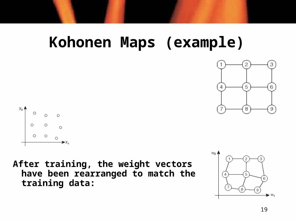
Kohonen Maps (example)

After training, the weight vectors have been rearranged to match the training data:

20

Hebbian Learning (1)

Hebb’s law:“When an axon of cell A is near enough to excite

a cell B and repeatedly or persistently takes part in firing it, some growth process or metabolic change takes place in one or both cells such that A’s efficiency, as one of the cells firing B, is increased”.

Hence, if two neurons that are connected together fire at the same time, the weights of the connection between them is strengthened.

21

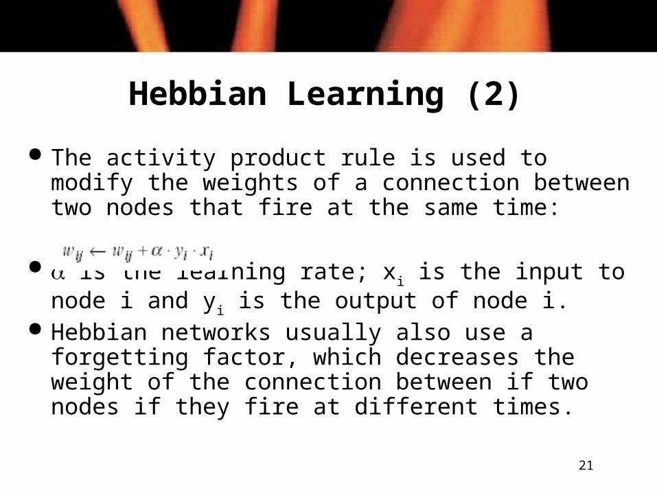
Hebbian Learning (2)

The activity product rule is used to modify the weights of a connection between two nodes that fire at the same time:

is the learning rate; xi is the input to node i and yi is the output of node i.

Hebbian networks usually also use a forgetting factor, which decreases the weight of the connection between if two nodes if they fire at different times.

22

Evolving Neural Networks

Neural networks can be susceptible to local maxima.

Evolutionary methods (genetic algorithms) can be used to determine the starting weights for a neural network, thus avoiding these kinds of problems.