1

Chapter 11

A number of important scheduling problems . . . require the study of an astronomical number of arrangements to determine which one is best. . . . Mathematicians have been working on improved techniques.-- George Dantzig

Integer and Goal Programming

2

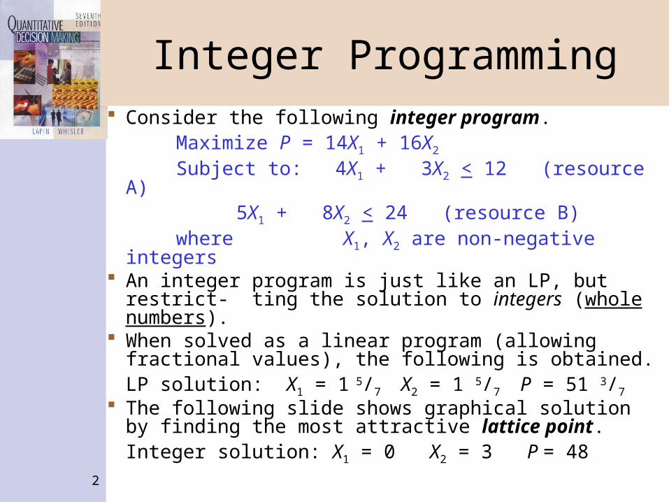
Integer Programming Consider the following integer program. Maximize P = 14X1 + 16X2

Subject to: 4X1 + 3X2 < 12 (resource A) 5X1 + 8X2 < 24 (resource B) where X1, X2 are non-negative integers An integer program is just like an LP, but restrict- ting

the solution to integers (whole numbers). When solved as a linear program (allowing fractional

values), the following is obtained.LP solution: X1 = 1 5/7 X2 = 1 5/7 P = 51 3/7

The following slide shows graphical solution by finding the most attractive lattice point.

Integer solution: X1 = 0 X2 = 3 P = 48

3

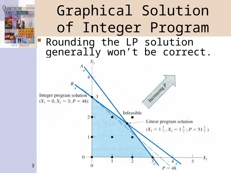
Graphical Solutionof Integer Program

Rounding the LP solution generally won’t be correct.

4

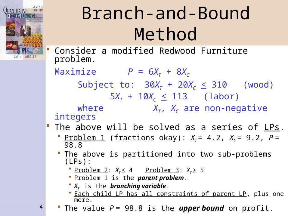
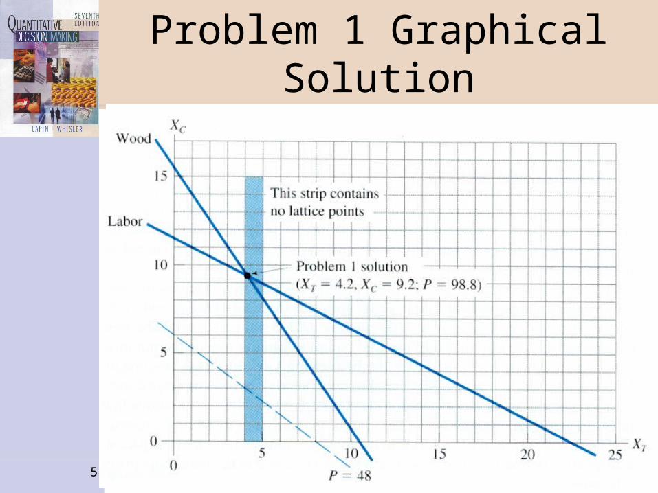
Branch-and-Bound Method Consider a modified Redwood Furniture problem.

Maximize P = 6XT + 8XC

Subject to: 30XT + 20XC < 310 (wood) 5XT + 10XC < 113 (labor) where XT, XC are non-negative integers The above will be solved as a series of LPs.

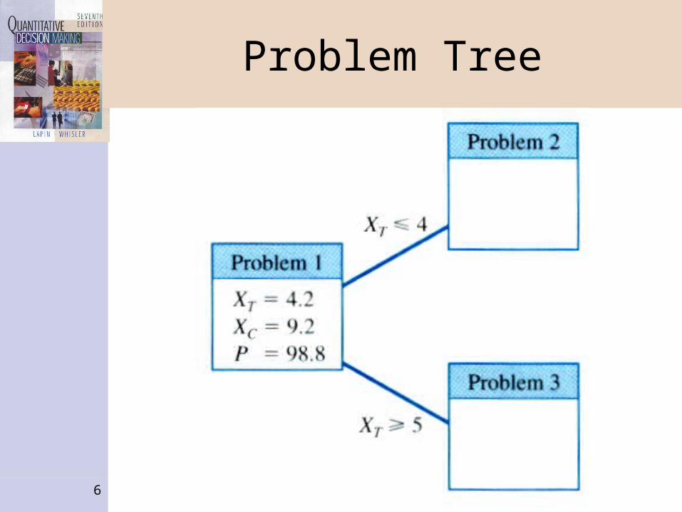
Problem 1 (fractions okay): XT = 4.2, XC = 9.2, P = 98.8 The above is partitioned into two sub-problems (LPs):

Problem 2: XT < 4 Problem 3: XT > 5 Problem 1 is the parent problem. XT is the branching variable. Each child LP has all constraints of parent LP, plus one more.

The value P = 98.8 is the upper bound on profit.

5

Problem 1 Graphical Solution

6

Problem Tree

7

Graphical Solutions toProblems 2 and 3

8

The Problem Tree The problem tree gives the genealogy of the LPs

being solved. Each child LP is defined by a constraint involving the

branching variable, chosen (arbitrarily) because its value is non-integer.

One child has constraint: branching variable < (largest integer < current value) The sibling has constraint: branching variable > (smallest integer > current value) None of the problems have integer restrictions.

Solutions will be found however in which all variables happen to have integers.

The P of the child LP can never be better than that of its parent. Do you know why?

9

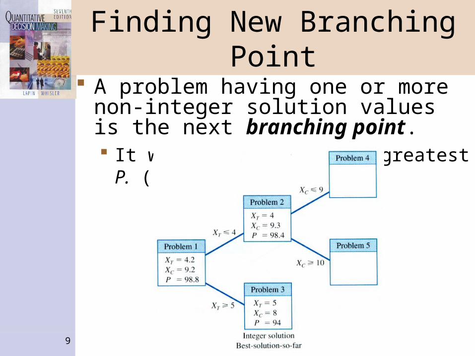
Finding New Branching Point

A problem having one or more non-integer solution values is the next branching point. It will be the one with greatest P. (Problem 2)

10

Best-Solution-So-Far

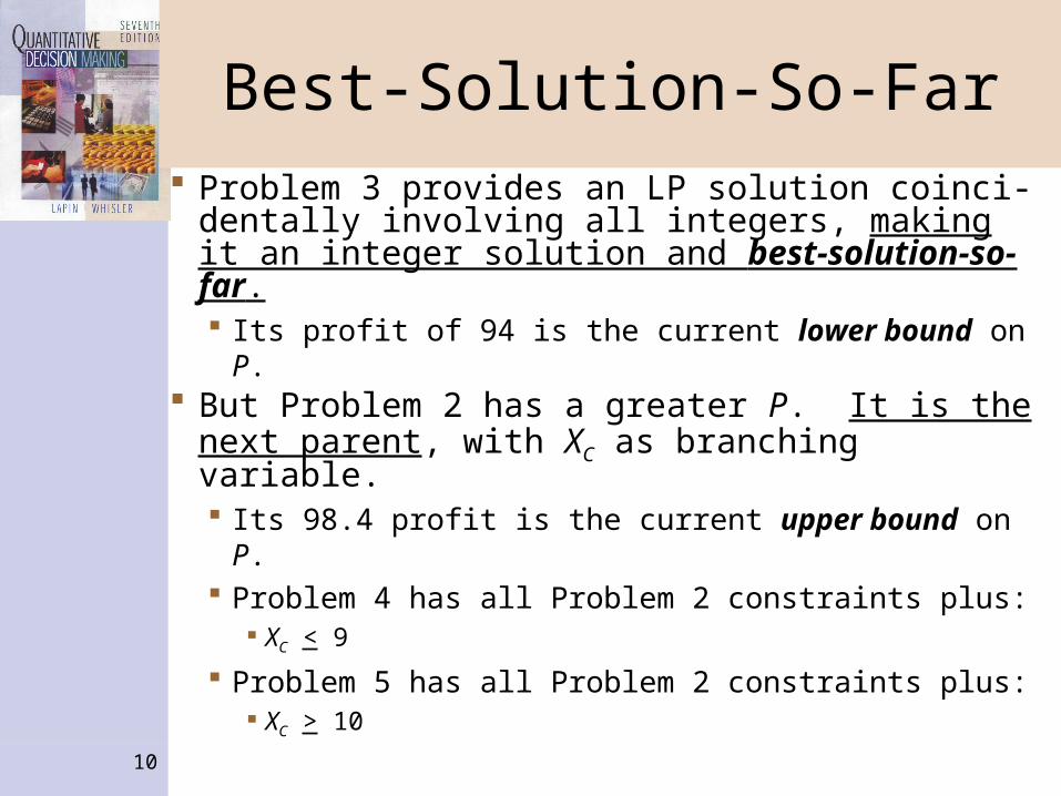
Problem 3 provides an LP solution coinci- dentally involving all integers, making it an integer solution and best-solution-so-far. Its profit of 94 is the current lower bound on P.

But Problem 2 has a greater P. It is the next parent, with XC as branching variable. Its 98.4 profit is the current upper bound on P. Problem 4 has all Problem 2 constraints plus:

XC < 9

Problem 5 has all Problem 2 constraints plus: XC > 10

11

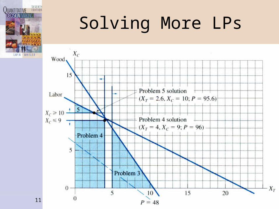
Solving More LPs

12

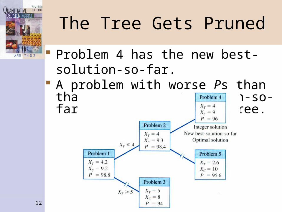
The Tree Gets Pruned

Problem 4 has the new best-solution-so-far. A problem with worse Ps than that of the

best-solution-so-far is pruned from the tree.

13

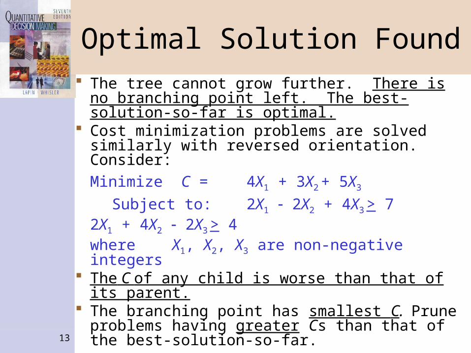
Optimal Solution Found The tree cannot grow further. There is no

branching point left. The best-solution-so-far is optimal.

Cost minimization problems are solved similarly with reversed orientation. Consider:

Minimize C = 4X1 + 3X2 + 5X3

Subject to: 2X1 2X2 + 4X3 > 72X1 + 4X2 2X3 > 4

where X1, X2, X3 are non-negative integers The C of any child is worse than that of its parent. The branching point has smallest C. Prune

problems having greater Cs than that of the best-solution-so-far.

14

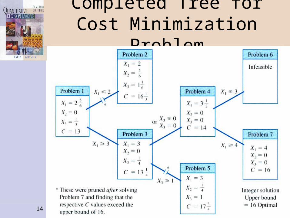
Completed Tree forCost Minimization Problem

15

Solving Integer Programswith QuickQuant

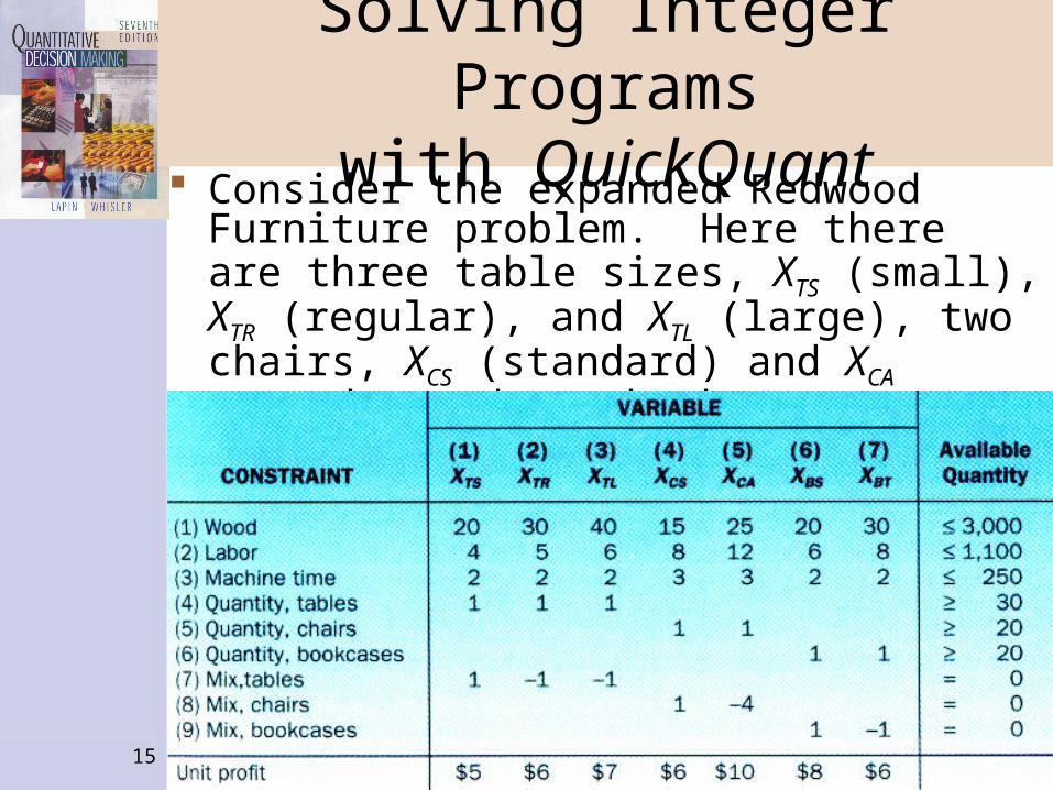
Consider the expanded Redwood Furniture problem. Here there are three table sizes, XTS (small), XTR (regular), and XTL (large), two chairs, XCS (standard) and XCA (armed), and two bookcases, XBS (short) and XBT (tall).

16

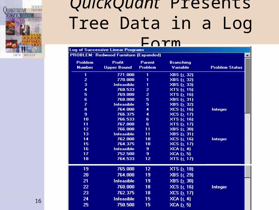
QuickQuant Presents Tree Data in a Log Form

17

Solution to ExpandedRedwood Furniture Problem

18

Linear Programmingwith Multiple Objectives

Linear programming has a single objective function. That may be inadequate because: Two or more goals might apply simultaneously.

Investors try to maximize return and minimize risk. Objectives can conflict, as with the above. Each objective may have a different solution.

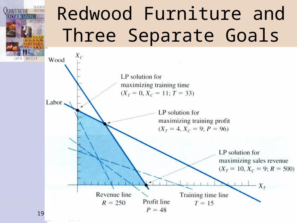
Consider the original Redwood Furniture problem, with the following objectives. 1. Maximize P = 6XT + 8XC (profit) 2. Maximize R = 50XT + 25XC (revenue) 3. Maximize T = 1XT + 3XC (training time)

19

Redwood Furniture andThree Separate Goals

20

Goal Programming

Linear programming may be adapted to treat multiple goals simultaneously.

The procedure is called goal programming. It begins with goal targets:

1. Profit $ 90 2. Sales revenue $ 450 3. Training time 30 hours

For some goals, exceeding the target is desirable. For others, lying below is better. And, closeness to target (above or below) may be important.

21

Goal Programming Extra goal deviation variables convert the LP to a

goal program. These are weighted according to their relative importance. YP

+,YP = deviation of profit above, below target

YR+,YR

= deviation of revenue above, below target YT

+,YT = deviation of training time above, below target

The goals are incorporated into an omnibus objective function minimizing collective weighted deviations from respective targets.

The resulting goal program has the original constraints and goal deviation constraints. 1. 6XT + 8XC (YP

+ YP) = 90 (profit)

2. 50XT + 25XC (YR+ YR

) = 450 (revenue) 3. 1XT + 3XC (YT

+ YT) = 30 (training)

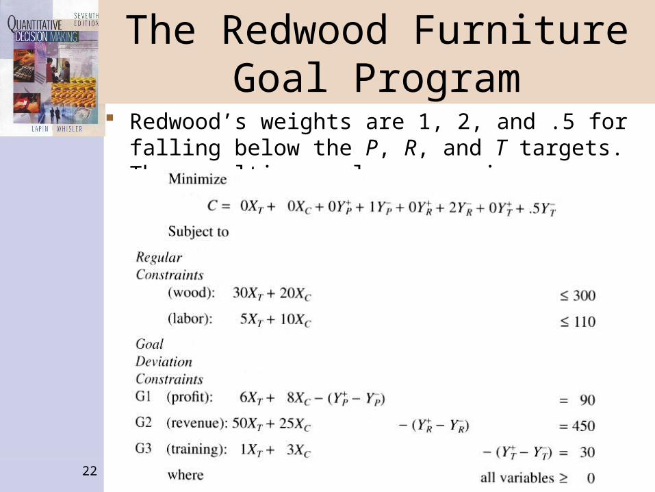
22

The Redwood FurnitureGoal Program

Redwood’s weights are 1, 2, and .5 for falling below the P, R, and T targets. The resulting goal program is:

23

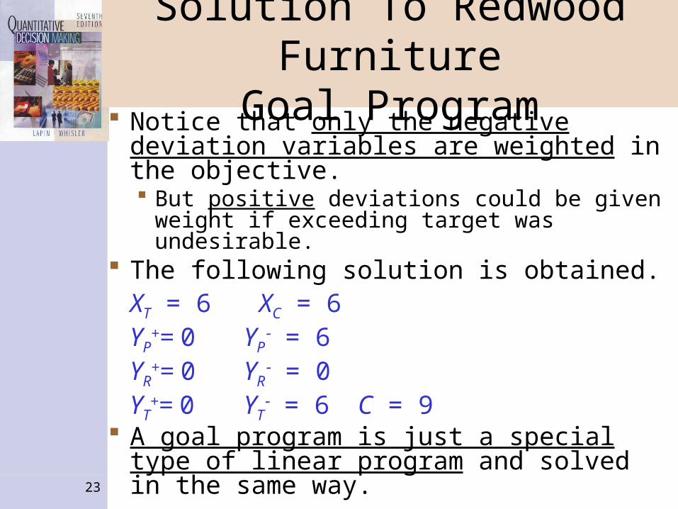
Solution To Redwood FurnitureGoal Program

Notice that only the negative deviation variables are weighted in the objective. But positive deviations could be given weight if

exceeding target was undesirable. The following solution is obtained.

XT = 6 XC = 6YP

+= 0 YP = 6

YR+= 0 YR

= 0 YT

+= 0 YT = 6 C = 9

A goal program is just a special type of linear program and solved in the same way.

24

Solving Integer Programswith Spreadsheets

Spreadsheets can be used to solve integer programs just like they are used to solve linear programs.

25

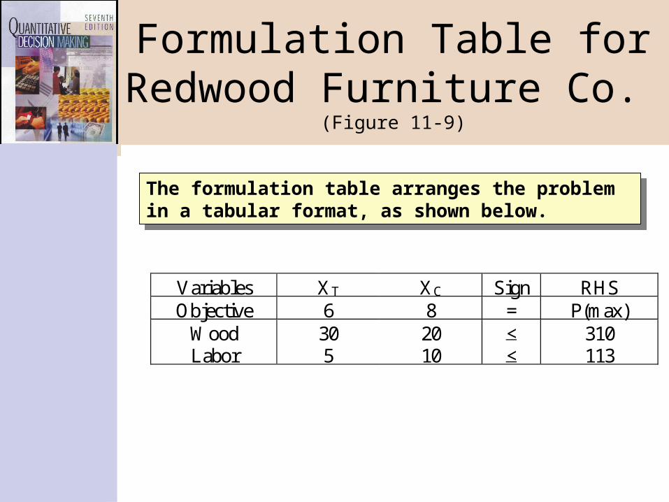
Formulation Table for Redwood Furniture Co. (Figure 11-9)

Variables XT XC Sign RHSObjective 6 8 = P(max)

WoodLabor

305

2010

<<

310113

The formulation table arranges the problem in a tabular format, as shown below.

The formulation table arranges the problem in a tabular format, as shown below.

26

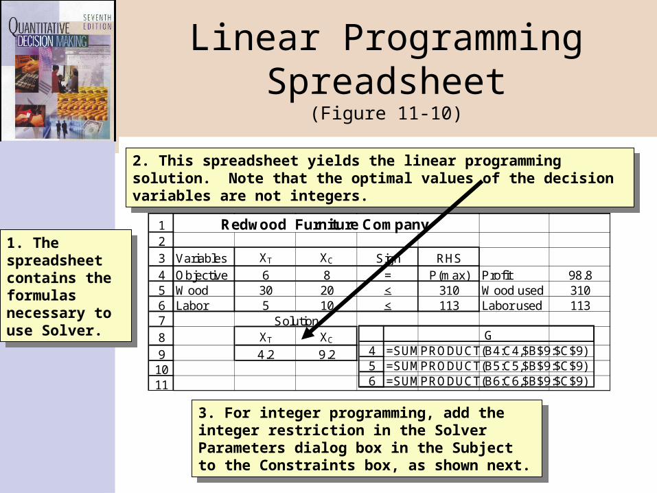
Linear Programming Spreadsheet(Figure 11-10)

123456789

1011

A B C D E F G

Redwood Furniture Company

Variables XT XC Sign RHSObjective 6 8 = P(max) Profit 98.8Wood 30 20 < 310 Wood used 310Labor 5 10 < 113 Labor used 113

XT XC

4.2 9.2

Solution

456

G=SUMPRODUCT(B4:C4,$B$9:$C$9)=SUMPRODUCT(B5:C5,$B$9:$C$9)=SUMPRODUCT(B6:C6,$B$9:$C$9)

3. For integer programming, add the integer restriction in the Solver Parameters dialog box in the Subject to the Constraints box, as shown next.

3. For integer programming, add the integer restriction in the Solver Parameters dialog box in the Subject to the Constraints box, as shown next.

2. This spreadsheet yields the linear programming solution. Note that the optimal values of the decision variables are not integers.

2. This spreadsheet yields the linear programming solution. Note that the optimal values of the decision variables are not integers.

1. The spreadsheet contains the formulas necessary to use Solver.

1. The spreadsheet contains the formulas necessary to use Solver.

27

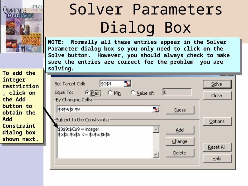
Solver Parameters Dialog Box(Figure 11-11)

To add the integer restriction, click on the Add button to obtain the Add Constraint dialog box shown next.

To add the integer restriction, click on the Add button to obtain the Add Constraint dialog box shown next.

NOTE: Normally all these entries appear in the Solver Parameter dialog box so you only need to click on the Solve button. However, you should always check to make sure the entries are correct for the problem you are solving.

NOTE: Normally all these entries appear in the Solver Parameter dialog box so you only need to click on the Solve button. However, you should always check to make sure the entries are correct for the problem you are solving.

28

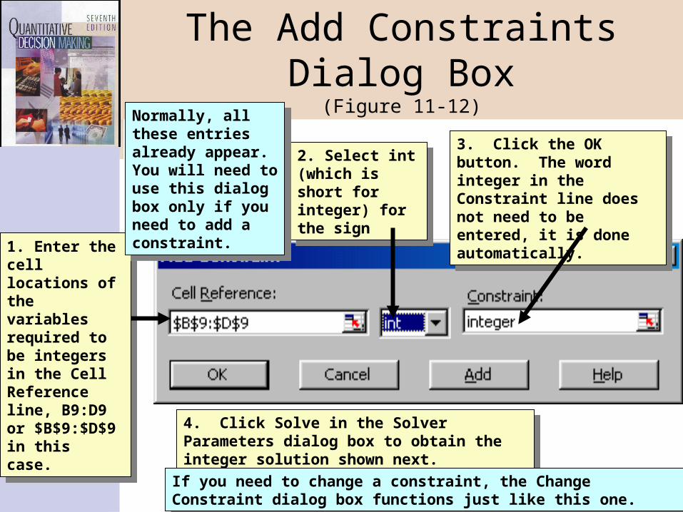
The Add Constraints Dialog Box(Figure 11-12)

1. Enter the cell locations of the variables required to be integers in the Cell Reference line, B9:D9 or $B$9:$D$9 in this case.

1. Enter the cell locations of the variables required to be integers in the Cell Reference line, B9:D9 or $B$9:$D$9 in this case.

2. Select int (which is short for integer) for the sign

2. Select int (which is short for integer) for the sign

3. Click the OK button. The word integer in the Constraint line does not need to be entered, it is done automatically.

3. Click the OK button. The word integer in the Constraint line does not need to be entered, it is done automatically.

4. Click Solve in the Solver Parameters dialog box to obtain the integer solution shown next.

4. Click Solve in the Solver Parameters dialog box to obtain the integer solution shown next.

Normally, all these entries already appear. You will need to use this dialog box only if you need to add a constraint.

Normally, all these entries already appear. You will need to use this dialog box only if you need to add a constraint.

If you need to change a constraint, the Change Constraint dialog box functions just like this one.

If you need to change a constraint, the Change Constraint dialog box functions just like this one.

29

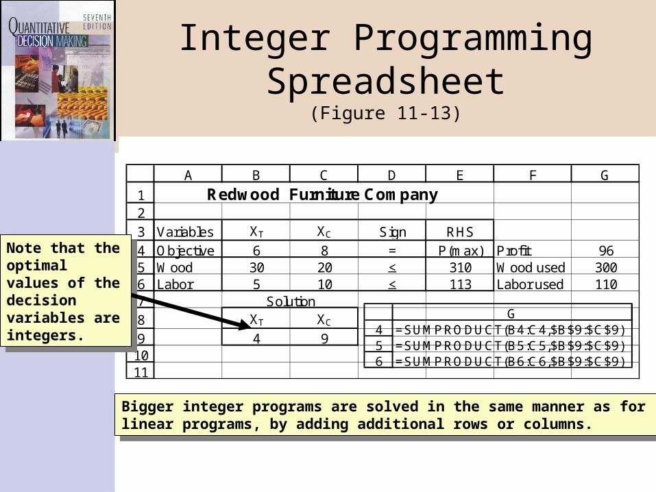
Integer Programming Spreadsheet(Figure 11-13)

123456789

1011

A B C D E F G

Redwood Furniture Company

Variables XT XC Sign RHSObjective 6 8 = P(max) Profit 96Wood 30 20 < 310 Wood used 300Labor 5 10 < 113 Labor used 110

XT XC

4 9

Solution

456

G=SUMPRODUCT(B4:C4,$B$9:$C$9)=SUMPRODUCT(B5:C5,$B$9:$C$9)=SUMPRODUCT(B6:C6,$B$9:$C$9)

Bigger integer programs are solved in the same manner as for linear programs, by adding additional rows or columns.

Bigger integer programs are solved in the same manner as for linear programs, by adding additional rows or columns.

Note that the optimal values of the decision variables are integers.

Note that the optimal values of the decision variables are integers.

30

Solving Goal Programswith Spreadsheets

Spreadsheets can be used to solve goal programs just like they are used to solve linear programs.

31

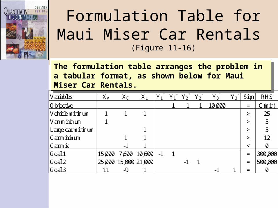
Formulation Table forMaui Miser Car Rentals (Figure 11-16)

Variables XV XC XL Y1+ Y1

- Y2+ Y2

- Y3+ Y3

- Sign RHS

Objective 1 1 1 10,000 = C(min)Vehicle minimum 1 1 1 > 25Van minimum 1 > 5Large car minimum 1 > 5Car minimum 1 1 > 12Car mix -1 1 < 0Goal 1 15,000 7,600 10,600 -1 1 = 300,000Goal 2 25,000 15,000 21,000 -1 1 = 500,000Goal 3 11 -9 1 -1 1 = 0

The formulation table arranges the problem in a tabular format, as shown below for Maui Miser Car Rentals.

The formulation table arranges the problem in a tabular format, as shown below for Maui Miser Car Rentals.

32

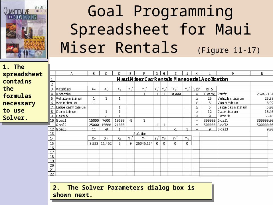
Goal Programming Spreadsheet for Maui Miser Rentals (Figure 11-17)

123

456789

1011121314

1516171819202122

A B C D E F G H I J K L M N

Variables XV XC XL Y1+ Y1

- Y2+ Y2

- Y3+ Y3

-Sign RHS

Objective 1 1 1 10,000 = C(min) Profit 26046.154Vehicle minimum 1 1 1 > 25 Vehicle minimum 25.38Van minimum 1 > 5 Van minimum 8.92Large car minimum 1 > 5 Large car minimum 5.00Car minimum 1 1 > 12 Car minimum 16.46Car mix -1 1 < 0 Car mix -6.46Goal 1 15000 7600 10600 -1 1 = 300000 Goal 1 300000.00Goal 2 25000 15000 21000 -1 1 = 500000 Goal 2 500000.00Goal 3 11 -9 1 -1 1 = 0 Goal 3 0.00

XV XC XL Y1+ Y1

- Y2+ Y2

- Y3+ Y3

-

8.923 11.462 5 0 26046.154 0 0 0 0

Maui Miser Car Rentals Managerial Application

Solution

456789

101112

N=SUMPRODUCT(B4:J4,$B$15:$J$15)=SUMPRODUCT(B5:J5,$B$15:$J$15)=SUMPRODUCT(B6:J6,$B$15:$J$15)=SUMPRODUCT(B7:J7,$B$15:$J$15)=SUMPRODUCT(B8:J8,$B$15:$J$15)=SUMPRODUCT(B9:J9,$B$15:$J$15)=SUMPRODUCT(B10:J10,$B$15:$J$15)=SUMPRODUCT(B11:J11,$B$15:$J$15)=SUMPRODUCT(B12:J12,$B$15:$J$15)

1. The spreadsheet contains the formulas necessary to use Solver.

1. The spreadsheet contains the formulas necessary to use Solver.

2. The Solver Parameters dialog box is shown next.2. The Solver Parameters dialog box is shown next.

33

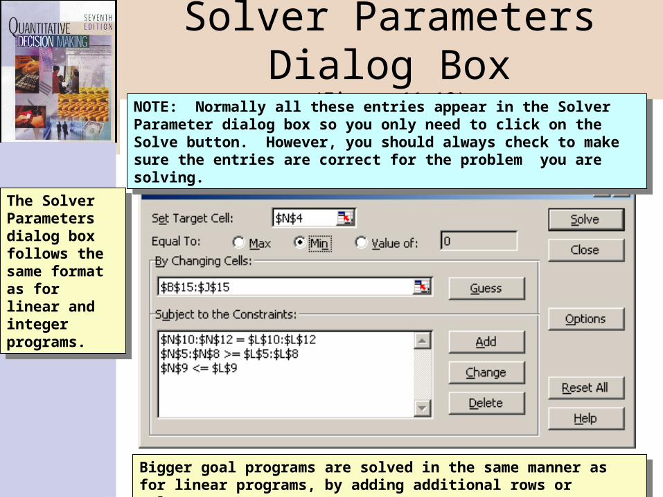
Solver Parameters Dialog Box(Figure 11-18)

Bigger goal programs are solved in the same manner as for linear programs, by adding additional rows or columns.

Bigger goal programs are solved in the same manner as for linear programs, by adding additional rows or columns.

The Solver Parameters dialog box follows the same format as for linear and integer programs.

The Solver Parameters dialog box follows the same format as for linear and integer programs.

NOTE: Normally all these entries appear in the Solver Parameter dialog box so you only need to click on the Solve button. However, you should always check to make sure the entries are correct for the problem you are solving.

NOTE: Normally all these entries appear in the Solver Parameter dialog box so you only need to click on the Solve button. However, you should always check to make sure the entries are correct for the problem you are solving.