1(c) 1999-2007, I.P.L. Png & D.E. Lehman

Outline

Own-price elasticity Forecasting quantity demanded and

expenditure Other elasticities Adjustment time

2(c) 1999-2007, I.P.L. Png & D.E. Lehman

Own-price elasticity

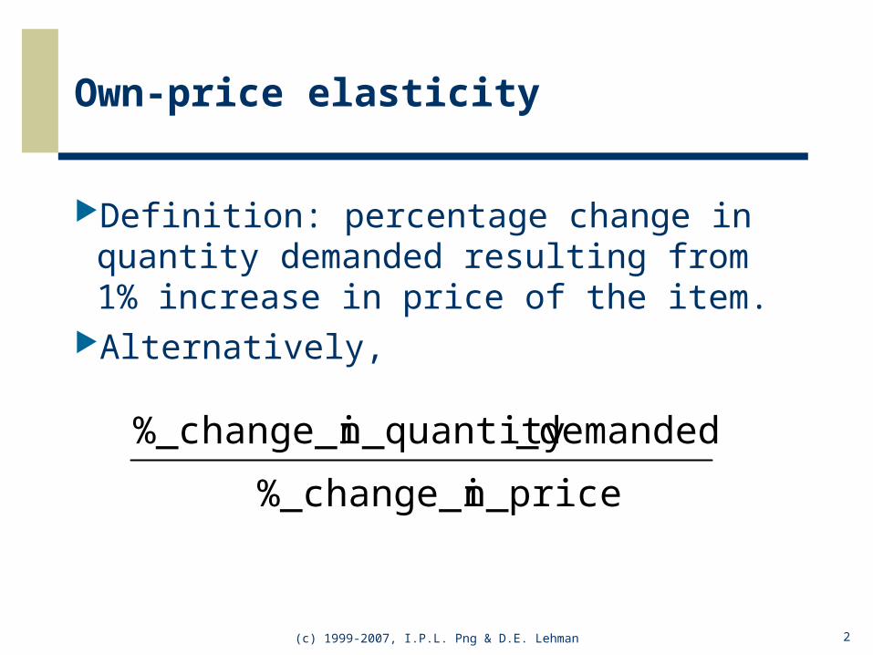
Definition: percentage change in quantity demanded resulting from 1% increase in price of the item.

Alternatively,

n_price%_change_i

_demandedn_quantity%_change_i

Own-price elasticity: Calculation

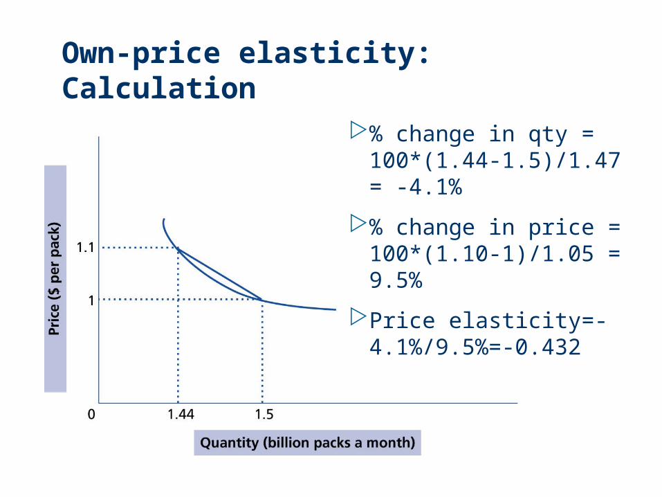
% change in qty = 100*(1.44-1.5)/1.47 = -4.1%

% change in price = 100*(1.10-1)/1.05 = 9.5%

Price elasticity=-4.1%/9.5%=-0.432

4(c) 1999-2007, I.P.L. Png & D.E. Lehman

Own-price elasticity

Elasticity: 1% price increase leads to more than 1% drop in quantity demanded.

Inelastic: 1% price increase leads to less than 1% drop in quantity demanded.

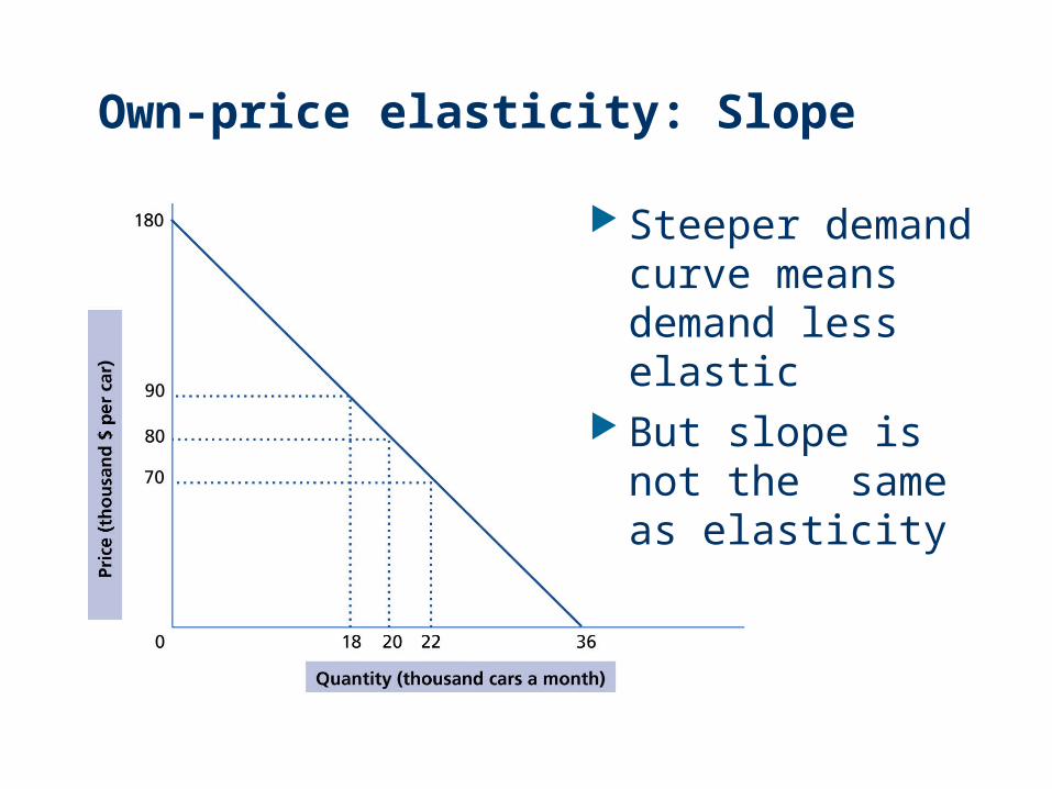
Own-price elasticity: Slope

Steeper demand curve means demand less elastic

But slope is not the same as elasticity

Own-price elasticity“ Extensive research and many years of experience have taught us that business travel demand is quite inelastic… On the other hand, pleasure travel has substantial elasticity.”Robert L. Crandall, CEO, American Airlines, 1989

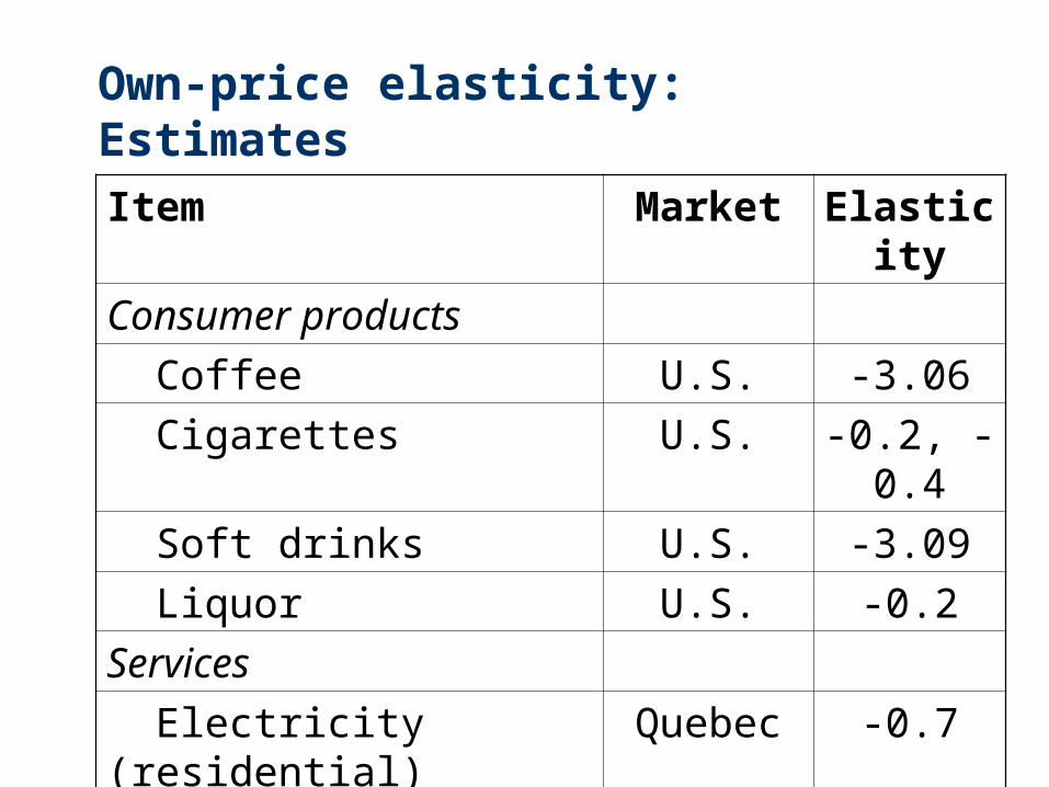
Own-price elasticity:EstimatesItem Market Elastici

ty

Consumer products

Coffee U.S. -3.06

Cigarettes U.S. -0.2, -0.4

Soft drinks U.S. -3.09

Liquor U.S. -0.2

Services

Electricity (residential) Quebec -0.7

Water (residential) U.S. [-0.2, -0.3]

Water (industrial) U.S. [-0.7, -1.0]

8(c) 1999-2007, I.P.L. Png & D.E. Lehman

Own-price elasticity: Factors

Availability of substitutes Cost / benefit of economizing – buyer’s

“involvement”

9(c) 1999-2007, I.P.L. Png & D.E. Lehman

Own-price elasticity: Factors

Buyer’s prior commitments Learning: Apple or Dell complementary purchases: printer and

inkjet cartridges Taste: baby formula Through smart business strategy: in

1981, American Airlines pioneered frequent flyer program, which became very attractive to business travelers

10(c) 1999-2007, I.P.L. Png & D.E. Lehman

Outline

Own-price elasticity Forecasting quantity demanded

and expenditure Other elasticities Adjustment time

11(c) 1999-2007, I.P.L. Png & D.E. Lehman

Forecasting:When to raise price

CEO: “Profits are low. We must raise prices.”

Sales Manager: “But my sales would fall!”

Real issue: How sensitive are buyers to price changes?

12(c) 1999-2007, I.P.L. Png & D.E. Lehman

Forecasting

Forecasting quantity demanded Change in quantity demanded = price

elasticity of demand x change in price

13(c) 1999-2007, I.P.L. Png & D.E. Lehman

Forecasting:Price increase

If demand elastic, price increase leads to proportionately greater reduction in

purchases lower total sales revenue (sales

revenue=price*quantity demanded) If demand inelastic, price increase leads to

proportionately smaller reduction in purchases

higher total sales revenue

14(c) 1999-2007, I.P.L. Png & D.E. Lehman

Forecasting:Price increase

If demand inelastic, price increase leads to proportionately smaller reduction in

purchases higher expenditure = higher sales

revenue Lower sales lower cost higher profit

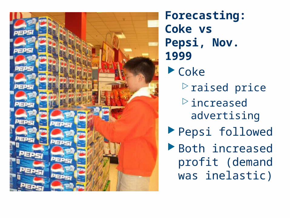
Forecasting:Coke vs Pepsi, Nov. 1999

Coke raised price increased

advertising Pepsi followed Both increased

profit (demand was inelastic)

16(c) 1999-2007, I.P.L. Png & D.E. Lehman

Outline

Own-price elasticity Forecasting quantity demanded and

expenditure Other elasticities Adjustment time

17(c) 1999-2007, I.P.L. Png & D.E. Lehman

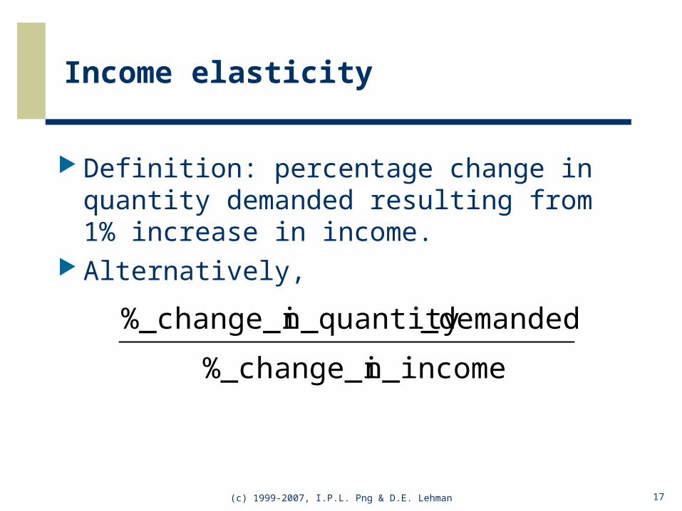
Income elasticity

Definition: percentage change in quantity demanded resulting from 1% increase in income.

Alternatively,

n_income%_change_i

_demandedn_quantity%_change_i

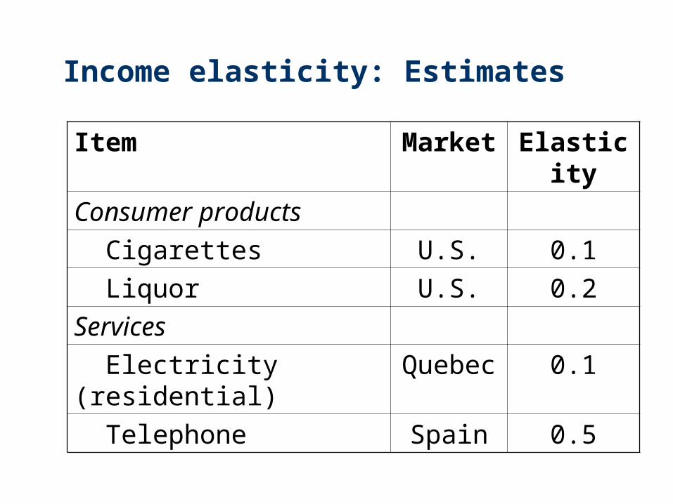
Income elasticity: Estimates

Item Market

Elasticity

Consumer products

Cigarettes U.S. 0.1

Liquor U.S. 0.2

Services

Electricity (residential)

Quebec 0.1

Telephone Spain 0.5

19(c) 1999-2007, I.P.L. Png & D.E. Lehman

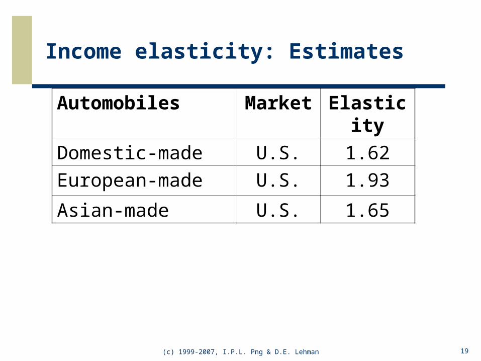
Income elasticity: Estimates

Automobiles Market

Elasticity

Domestic-made U.S. 1.62

European-made U.S. 1.93

Asian-made U.S. 1.65

20(c) 1999-2007, I.P.L. Png & D.E. Lehman

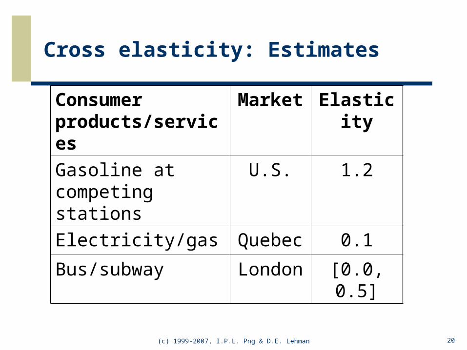
Cross elasticity: Estimates

Consumer products/services

Market

Elasticity

Gasoline at competing stations

U.S. 1.2

Electricity/gas Quebec 0.1

Bus/subway London [0.0, 0.5]

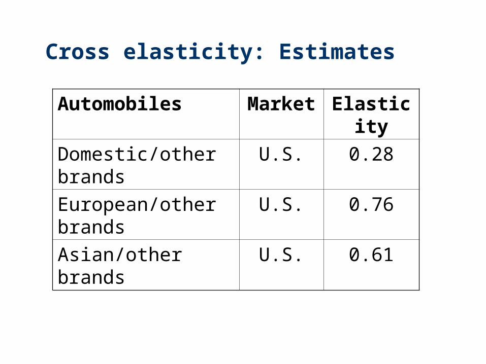
Cross elasticity: Estimates

Automobiles Market

Elasticity

Domestic/other brands

U.S. 0.28

European/other brands

U.S. 0.76

Asian/other brands

U.S. 0.61

22(c) 1999-2007, I.P.L. Png & D.E. Lehman

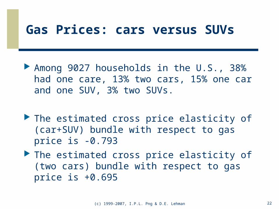
Gas Prices: cars versus SUVs

Among 9027 households in the U.S., 38% had one care, 13% two cars, 15% one car and one SUV, 3% two SUVs.

The estimated cross price elasticity of (car+SUV) bundle with respect to gas price is -0.793

The estimated cross price elasticity of (two cars) bundle with respect to gas price is +0.695

23(c) 1999-2007, I.P.L. Png & D.E. Lehman

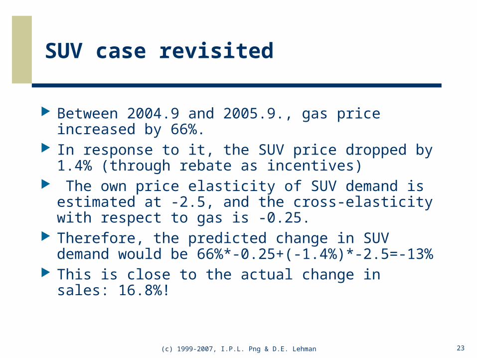
SUV case revisited

Between 2004.9 and 2005.9., gas price increased by 66%.

In response to it, the SUV price dropped by 1.4% (through rebate as incentives)

The own price elasticity of SUV demand is estimated at -2.5, and the cross-elasticity with respect to gas is -0.25.

Therefore, the predicted change in SUV demand would be 66%*-0.25+(-1.4%)*-2.5=-13%

This is close to the actual change in sales: 16.8%!

Advertising elasticity

direct effect – raises demand

indirect effect – makes demand less sensitive to price

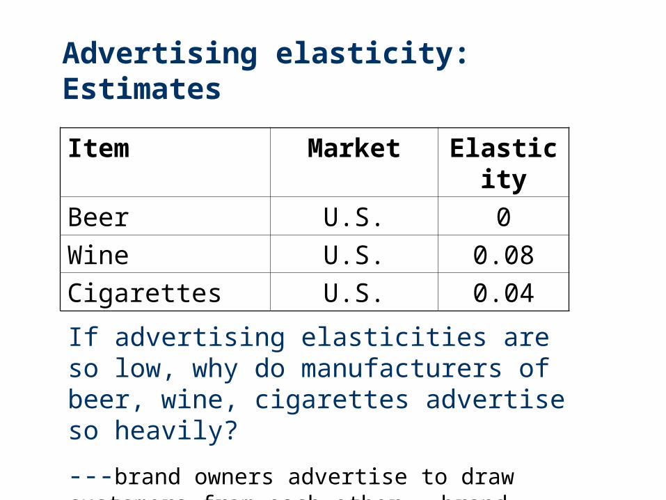
Advertising elasticity: Estimates

Item Market Elasticity

Beer U.S. 0

Wine U.S. 0.08

Cigarettes U.S. 0.04

If advertising elasticities are so low, why do manufacturers of beer, wine, cigarettes advertise so heavily?

---brand owners advertise to draw customers from each other – brand-level demand is more sensitive to advertising

26(c) 1999-2007, I.P.L. Png & D.E. Lehman

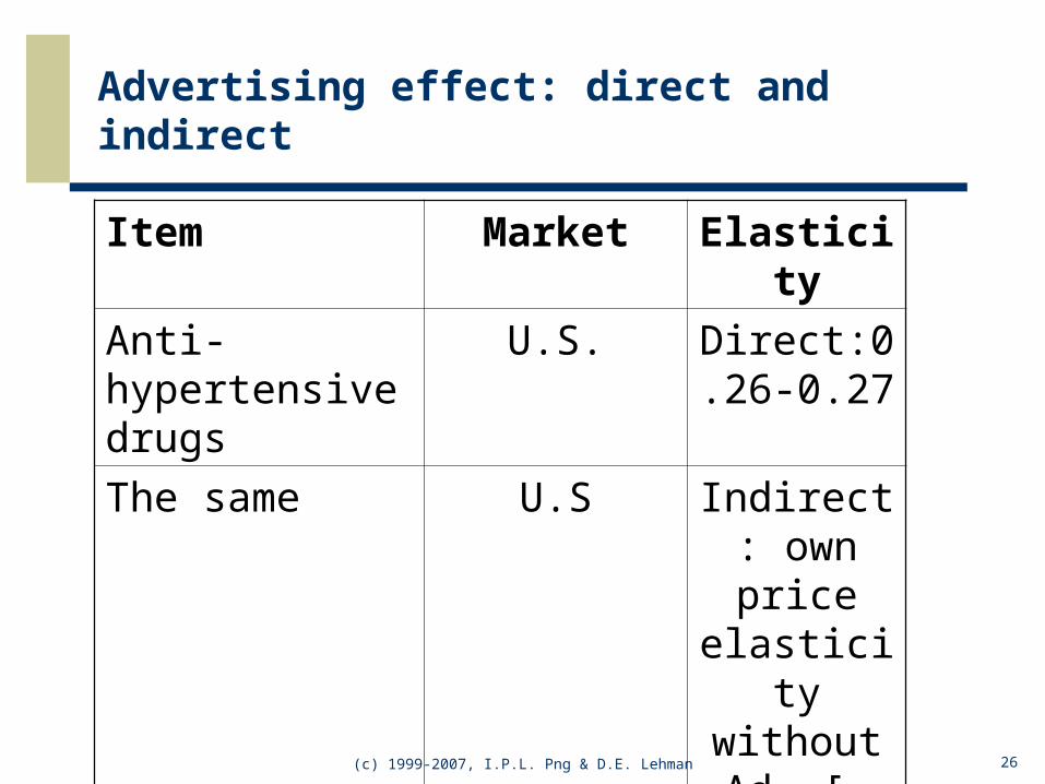
Advertising effect: direct and indirect

Item Market Elasticity

Anti-hypertensive drugs

U.S. Direct:0.26-0.27

The same U.S Indirect: own price elasticity without Ad. [-

2.1,-2.0]

The same U.S. Indirect: own price elasticity with Ad.[-1.7, -

1.5]

27(c) 1999-2007, I.P.L. Png & D.E. Lehman

Outline

Own-price elasticity Forecasting quantity demanded and

expenditure Other elasticities Adjustment time

28(c) 1999-2007, I.P.L. Png & D.E. Lehman

Adjustment time

Definitions Short run: buyer cannot adjust at least

one item of consumption or usage Long run: long enough time for buyer to

adjust all items

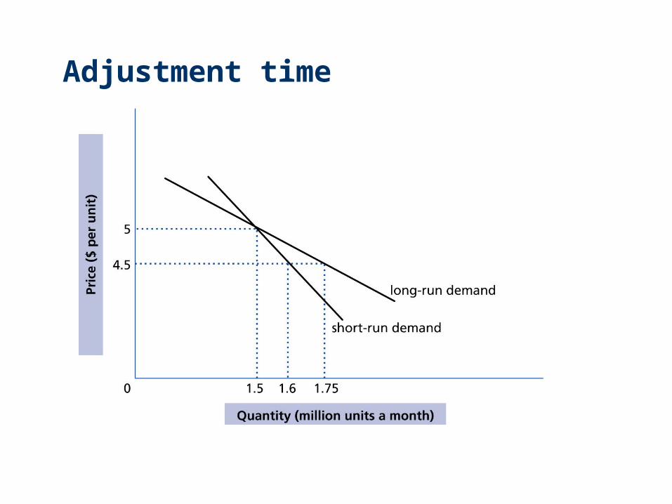
Adjustment time

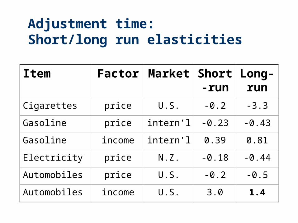
Adjustment time:Short/long run elasticities

Item Factor Market

Short-run

Long-run

Cigarettes price U.S. -0.2 -3.3

Gasoline price intern’l -0.23 -0.43

Gasoline income intern’l 0.39 0.81

Electricity price N.Z. -0.18 -0.44

Automobiles price U.S. -0.2 -0.5

Automobiles income U.S. 3.0 1.4

31(c) 1999-2007, I.P.L. Png & D.E. Lehman

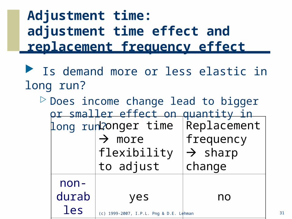
Adjustment time:adjustment time effect and replacement frequency effect

Longer time more flexibility to adjust

Replacement frequency sharp change

non-durabl

esyes no

durables

yes yes

Is demand more or less elastic in long run?

Does income change lead to bigger or smaller effect on quantity in long run?

32(c) 1999-2007, I.P.L. Png & D.E. Lehman

Summary

Own-price elasticity Forecasting quantity demanded and

expenditure Other elasticities Adjustment time

33(c) 1999-2007, I.P.L. Png & D.E. Lehman

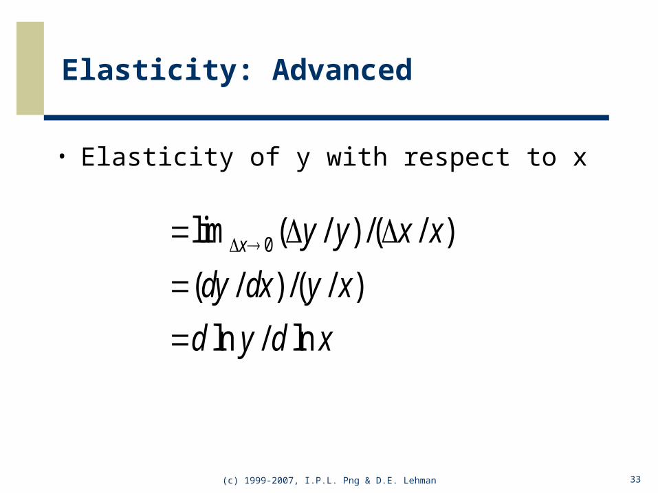
Elasticity: Advanced

• Elasticity of y with respect to x

0lim ( / ) /( / )

( / ) /( / )

ln / ln

x y y x x

dy dx y x

d y d x

34(c) 1999-2007, I.P.L. Png & D.E. Lehman

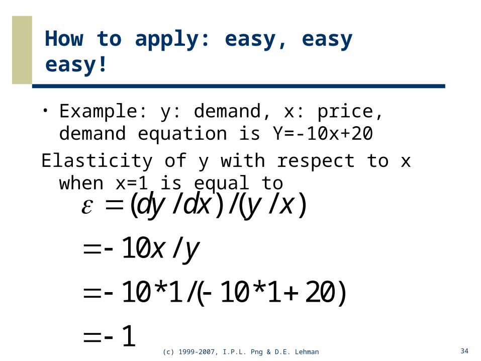
How to apply: easy, easy easy!

• Example: y: demand, x: price, demand equation is Y=-10x+20

Elasticity of y with respect to x when x=1 is equal to

( / ) /( / )

10 /

10*1/( 10*1 20)

1

dy dx y x

x y

35(c) 1999-2007, I.P.L. Png & D.E. Lehman

Brain Tweezing

Elasticity is different at different x’s. Try x=0.5 and try x=1.5 and see it

yourself!

36(c) 1999-2007, I.P.L. Png & D.E. Lehman

Brain Tweezing: How to forecast the impact of price change?

Assume: Y=a*x+b We don’t know a and b We can estimate a and b using historical

sales data: simple regressions. Then we can calculate the elasticity at

any level of x. Finally, we can forecast the impact of

price change on y and the total sales revenue y*x!