Dendrite Spacings in Directionally Solidified Superalloy ...
Upload
bryan-elmer-reynoldsCategory
view
218download
0
1
At the dendrite the incomingsignals arrive (incoming currents)
Molekules
Synapses
Neurons
Local Nets
Areas
Systems
CNS
At the soma currentare finally integrated.
At the axon hillock action potentialare generated if the potential crosses the membrane threshold
The axon transmits (transports) theaction potential to distant sites
At the synapses are the outgoing signals transmitted onto the dendrites of the target neurons
Structure of a Neuron:

2
Chemical synapse:Learning = Change of Synaptic Strength
NeurotransmitterReceptors

3
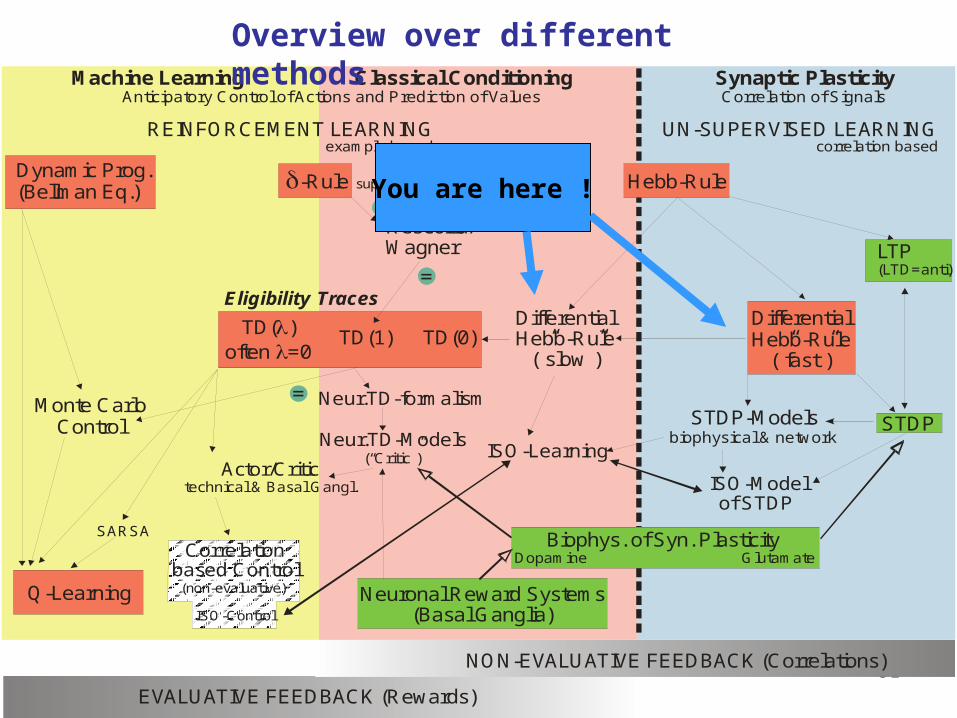
Machine Learning Classical Conditioning Synaptic Plasticity
Dynamic Prog.(Bellman Eq.)
REINFORCEMENT LEARNING UN-SUPERVISED LEARNINGexample based correlation based
d-Rule
Monte CarloControl
Q-Learning
TD( )often =0
ll
TD(1) TD(0)
Rescorla/Wagner
Neur.TD-Models(“Critic”)
Neur.TD-formalism
DifferentialHebb-Rule
(”fast”)
STDP-Modelsbiophysical & network
EVALUATIVE FEEDBACK (Rewards)
NON-EVALUATIVE FEEDBACK (Correlations)
SARSA
Correlationbased Control
(non-evaluative)
ISO-Learning
ISO-Modelof STDP
Actor/Critictechnical & Basal Gangl.
Eligibility Traces
Hebb-Rule
DifferentialHebb-Rule
(”slow”)
supervised L.
Anticipatory Control of Actions and Prediction of Values Correlation of Signals
=
=
=
Neuronal Reward Systems(Basal Ganglia)
Biophys. of Syn. PlasticityDopamine Glutamate
STDP
LTP(LTD=anti)
ISO-Control
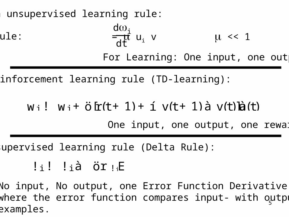
Overview over different methods

4
Different Types/Classes of Learning
Unsupervised Learning (non-evaluative feedback)
• Trial and Error Learning.
• No Error Signal.
• No influence from a Teacher, Correlation evaluation only.
Reinforcement Learning (evaluative feedback)
• (Classic. & Instrumental) Conditioning, Reward-based Lng.
• “Good-Bad” Error Signals.
• Teacher defines what is good and what is bad.
Supervised Learning (evaluative error-signal feedback)
• Teaching, Coaching, Imitation Learning, Lng. from examples and more.
• Rigorous Error Signals.
• Direct influence from a teacher/teaching signal.
5
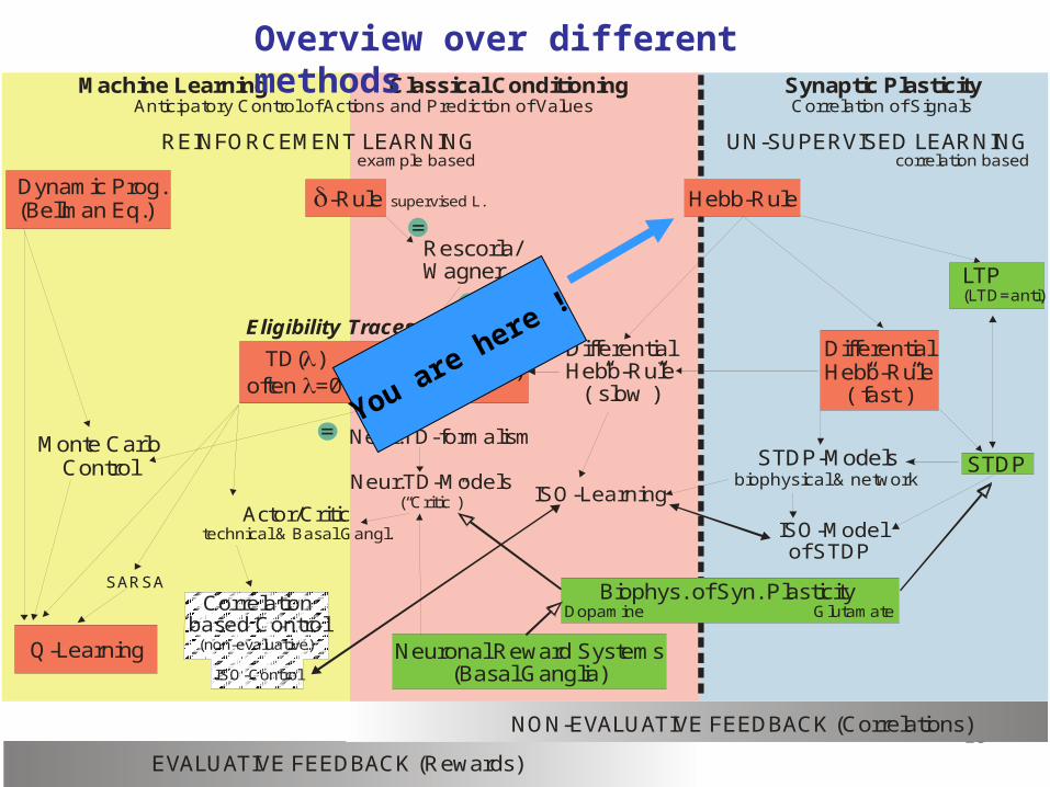
Basic Hebb-Rule: = ui v << 1di
dt
For Learning: One input, one output.
An unsupervised learning rule:
A supervised learning rule (Delta Rule):
! i ! ! i à ör ! iE
No input, No output, one Error Function Derivative,where the error function compares input- with output-examples.
A reinforcement learning rule (TD-learning):
One input, one output, one reward.
wi ! wi + ö[r(t + 1) + í v(t + 1) à v(t)]uà(t)

6
map
Self-organizing maps:unsupervised learning
Neighborhood relationships are usually preserved (+)
Absolute structure depends on initial condition and cannot be predicted (-)
input

7
Basic Hebb-Rule: = ui v << 1di
dt
For Learning: One input, one output
An unsupervised learning rule:
A supervised learning rule (Delta Rule):
! i ! ! i à ör ! iE
No input, No output, one Error Function Derivative,where the error function compares input- with output-examples.
A reinforcement learning rule (TD-learning):
One input, one output, one reward
wi ! wi + ö[r(t + 1) + í v(t + 1) à v(t)]uà(t)

8
I. Pawlow
Classical Conditioning

9
Basic Hebb-Rule: = ui v << 1di
dt
For Learning: One input, one output
An unsupervised learning rule:
A supervised learning rule (Delta Rule):
! i ! ! i à ör ! iE
No input, No output, one Error Function Derivative,where the error function compares input- with output-examples.
A reinforcement learning rule (TD-learning):
One input, one output, one reward
wi ! wi + ö[r(t + 1) + í v(t + 1) à v(t)]uà(t)

10
Supervised Learning: Example OCR

11
The influence of the type of learning on speed and autonomy of the learner
Correlation based learning: No teacher
Reinforcement learning , indirect influence
Reinforcement learning, direct influence
Supervised Learning, Teacher
Programming
Learning Speed Autonomy

12
Hebbian learning
AB
A
B
t
When an axon of cell A excites cell B and repeatedly or persistently takes part in firing it, some growth processes or metabolic change takes place in one or both cells so that A‘s efficiency ... is increased.
Donald Hebb (1949)
13
Machine Learning Classical Conditioning Synaptic Plasticity
Dynamic Prog.(Bellman Eq.)
REINFORCEMENT LEARNING UN-SUPERVISED LEARNINGexample based correlation based
d-Rule
Monte CarloControl
Q-Learning
TD( )often =0
ll
TD(1) TD(0)
Rescorla/Wagner
Neur.TD-Models(“Critic”)
Neur.TD-formalism
DifferentialHebb-Rule
(”fast”)
STDP-Modelsbiophysical & network
EVALUATIVE FEEDBACK (Rewards)
NON-EVALUATIVE FEEDBACK (Correlations)
SARSA
Correlationbased Control
(non-evaluative)
ISO-Learning
ISO-Modelof STDP
Actor/Critictechnical & Basal Gangl.
Eligibility Traces
Hebb-Rule
DifferentialHebb-Rule
(”slow”)
supervised L.
Anticipatory Control of Actions and Prediction of Values Correlation of Signals
=
=
=
Neuronal Reward Systems(Basal Ganglia)
Biophys. of Syn. PlasticityDopamine Glutamate
STDP
LTP(LTD=anti)
ISO-Control
Overview over different methods
You are here !

14
Hebbian Learning
…Basic Hebb-Rule:
…correlates inputs with outputs by the…
= v u1 << 1d
dt
vu1
Vector Notation
Cell Activity: v = w . u
This is a dot product, where w is a weight vector and uthe input vector. Strictly we need to assume that weightchanges are slow, otherwise this turns into a differential eq.

15
= v u1 << 1d
dtSingle Input
= v u << 1dw
dtMany Inputs
As v is a single output, it is scalar.
Averaging Inputs= <v u> << 1
dw
dt
We can just average over all input patterns and approximate the weight change by this. Remember, this assumes that weight changes are slow.
If we replace v with w . u we can write:
= Q . w where Q = <uu> is the input correlation matrix
dw
dt
Note: Hebb yields an instable (always growing) weight vector!

16
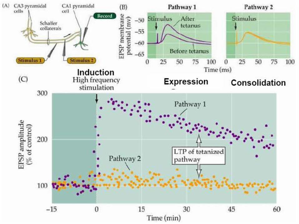
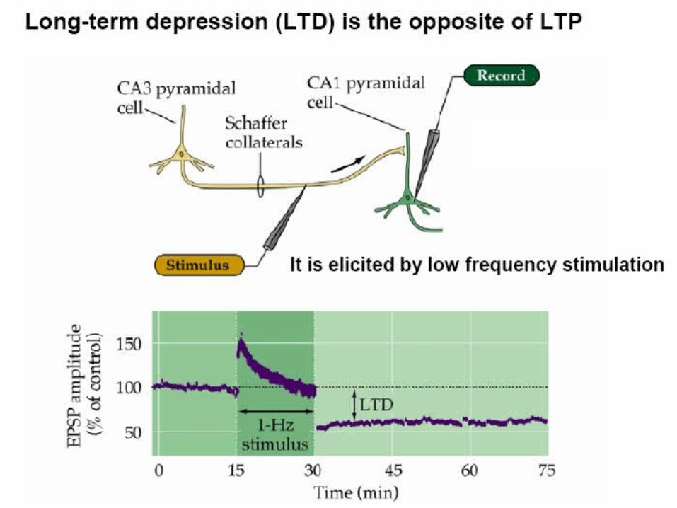
Synaptic plasticity evoked artificially
Examples of Long term potentiation (LTP)and long term depression (LTD).
LTP First demonstrated by Bliss and Lomo in 1973. Since then induced in many different ways, usually in slice.
LTD, robustly shown by Dudek and Bear in 1992, in Hippocampal slice.

17
18

19

20
LTP will lead to new synaptic contacts

21
Conventional LTP = Hebbian Learning
Symmetrical Weight-change curve
Pre
tPre
Post
tPost
Synaptic change %
Pre
tPre
Post
tPost
The temporal order of input and output does not play any role
22

23
Spike timing dependent plasticity - STDP
Markram et. al. 1997

24
Pre follows Post:Long-term Depression
Pre
tPre
Post
tPost
Synaptic
change %
Spike Timing Dependent Plasticity: Temporal Hebbian Learning
Weight-change curve (Bi&Poo, 2001)
Pre
tPre
Post
tPost
Pre precedes Post:Long-term Potentiation
Aca
usal
Causal
(possibly)

25
= v u1 << 1d
dtSingle Input
= v u << 1dw
dtMany Inputs
As v is a single output, it is scalar.
Averaging Inputs= <v u> << 1
dw
dt
We can just average over all input patterns and approximate the weight change by this. Remember, this assumes that weight changes are slow.
If we replace v with w . u we can write:
= Q . w where Q = <uu> is the input correlation matrix
dw
dt
Note: Hebb yields an instable (always growing) weight vector!
Back to the Math. We had:

26
= (v - ) u << 1dw
dt
Covariance Rule(s)
Normally firing rates are only positive and plain Hebb would yield only LTP.Hence we introduce a threshold to also get LTD
Output threshold
= v (u - << 1dw
dtInput vector threshold
Many times one sets the threshold as the average activity of somereference time period (training period)
= <v> or = <u> together with v = w . u we get:
= C . w, where C is the covariance matrix of the input
dw
dthttp://en.wikipedia.org/wiki/Covariance_matrix
C = <(u-<u>)(u-<u>)> = <uu> - <u2> = <(u-<u>)u>

27
The covariance rule can produce LTP without (!) post-synaptic output.This is biologically unrealistic and the BCM rule (Bienenstock, Cooper,Munro) takes care of this.
BCM- Rule
= vu (v - ) << 1dw
dt
As such this rule is again unstable, but BCM introduces a sliding threshold
= (v2 - ) < 1d
dt
Note the rate of threshold change should be faster than then weight
changes (), but slower than the presentation of the individual inputpatterns. This way the weight growth will be over-dampened relative to the (weight – induced) activity increase.

28
Evidence for weight normalization:Reduced weight increase as soon as weights are already big(Bi and Poo, 1998, J. Neurosci.)
Problem: Hebbian Learning can lead to unlimited weight growth.
Solution: Weight normalizationa) subtractive (subtract the mean change of all weights from each individual weight).b) multiplicative (mult. each weight by a gradually decreasing factor).
29
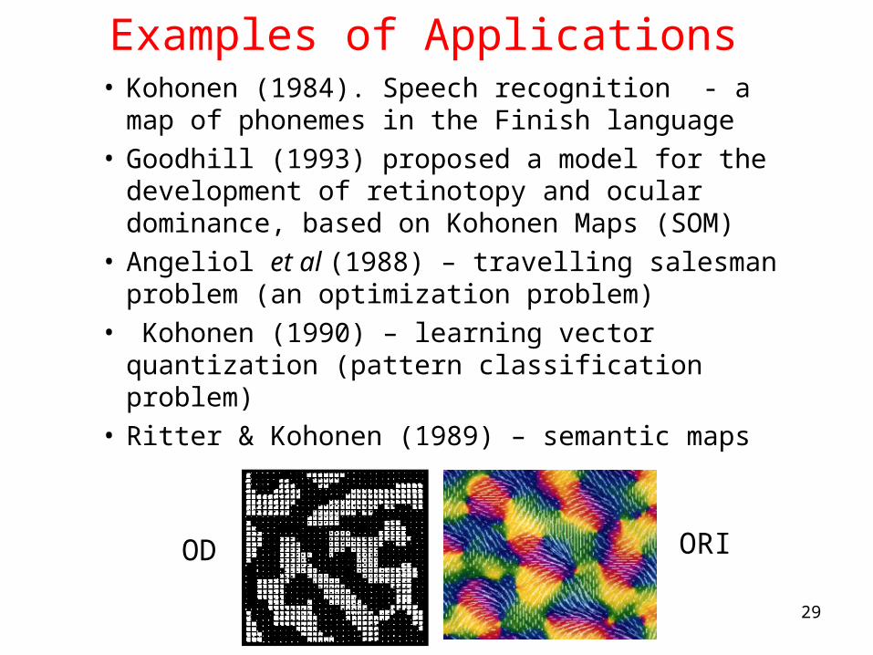
Examples of Applications • Kohonen (1984). Speech recognition - a map of
phonemes in the Finish language• Goodhill (1993) proposed a model for the
development of retinotopy and ocular dominance, based on Kohonen Maps (SOM)
• Angeliol et al (1988) – travelling salesman problem (an optimization problem)
• Kohonen (1990) – learning vector quantization (pattern classification problem)
• Ritter & Kohonen (1989) – semantic maps
OD ORI
30
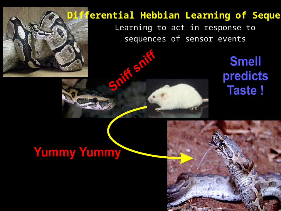
Differential Hebbian Learning of SequencesLearning to act in response to
sequences of sensor events
31
Machine Learning Classical Conditioning Synaptic Plasticity
Dynamic Prog.(Bellman Eq.)
REINFORCEMENT LEARNING UN-SUPERVISED LEARNINGexample based correlation based
d-Rule
Monte CarloControl
Q-Learning
TD( )often =0
ll
TD(1) TD(0)
Rescorla/Wagner
Neur.TD-Models(“Critic”)
Neur.TD-formalism
DifferentialHebb-Rule
(”fast”)
STDP-Modelsbiophysical & network
EVALUATIVE FEEDBACK (Rewards)
NON-EVALUATIVE FEEDBACK (Correlations)
SARSA
Correlationbased Control
(non-evaluative)
ISO-Learning
ISO-Modelof STDP
Actor/Critictechnical & Basal Gangl.
Eligibility Traces
Hebb-Rule
DifferentialHebb-Rule
(”slow”)
supervised L.
Anticipatory Control of Actions and Prediction of Values Correlation of Signals
=
=
=
Neuronal Reward Systems(Basal Ganglia)
Biophys. of Syn. PlasticityDopamine Glutamate
STDP
LTP(LTD=anti)
ISO-Control
Overview over different methods
You are here !

32
I. Pawlow
History of the Concept of TemporallyAsymmetrical Learning: Classical Conditioning
33

34
I. Pawlow
History of the Concept of TemporallyAsymmetrical Learning: Classical Conditioning
Correlating two stimuli which are shifted with respect to each other in time.
Pavlov’s Dog: “Bell comes earlier than Food”
This requires to remember the stimuli in the system.
Eligibility Trace: A synapse remains “eligible” for modification for some time after it was active (Hull 1938, then a still abstract concept).

35
0 = 1
1
Unconditioned Stimulus (Food)
Conditioned Stimulus (Bell)
Response
X
+Stimulus Trace E
The first stimulus needs to be “remembered” in the system
Classical Conditioning: Eligibility Traces

36
I. Pawlow
History of the Concept of TemporallyAsymmetrical Learning: Classical Conditioning
Eligibility Traces
Note: There are vastly different time-scales for (Pavlov’s) hehavioural experiments:
Typically up to 4 seconds
as compared to STDP at neurons:
Typically 40-60 milliseconds (max.)
37
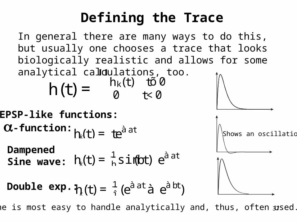
Defining the TraceIn general there are many ways to do this, but usually one chooses a trace that looks biologically realistic and allows for some analytical calculations, too.
EPSP-like functions:-function:
Double exp.:
This one is most easy to handle analytically and, thus, often used.
DampenedSine wave:
Shows an oscillation.
h(t) =n
0 t<0hk(t) tõ 0
h(t) = teà atk
h(t) = b1sin(bt) eà at
k
h(t) = î1(eà at à eà bt)
k

38
Machine Learning Classical Conditioning Synaptic Plasticity
Dynamic Prog.(Bellman Eq.)
REINFORCEMENT LEARNING UN-SUPERVISED LEARNINGexample based correlation based
d-Rule
Monte CarloControl
Q-Learning
TD( )often =0
ll
TD(1) TD(0)
Rescorla/Wagner
Neur.TD-Models(“Critic”)
Neur.TD-formalism
DifferentialHebb-Rule
(”fast”)
STDP-Modelsbiophysical & network
EVALUATIVE FEEDBACK (Rewards)
NON-EVALUATIVE FEEDBACK (Correlations)
SARSA
Correlationbased Control
(non-evaluative)
ISO-Learning
ISO-Modelof STDP
Actor/Critictechnical & Basal Gangl.
Eligibility Traces
Hebb-Rule
DifferentialHebb-Rule
(”slow”)
supervised L.
Anticipatory Control of Actions and Prediction of Values Correlation of Signals
=
=
=
Neuronal Reward Systems(Basal Ganglia)
Biophys. of Syn. PlasticityDopamine Glutamate
STDP
LTP(LTD=anti)
ISO-Control
Overview over different methods
Mathematical formulation of learning rules is
similar but time-scales are much different.

39
Early: “Bell”
Late: “Food”
x
)( )( )( tytutdt
dii
Differential Hebb Learning Rule
Xi
X0
Simpler Notationx = Inputu = Traced Input
V
V’(t)
ui
u0

40
Convolution used to define the traced input,
Correlation used to calculate weight growth.
)()()()()()()( xfxgxgxfduuxgufxh
u
)()()()()()()( xgxfxfxgduxugufxh
w

41
Produces asymmetric weight change curve(if the filters h produce unimodal „humps“)
)(' )( )( tvtutdt
dii
Derivative of the Output
Filtered Input
)( )()( tuttv ii
Output
T
Differential Hebbian Learning

42
Conventional LTP
Symmetrical Weight-change curve
Pre
tPre
Post
tPost
Synaptic change %
Pre
tPre
Post
tPost
The temporal order of input and output does not play any role

43
Produces asymmetric weight change curve(if the filters h produce unimodal „humps“)
)(' )( )( tvtutdt
dii
Derivative of the Output
Filtered Input
)( )()( tuttv ii
Output
T
Differential Hebbian Learning

44Weight-change curve
(Bi&Poo, 2001)
T=tPost - tPrems
Pre follows Post:Long-term Depression
Pre
tPre
Post
tPost
Synaptic change %Pre
tPre
Post
tPost
Pre precedes Post:Long-term Potentiation
Spike-timing-dependent plasticity(STDP): Some vague shape similarity

45
Machine Learning Classical Conditioning Synaptic Plasticity
Dynamic Prog.(Bellman Eq.)
REINFORCEMENT LEARNING UN-SUPERVISED LEARNINGexample based correlation based
d-Rule
Monte CarloControl
Q-Learning
TD( )often =0
ll
TD(1) TD(0)
Rescorla/Wagner
Neur.TD-Models(“Critic”)
Neur.TD-formalism
DifferentialHebb-Rule
(”fast”)
STDP-Modelsbiophysical & network
EVALUATIVE FEEDBACK (Rewards)
NON-EVALUATIVE FEEDBACK (Correlations)
SARSA
Correlationbased Control
(non-evaluative)
ISO-Learning
ISO-Modelof STDP
Actor/Critictechnical & Basal Gangl.
Eligibility Traces
Hebb-Rule
DifferentialHebb-Rule
(”slow”)
supervised L.
Anticipatory Control of Actions and Prediction of Values Correlation of Signals
=
=
=
Neuronal Reward Systems(Basal Ganglia)
Biophys. of Syn. PlasticityDopamine Glutamate
STDP
LTP(LTD=anti)
ISO-Control
Overview over different methods
You are here !

46
PlasticSynapse
NMDA/AMPA
Postsynaptic:Source of Depolarization
The biophysical equivalent of Hebb’s postulate
Presynaptic Signal(Glu)
Pre-Post Correlation,but why is this needed?

47
i n
o u t
i n
o u t
Plasticity is mainly mediated by so calledN-methyl-D-Aspartate (NMDA) channels.
These channels respond to Glutamate as their transmitter andthey are voltage depended:
48
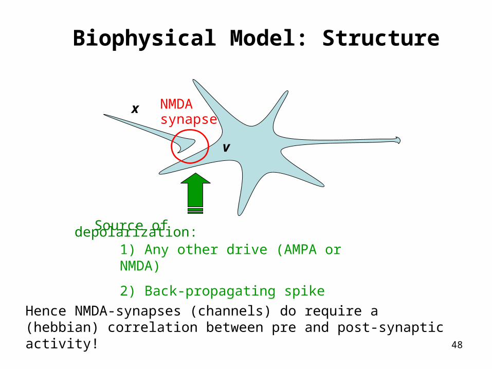
Biophysical Model: Structure
x NMDA synapse
v
Hence NMDA-synapses (channels) do require a (hebbian) correlation between pre and post-synaptic activity!
Source of depolarization:
1) Any other drive (AMPA or NMDA)
2) Back-propagating spike

49
Local Events at the Synapse
Local
Current sources “under” the synapse:• Synaptic current
Isynaptic
GlobalIBP
• Influence of a Back-propagating spike
• Currents from all parts of the dendritic tree
IDendritic
u1
x1
v

51
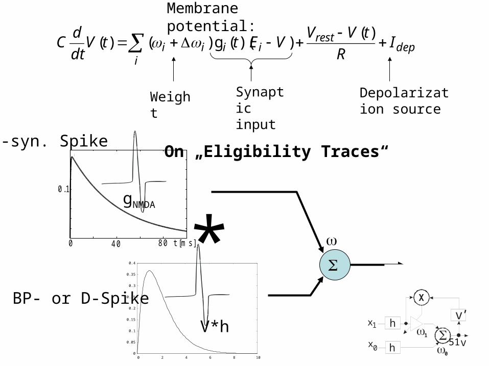
Pre-syn. Spike
BP- or D-Spike
* 0
0.05
0.1
0.15
0.2
0.25
0.3
0.35
0.4
0 2 4 6 8 10
V*h
gNMDA
0 40 80 t [ms]
g [nS ]NM DA
0.1
On „Eligibility Traces“
Membrane potential:
Weight Synaptic input
Depolarization source
deprest
iii
ii IR
tVVVEttV
dt
dC
)(
))((g )()(
1
0
X
v
v’
ISO-Learning
h
h
x
x0
1

52
• Dendritic compartment
• Plastic synapse with NMDA channels Source of Ca2+ influx and coincidence detector
PlasticSynapse NMDA/AMPA
depi
ii IVEt~dt
dV ))((g
NMDA/AMPAgBP spike
Source of Depolarization
Dendritic spike
• Source of depolarization: 1. Back-propagating spike 2. Local dendritic spike
Model structure
53
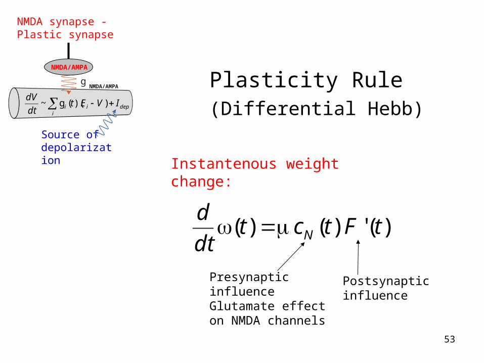
Plasticity Rule(Differential Hebb)
NMDA synapse -Plastic synapse
depi
ii IVEtdt
dV ))((g ~
NMDA/AMPAg
NMDA/AMPA
Source of depolarization
Instantenous weight change:
)(' )( )( tFtctdt
dN
Presynaptic influence Glutamate effect on NMDA channels
Postsynaptic influence

54
0 40 80 t [ms]
g [nS ]NM DA
0.1
Normalized NMDA conductance:
NMDA channels are instrumental for LTP and LTD induction (Malenka and Nicoll, 1999; Dudek and Bear ,1992)
V
tt
N eMg
eec
][1 2
// 21
Pre-synaptic influence
NMDA synapse -Plastic synapse
depi
ii IVEtdt
dV ))((g ~
NMDA/AMPAg
NMDA/AMPA
Source of depolarization
)(' )( )( tFtctdt
dN

55
0 10
0
-40
-60
-20
20V [m V]
20 t [m s]
0 10
0
-40
-60
-20
20V [m V]
20 t [ms]
0 10
0
-40
-60
-20
20V [m V]
20 t [m s]
0 10
0
-40
-60
-20
20V [m V]
20 t [m s]
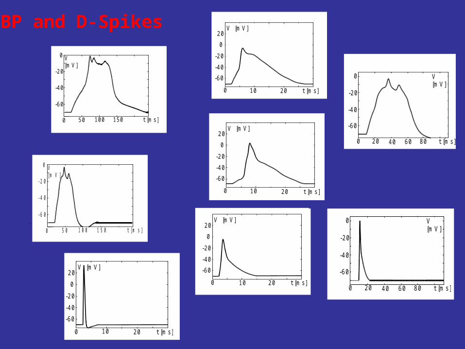
Dendriticspikes
Back-propagating spikes
(Larkum et al., 2001
Golding et al, 2002
Häusser and Mel, 2003)
(Stuart et al., 1997)
Depolarizing potentials in the dendritic tree
56
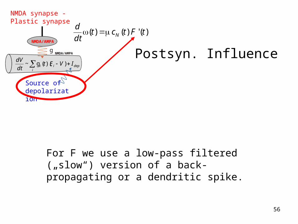
NMDA synapse -Plastic synapse
depi
ii IVEtdt
dV ))((g ~
NMDA/AMPAg
NMDA/AMPA
Source of depolarization
Postsyn. Influence
)(' )( )( tFtctdt
dN
For F we use a low-pass filtered („slow“) version of a back-propagating or a dendritic spike.
57
0 10
0
-40
-60
-20
20V [m V]
20 t [m s]
0 10
0
-40
-60
-20
20V [m V]
20 t [m s]
0 50 150 t [ms]100
0
-40
-60
-20
V [mV]
0 5 0 1 5 0 t [ m s ]1 0 0
0
- 4 0
- 6 0
- 2 0
V [ m V ]
0 20 80 t [ms]40 60
0
-40
-60
-20
V [mV]
0 20 80 t [ms]40 60
0
-40
-60
-20
V [mV]
0 10
0
-40
-60
-20
20V [m V]
20 t [ms]
0 10
0
-40
-60
-20
20V [m V]
20 t [m s]
BP and D-Spikes

58
0 10
0
-40
-60
-20
20V [m V]
20 t [m s]
0 10
0
-40
-60
-20
20V [m V]
20 t [m s]
0-20 40 T [ms]-40 20
-0.01
-0.03
-0.01
0.01
0-20 40 T [ms]-40 20
-0.01
-0.03
-0.01
0.01
Back-propagating spike
Weight change curve
T
NMDAr activation
Back-propagating spike
T=tPost – tPre
Weight Change Curves
Source of Depolarization: Back-Propagating Spikes
59
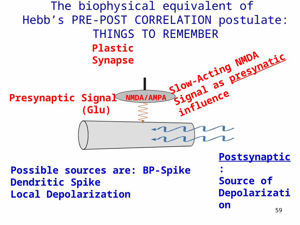
PlasticSynapse
NMDA/AMPA
Postsynaptic:Source of Depolarization
The biophysical equivalent of Hebb’s PRE-POST CORRELATION postulate:
THINGS TO REMEMBER
Presynaptic Signal(Glu)
Possible sources are: BP-SpikeDendritic SpikeLocal Depolarization
Slow-Acting NMDA
Signal as presynatic
influence

60
One word about
Supervised Learning

61
Machine Learning Classical Conditioning Synaptic Plasticity
Dynamic Prog.(Bellman Eq.)
REINFORCEMENT LEARNING UN-SUPERVISED LEARNINGexample based correlation based
d-Rule
Monte CarloControl
Q-Learning
TD( )often =0
ll
TD(1) TD(0)
Rescorla/Wagner
Neur.TD-Models(“Critic”)
Neur.TD-formalism
DifferentialHebb-Rule
(”fast”)
STDP-Modelsbiophysical & network
EVALUATIVE FEEDBACK (Rewards)
NON-EVALUATIVE FEEDBACK (Correlations)
SARSA
Correlationbased Control
(non-evaluative)
ISO-Learning
ISO-Modelof STDP
Actor/Critictechnical & Basal Gangl.
Eligibility Traces
Hebb-Rule
DifferentialHebb-Rule
(”slow”)
supervised L.
Anticipatory Control of Actions and Prediction of Values Correlation of Signals
=
=
=
Neuronal Reward Systems(Basal Ganglia)
Biophys. of Syn. PlasticityDopamine Glutamate
STDP
LTP(LTD=anti)
ISO-Control
Overview over different methods – Supervised Learning
You are
her
e !
And many more

62
Supervised learningmethods are mostlynon-neuronal andwill therefore not
be discussedhere.

63
So Far:
• Open Loop Learning
All slides so far !

64
CLOSED LOOP LEARNING
• Learning to Act (to produce appropriate behavior)
• Instrumental (Operant) Conditioning
All slides to come now !

65
This is an open-loopsystem
Sensor 2
conditionedInput
Bell Food Salivation
Pavlov, 1927
Temporal Sequence
This is an Open Loop System !
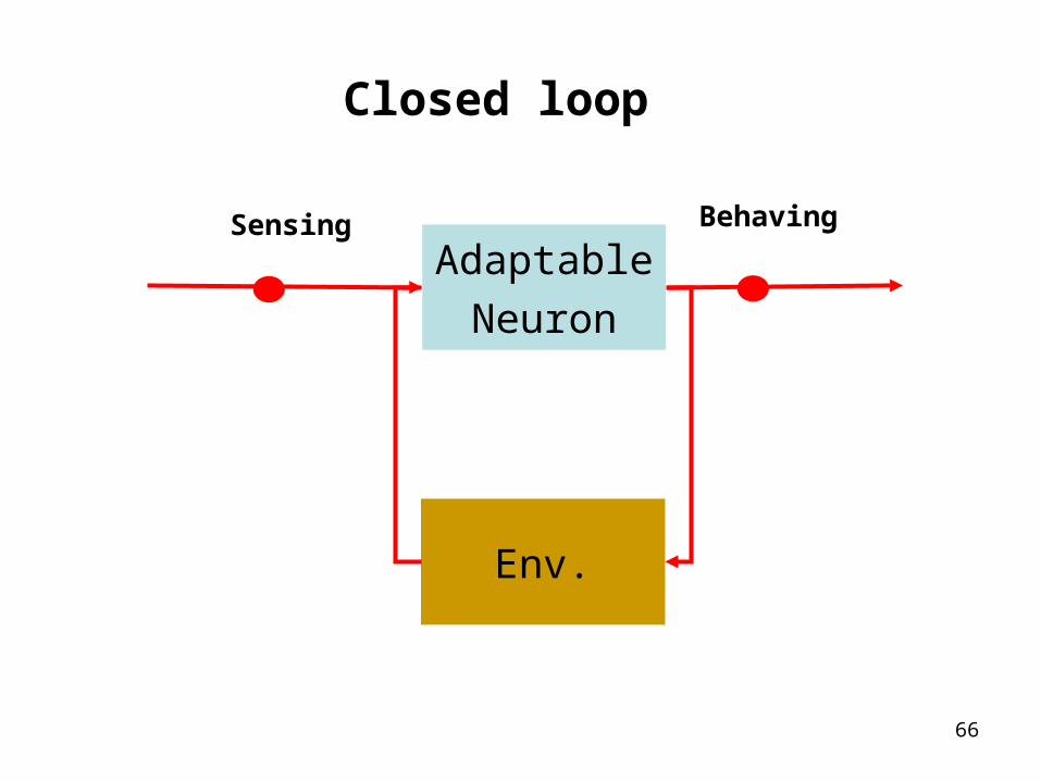
66
Adaptable
Neuron
Env.
Closed loop
Sensing Behaving

67
Instrumental/Operant Conditioning

68
Machine Learning Classical Conditioning Synaptic Plasticity
Dynamic Prog.(Bellman Eq.)
REINFORCEMENT LEARNING UN-SUPERVISED LEARNINGexample based correlation based
d-Rule
Monte CarloControl
Q-Learning
TD( )often =0
ll
TD(1) TD(0)
Rescorla/Wagner
Neur.TD-Models(“Critic”)
Neur.TD-formalism
DifferentialHebb-Rule
(”fast”)
STDP-Modelsbiophysical & network
EVALUATIVE FEEDBACK (Rewards)
NON-EVALUATIVE FEEDBACK (Correlations)
SARSA
Correlationbased Control
(non-evaluative)
ISO-Learning
ISO-Modelof STDP
Actor/Critictechnical & Basal Gangl.
Eligibility Traces
Hebb-Rule
DifferentialHebb-Rule
(”slow”)
supervised L.
Anticipatory Control of Actions and Prediction of Values Correlation of Signals
=
=
=
Neuronal Reward Systems(Basal Ganglia)
Biophys. of Syn. PlasticityDopamine Glutamate
STDP
LTP(LTD=anti)
ISO-Control
Overview over different methods – Closed Loop Learning

69
Behaviorism“All we need to know in order
to describe and explain behavior is this: actions
followed by good outcomes are likely to recur, and actions followed by bad
outcomes are less likely to recur.” (Skinner, 1953)
Skinner had invented the type of experiments called operant conditioning.
B.F. Skinner (1904-1990)
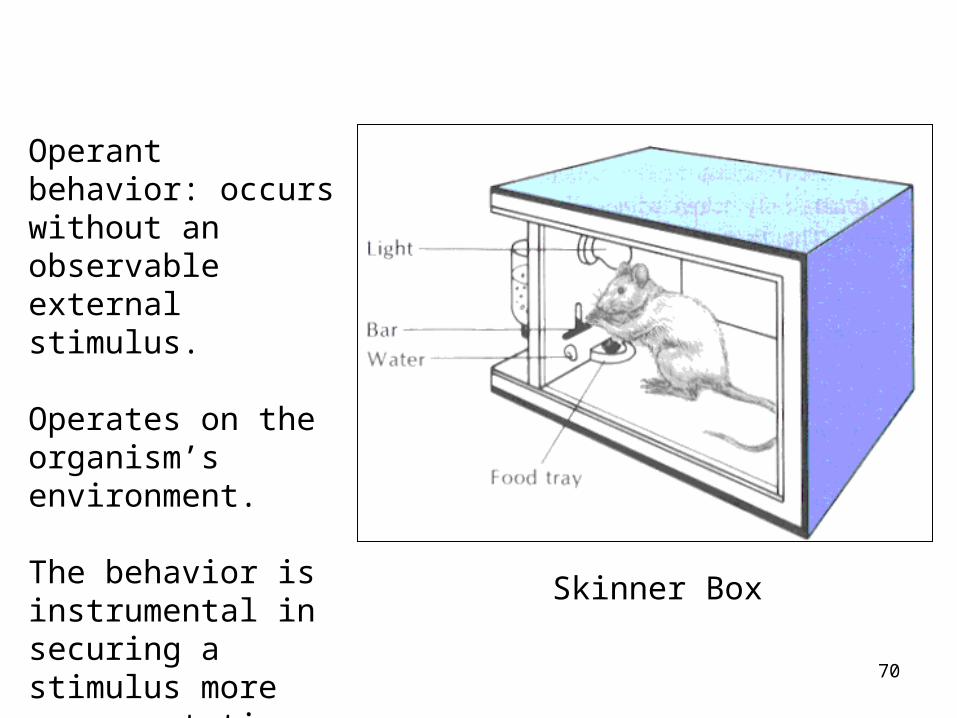
70
Operant behavior: occurs without an observable external stimulus. Operates on the organism’s environment. The behavior is instrumental in securing a stimulus more representative of everyday learning.
Skinner Box

71
OPERANT CONDITIONING TECHNIQUES
• POSITIVE REINFORCEMENT = increasing a behavior by administering a reward
• NEGATIVE REINFORCEMENT = increasing a behavior by removing an aversive stimulus when a behavior occurs
• PUNISHMENT = decreasing a behavior by administering an aversive stimulus following a behavior OR by removing a positive stimulus
• EXTINCTION = decreasing a behavior by not rewarding it

72
Machine Learning Classical Conditioning Synaptic Plasticity
Dynamic Prog.(Bellman Eq.)
REINFORCEMENT LEARNING UN-SUPERVISED LEARNINGexample based correlation based
d-Rule
Monte CarloControl
Q-Learning
TD( )often =0
ll
TD(1) TD(0)
Rescorla/Wagner
Neur.TD-Models(“Critic”)
Neur.TD-formalism
DifferentialHebb-Rule
(”fast”)
STDP-Modelsbiophysical & network
EVALUATIVE FEEDBACK (Rewards)
NON-EVALUATIVE FEEDBACK (Correlations)
SARSA
Correlationbased Control
(non-evaluative)
ISO-Learning
ISO-Modelof STDP
Actor/Critictechnical & Basal Gangl.
Eligibility Traces
Hebb-Rule
DifferentialHebb-Rule
(”slow”)
supervised L.
Anticipatory Control of Actions and Prediction of Values Correlation of Signals
=
=
=
Neuronal Reward Systems(Basal Ganglia)
Biophys. of Syn. PlasticityDopamine Glutamate
STDP
LTP(LTD=anti)
ISO-Control
Overview over different methods
You are here !
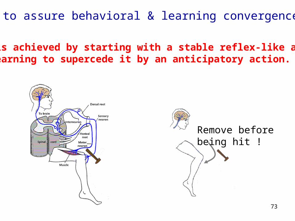
73
How to assure behavioral & learning convergence ??
This is achieved by starting with a stable reflex-like actionand learning to supercede it by an anticipatory action.
Remove beforebeing hit !

74
C o n tro lle rC o n tro lled
S ystemC o n tro lS ign a ls
F e edb ack
D is tu rba ncesS e t-P o in t
X 0
Reflex Only
(Compare to an electronic closed loop controller!)
This structure assures initial (behavioral) stability (“homeostasis”)
Think of a Thermostat !

75
Robot Application
x
Early: “Vision”
Late: “Bump”

76
Robot Application
Initially built-in behavior: Retraction reaction whenever an obstacle is touched.
Learning Goal:Correlate the vision signals with the touch signals and navigate without collisions.

77
Robot Example

78
ControllerControlled
SystemControlSignals
Feedback
DisturbancesSet-Point
X0X1early late
What has happened during learningto the system ?
The primary reflex re-action has effectively been eliminatedand replaced by an anticipatory action

Reinforcement Learning (RL)
Learning from rewards (and punishments)
Learning to assess the value of states.
Learning goal directed behavior.
RL has been developed rather independently from two different fields:
1) Dynamic Programming and Machine Learning (Bellman Equation).
2) Psychology (Classical Conditioning) and later Neuroscience (Dopamine System in the brain)

I. Pawlow
Back to Classical Conditioning
U(C)S = Unconditioned Stimulus
U(C)R = Unconditioned Response
CS = Conditioned Stimulus
CR = Conditioned Response

Less “classical” but also Conditioning !(Example from a car advertisement)
Learning the association
CS → U(C)RPorsche → Good Feeling

Machine Learning Classical Conditioning Synaptic Plasticity
Dynamic Prog.(Bellman Eq.)
REINFORCEMENT LEARNING UN-SUPERVISED LEARNINGexample based correlation based
d-Rule
Monte CarloControl
Q-Learning
TD( )often =0
ll
TD(1) TD(0)
Rescorla/Wagner
Neur.TD-Models(“Critic”)
Neur.TD-formalism
DifferentialHebb-Rule
(”fast”)
STDP-Modelsbiophysical & network
EVALUATIVE FEEDBACK (Rewards)
NON-EVALUATIVE FEEDBACK (Correlations)
SARSA
Correlationbased Control
(non-evaluative)
ISO-Learning
ISO-Modelof STDP
Actor/Critictechnical & Basal Gangl.
Eligibility Traces
Hebb-Rule
DifferentialHebb-Rule
(”slow”)
supervised L.
Anticipatory Control of Actions and Prediction of Values Correlation of Signals
=
=
=
Neuronal Reward Systems(Basal Ganglia)
Biophys. of Syn. PlasticityDopamine Glutamate
STDP
LTP(LTD=anti)
ISO-Control
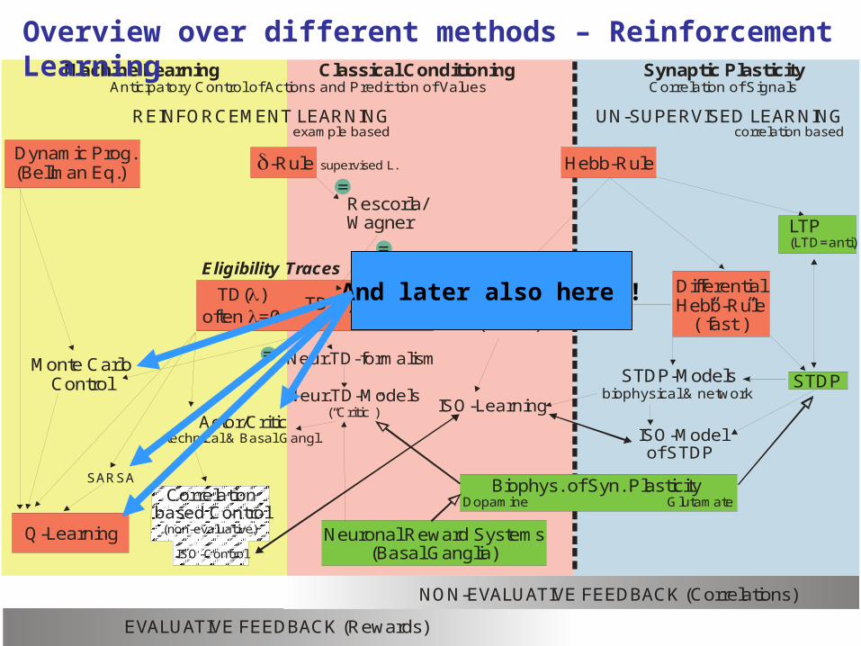
Overview over different methods – Reinforcement Learning
You are here !
Machine Learning Classical Conditioning Synaptic Plasticity
Dynamic Prog.(Bellman Eq.)
REINFORCEMENT LEARNING UN-SUPERVISED LEARNINGexample based correlation based
d-Rule
Monte CarloControl
Q-Learning
TD( )often =0
ll
TD(1) TD(0)
Rescorla/Wagner
Neur.TD-Models(“Critic”)
Neur.TD-formalism
DifferentialHebb-Rule
(”fast”)
STDP-Modelsbiophysical & network
EVALUATIVE FEEDBACK (Rewards)
NON-EVALUATIVE FEEDBACK (Correlations)
SARSA
Correlationbased Control
(non-evaluative)
ISO-Learning
ISO-Modelof STDP
Actor/Critictechnical & Basal Gangl.
Eligibility Traces
Hebb-Rule
DifferentialHebb-Rule
(”slow”)
supervised L.
Anticipatory Control of Actions and Prediction of Values Correlation of Signals
=
=
=
Neuronal Reward Systems(Basal Ganglia)
Biophys. of Syn. PlasticityDopamine Glutamate
STDP
LTP(LTD=anti)
ISO-Control
Overview over different methods – Reinforcement Learning
And later also here !
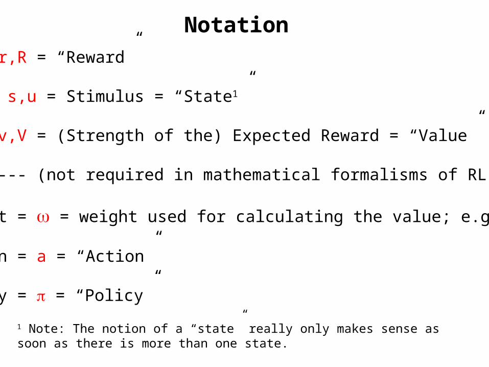
US = r,R = “Reward”
CS = s,u = Stimulus = “State1”
CR = v,V = (Strength of the) Expected Reward = “Value”
UR = --- (not required in mathematical formalisms of RL)
Weight = = weight used for calculating the value; e.g. v=u
Action = a = “Action”
Policy = = “Policy”
1 Note: The notion of a “state” really only makes sense as soon as there is more than one state.
Notation
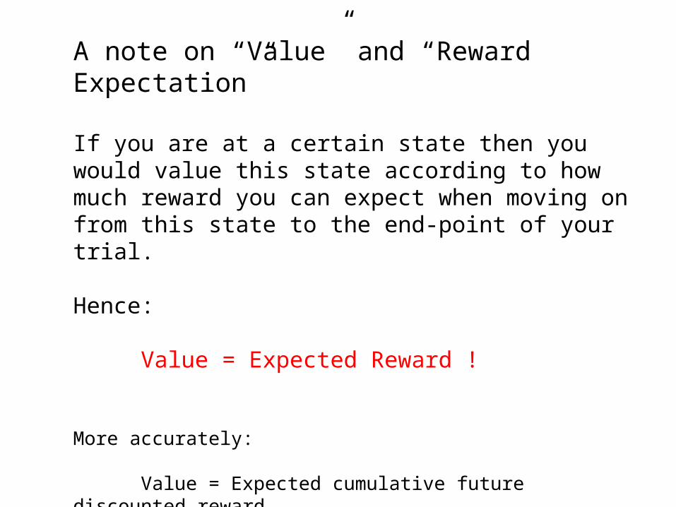
A note on “Value” and “Reward Expectation”
If you are at a certain state then you would value this state according to how much reward you can expect when moving on from this state to the end-point of your trial.
Hence:
Value = Expected Reward !
More accurately:
Value = Expected cumulative future discounted reward.
(for this, see later!)

1) Rescorla-Wagner Rule: Allows for explaining several types of conditioning experiments.
2) TD-rule (TD-algorithm) allows measuring the value of states and allows accumulating rewards. Thereby it generalizes the Resc.-Wagner rule.
3) TD-algorithm can be extended to allow measuring the value of actions and thereby control behavior either by ways of
a) Q or SARSA learning or with
b) Actor-Critic Architectures
Types of Rules

Machine Learning Classical Conditioning Synaptic Plasticity
Dynamic Prog.(Bellman Eq.)
REINFORCEMENT LEARNING UN-SUPERVISED LEARNINGexample based correlation based
d-Rule
Monte CarloControl
Q-Learning
TD( )often =0
ll
TD(1) TD(0)
Rescorla/Wagner
Neur.TD-Models(“Critic”)
Neur.TD-formalism
DifferentialHebb-Rule
(”fast”)
STDP-Modelsbiophysical & network
EVALUATIVE FEEDBACK (Rewards)
NON-EVALUATIVE FEEDBACK (Correlations)
SARSA
Correlationbased Control
(non-evaluative)
ISO-Learning
ISO-Modelof STDP
Actor/Critictechnical & Basal Gangl.
Eligibility Traces
Hebb-Rule
DifferentialHebb-Rule
(”slow”)
supervised L.
Anticipatory Control of Actions and Prediction of Values Correlation of Signals
=
=
=
Neuronal Reward Systems(Basal Ganglia)
Biophys. of Syn. PlasticityDopamine Glutamate
STDP
LTP(LTD=anti)
ISO-Control
Overview over different methods – Reinforcement Learning
You are here !

Rescorla-Wagner Rule
Pavlovian:
Extinction:
Partial:
Train Result
u→r
u→r u→●
Pre-Train
u→r u→●
u→v=max
u→v=0
u→v<max
We define: v = u, with u=1 or u=0, binary and → + du with d = r - v
This learning rule minimizes the avg. squared error between actual reward r and the prediction v, hence min<(r-v)2>
We realize that d is the prediction error.
The associability between stimulus u and reward r is represented by the learning rate .

Extinction10 20 30 40 50 60 70 80 90 100 110 120
-1
-0.8
-0.6
-0.4
-0.2
0
0.2
0.4
0.6
0.8
1
reward expected reward
prediction error
Pawlovian

Pawlovian
Extinction
Partial
Stimulus u is paired with r=1 in 100% of the discrete “epochs” for Pawlovianand in 50% of the cases for Partial.

10 20 30 40 50 60 70 80 90 100 110 120
-1
-0.8
-0.6
-0.4
-0.2
0
0.2
0.4
0.6
0.8
1
Partial (50% reward)

Rescorla-Wagner Rule, Vector Form for Multiple Stimuli
We define: v = w.u, and w → w + du with d = r – v
Where we minimize d
Blocking:
Train Result
u1+u2→r
Pre-Train
u1→v=max, u2→v=0u1→r
For Blocking: The association formed during pre-training leads to d=0. As 2 starts with zero the expected reward v=1u1+2u2 remains at r. This keeps d=0 and the new association with u2 cannot be learned.
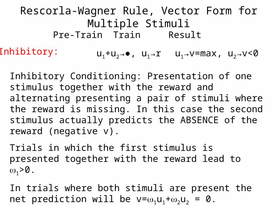
Rescorla-Wagner Rule, Vector Form for Multiple Stimuli
Inhibitory:
Train ResultPre-Train
u1+u2→●, u1→r u1→v=max, u2→v<0
Inhibitory Conditioning: Presentation of one stimulus together with the reward and alternating presenting a pair of stimuli where the reward is missing. In this case the second stimulus actually predicts the ABSENCE of the reward (negative v).
Trials in which the first stimulus is presented together with the reward lead to 1>0.
In trials where both stimuli are present the net prediction will be v=1u1+2u2 = 0.
As u1,2=1 (or zero) and 1>0, we get 2<0 and, consequentially, v(u2)<0.

Rescorla-Wagner Rule, Vector Form for Multiple Stimuli
Overshadow:
Train ResultPre-Train
u1+u2→r u1→v<max, u2→v<max
Overshadowing: Presenting always two stimuli together with the reward will lead to a “sharing” of the reward prediction between them. We get v= 1u1+2u2 = r. Using different learning rates will lead to differently strong growth of 1,2 and represents the often observed different saliency of the two stimuli.

Rescorla-Wagner Rule, Vector Form for Multiple Stimuli
Secondary:
Train ResultPre-Train
u1→r u2→u1 u2→v=max
Secondary Conditioning reflect the “replacement” of one stimulus by a new one for the prediction of a reward.
As we have seen the Rescorla-Wagner Rule is very simple but still able to represent many of the basic findings of diverse conditioning experiments.
Secondary conditioning, however, CANNOT be captured.

Predicting Future Reward
Animals can predict to some degree such sequences and form the correct associations. For this we need algorithms that keep track of time.
Here we do this by ways of states that are subsequently visited and evaluated.
The Rescorla-Wagner Rule cannot deal with the sequentiallity of stimuli (required to deal with Secondary Conditioning). As a consequence it treats this case similar to Inhibitory Conditioning lead to negative 2.

Prediction and Control
The goal of RL is two-fold:
1) To predict the value of states (exploring the state space following a policy) – Prediction Problem.
2) Change the policy towards finding the optimal policy – Control Problem.
• State,• Action,• Reward,• Value,• Policy
Terminology (again):

Markov Decision Problems (MDPs)
1 2 3 4 5 6 7 8
9 10 11 12
13 14
15 16
r1 r2
a2 a15a14a1
s
terminal states
states
actions
rewards
If the future of the system depends always only on the current state and action then the system is said to be “Markovian”.

What does an RL-agent do ?
An RL-agent explores the state space trying to accumulate as much reward as possible. It follows a behavioral policy performing actions (which usually will lead the agent from one state to the next).
For the Prediction Problem: It updates the value of each given state by assessing how much future (!) reward can be obtained when moving onwards from this state (State Space). It does not change the policy, rather it evaluates it. (Policy Evaluation).

For the Control Problem: It updates the value of each given action at a given state and of by assessing how much future reward can be obtained when performing this action at that state (State-Action Space, which is larger
than the State Space). and all following actions at the following state moving onwards.Guess: Will we have to evaluate ALL states and actions onwards?
p(N) = 0.5p(S) = 0.125p(W) = 0.25p(E) = 0.125
Policy:
x x x x x
R R
0.0
value = 0.0everywherereward R=1
possible startlocations
0.9
0.9
0.8
0.1 0.1 0.1 0.1 0.1
etc
Policy Evaluationgive values of states

Exploration – Exploitation Dilemma: The agent wants to get as much cumulative reward (also often called return) as possible. For this it should always perform the most rewarding action “exploiting” its (learned) knowledge of the state space. This way it might however miss an action which leads (a bit further on) to a much more rewarding path. Hence the agent must also “explore” into unknown parts of the state space. The agent must, thus, balance its policy to include exploitation and exploration.
What does an RL-agent do ?
Policies1) Greedy Policy: The agent always exploits and
selects the most rewarding action. This is sub-optimal as the agent never finds better new paths.

Policies2 -Greedy Policy: With a small probability the
agent will choose a non-optimal action. *All non-optimal actions are chosen with equal probability.* This can take very long as it is not known how big should be. One can also “anneal” the system by gradually lowering to become more and more greedy.
3) Softmax Policy: -greedy can be problematic because of (*). Softmax ranks the actions according to their values and chooses roughly following the ranking using for example:
P
b=1
n
exp( TQb)
exp( TQa) where Qa is value of the
currently to be evaluated action a and T is a temperature parameter. For large T all actions have approx. equal probability to get selected.

Machine Learning Classical Conditioning Synaptic Plasticity
Dynamic Prog.(Bellman Eq.)
REINFORCEMENT LEARNING UN-SUPERVISED LEARNINGexample based correlation based
d-Rule
Monte CarloControl
Q-Learning
TD( )often =0
ll
TD(1) TD(0)
Rescorla/Wagner
Neur.TD-Models(“Critic”)
Neur.TD-formalism
DifferentialHebb-Rule
(”fast”)
STDP-Modelsbiophysical & network
EVALUATIVE FEEDBACK (Rewards)
NON-EVALUATIVE FEEDBACK (Correlations)
SARSA
Correlationbased Control
(non-evaluative)
ISO-Learning
ISO-Modelof STDP
Actor/Critictechnical & Basal Gangl.
Eligibility Traces
Hebb-Rule
DifferentialHebb-Rule
(”slow”)
supervised L.
Anticipatory Control of Actions and Prediction of Values Correlation of Signals
=
=
=
Neuronal Reward Systems(Basal Ganglia)
Biophys. of Syn. PlasticityDopamine Glutamate
STDP
LTP(LTD=anti)
ISO-Control
Overview over different methods – Reinforcement Learning
You are here !
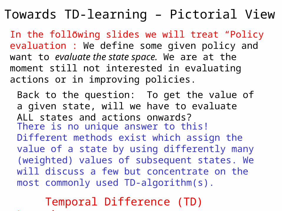
Back to the question: To get the value of a given state, will we have to evaluate ALL states and actions onwards?There is no unique answer to this! Different methods exist which assign the value of a state by using differently many (weighted) values of subsequent states. We will discuss a few but concentrate on the most commonly used TD-algorithm(s).
Temporal Difference (TD) Learning
Towards TD-learning – Pictorial View
In the following slides we will treat “Policy evaluation”: We define some given policy and want to evaluate the state space. We are at the moment still not interested in evaluating actions or in improving policies.

Formalising RL: Policy Evaluation with goal to find the optimal value function of the state spaceWe consider a sequence st, rt+1, st+1, rt+2, . . . , rT , sT . Note, rewards occur downstream (in the future) from a visited state. Thus, rt+1 is the next future reward which can be reached starting from state st. The complete return Rt to be expected in the future from state st is, thus, given by:
where ≤1 is a discount factor. This accounts for the fact that rewards in the far future should be valued less.Reinforcement learning assumes that the value of a state V(s) is directly equivalent to the expected return E at this state, where denotes the (here unspecified) action policy to be followed.
Thus, the value of state st can be iteratively updated with:

We use as a step-size parameter, which is not of great importance here, though, and can be held constant.Note, if V(st) correctly predicts the expected complete return Rt, the update will be zero and we have found the final value. This method is called constant- Monte Carlo update. It requires to wait until a sequence has reached its terminal state (see some slides before!) before the update can commence. For long sequences this may be problematic. Thus, one should try to use an incremental procedure instead. We define a different update rule with:
The elegant trick is to assume that, if the process converges, the value of the next state V(st+1) should be an accurate estimate of the expected return downstream to this state (i.e., downstream to st+1). Thus, we would hope that the following holds:Indeed, proofs exist that under certain boundary conditions this procedure, known as TD(0), converges to the optimal value function for all states.
This is why it is called TD (temp. diff.) Learning
| {z }
Machine Learning Classical Conditioning Synaptic Plasticity
Dynamic Prog.(Bellman Eq.)
REINFORCEMENT LEARNING UN-SUPERVISED LEARNINGexample based correlation based
d-Rule
Monte CarloControl
Q-Learning
TD( )often =0
ll
TD(1) TD(0)
Rescorla/Wagner
Neur.TD-Models(“Critic”)
Neur.TD-formalism
DifferentialHebb-Rule
(”fast”)
STDP-Modelsbiophysical & network
EVALUATIVE FEEDBACK (Rewards)
NON-EVALUATIVE FEEDBACK (Correlations)
SARSA
Correlationbased Control
(non-evaluative)
ISO-Learning
ISO-Modelof STDP
Actor/Critictechnical & Basal Gangl.
Eligibility Traces
Hebb-Rule
DifferentialHebb-Rule
(”slow”)
supervised L.
Anticipatory Control of Actions and Prediction of Values Correlation of Signals
=
=
=
Neuronal Reward Systems(Basal Ganglia)
Biophys. of Syn. PlasticityDopamine Glutamate
STDP
LTP(LTD=anti)
ISO-Control
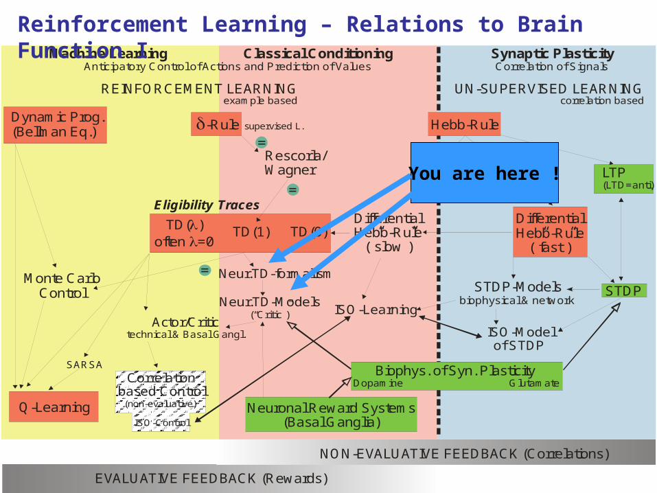
Reinforcement Learning – Relations to Brain Function I
You are here !

Trace
d
1
X
x1
r
vv’
E
u1
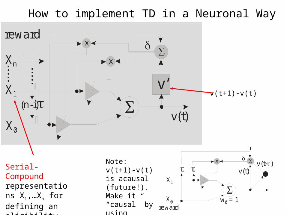
How to implement TD in a Neuronal Way
Now we have:
wi ! wi + ö[r(t + 1) + í v(t + 1) à v(t)]uà(t)
We had defined:(first lecture!)
X0
X1
Xn
v(t)
x
x
v’
reward
(n-i)
d
How to implement TD in a Neuronal Way
v(t+1)-v(t)
Note: v(t+1)-v(t) is acausal (future!). Make it “causal” by using delays.
x
w = 10X0
X1
reward
d
v(t)v(t- )
r
Serial-Compound representations X1,…Xn for defining an eligibility trace.
Machine Learning Classical Conditioning Synaptic Plasticity
Dynamic Prog.(Bellman Eq.)
REINFORCEMENT LEARNING UN-SUPERVISED LEARNINGexample based correlation based
d-Rule
Monte CarloControl
Q-Learning
TD( )often =0
ll
TD(1) TD(0)
Rescorla/Wagner
Neur.TD-Models(“Critic”)
Neur.TD-formalism
DifferentialHebb-Rule
(”fast”)
STDP-Modelsbiophysical & network
EVALUATIVE FEEDBACK (Rewards)
NON-EVALUATIVE FEEDBACK (Correlations)
SARSA
Correlationbased Control
(non-evaluative)
ISO-Learning
ISO-Modelof STDP
Actor/Critictechnical & Basal Gangl.
Eligibility Traces
Hebb-Rule
DifferentialHebb-Rule
(”slow”)
supervised L.
Anticipatory Control of Actions and Prediction of Values Correlation of Signals
=
=
=
Neuronal Reward Systems(Basal Ganglia)
Biophys. of Syn. PlasticityDopamine Glutamate
STDP
LTP(LTD=anti)
ISO-Control
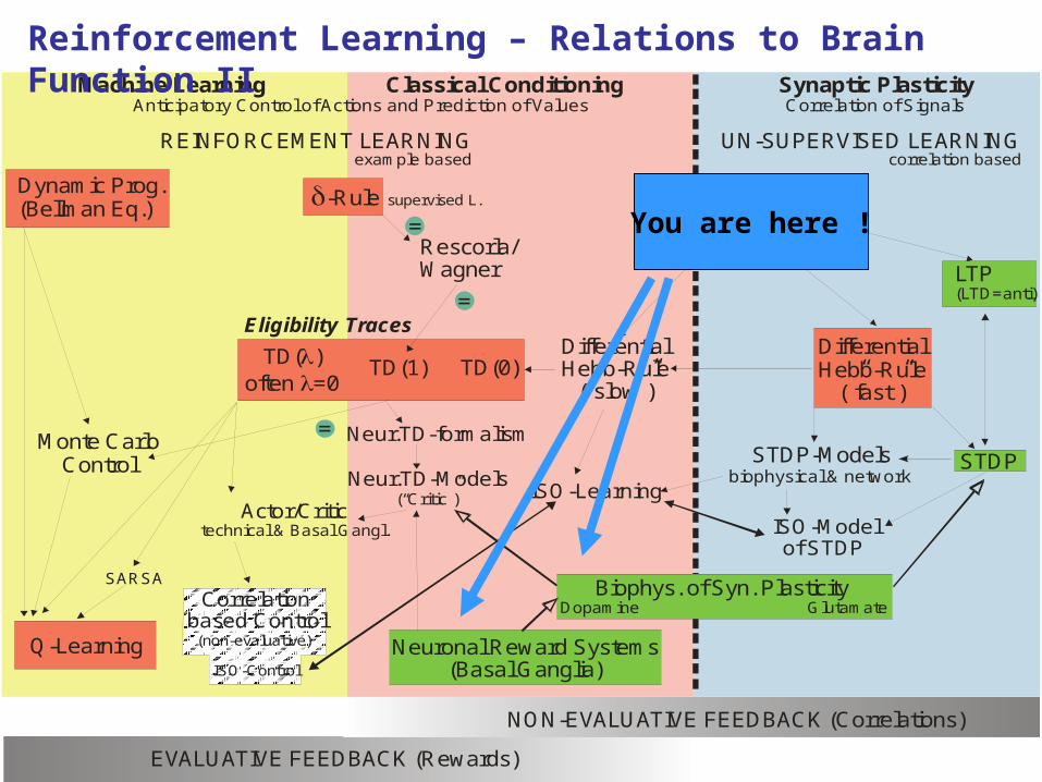
Reinforcement Learning – Relations to Brain Function II
You are here !

TD-learning & Brain FunctionNovelty Response:no prediction,reward occurs
no CS r
After learning:predicted reward occurs
CS r
DA-responses in the basal ganglia pars compacta of thesubstantia nigra and the medially adjoining ventral tegmental area (VTA).
This neuron is supposed to represent the d-error of TD-learning, which has moved forward as expected.
After learning:predicted reward does notoccur
CS 1.0 s
Omission of reward leads to inhibition as also predicted by the TD-rule.

TD-learning & Brain Function
1.5 srTr
RewardExpectation
This neuron is supposed to represent the reward expectation signal v. It has extended forward (almost) to the CS (here called Tr) as expected from the TD-rule. Such neurons are found in the striatum, orbitofrontal cortex and amygdala.
1.0 s
Reward Expectation(Population Response)
Tr r
This is even better visible from the population response of 68 striatal neurons
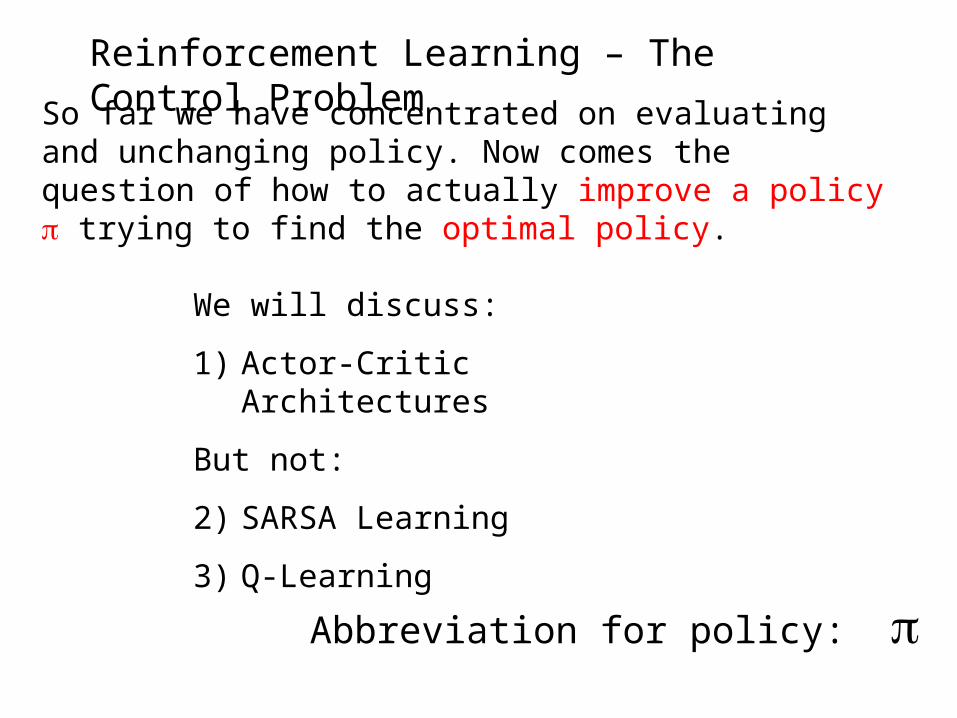
Reinforcement Learning – The Control ProblemSo far we have concentrated on evaluating and
unchanging policy. Now comes the question of how to actually improve a policy trying to find the optimal policy.
We will discuss:
1) Actor-Critic Architectures
But not:
2) SARSA Learning
3) Q-Learning
Abbreviation for policy:

Machine Learning Classical Conditioning Synaptic Plasticity
Dynamic Prog.(Bellman Eq.)
REINFORCEMENT LEARNING UN-SUPERVISED LEARNINGexample based correlation based
d-Rule
Monte CarloControl
Q-Learning
TD( )often =0
ll
TD(1) TD(0)
Rescorla/Wagner
Neur.TD-Models(“Critic”)
Neur.TD-formalism
DifferentialHebb-Rule
(”fast”)
STDP-Modelsbiophysical & network
EVALUATIVE FEEDBACK (Rewards)
NON-EVALUATIVE FEEDBACK (Correlations)
SARSA
Correlationbased Control
(non-evaluative)
ISO-Learning
ISO-Modelof STDP
Actor/Critictechnical & Basal Gangl.
Eligibility Traces
Hebb-Rule
DifferentialHebb-Rule
(”slow”)
supervised L.
Anticipatory Control of Actions and Prediction of Values Correlation of Signals
=
=
=
Neuronal Reward Systems(Basal Ganglia)
Biophys. of Syn. PlasticityDopamine Glutamate
STDP
LTP(LTD=anti)
ISO-Control
Reinforcement Learning – Control Problem I
You are here !

Control Loops
ControllerControlled
SystemControlSignals
Feedback
DisturbancesSet-Point
X0
A basic feedback–loop controller (Reflex) as in the slide before.
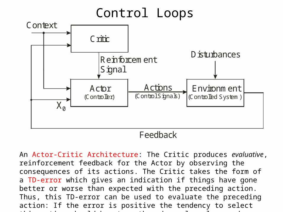
Actor(Controller)
Environment(Controlled System)
Feedback
Disturbances
Context
Critic
Actions(Control Signals)
ReinforcementSignal
X0
Control Loops
An Actor-Critic Architecture: The Critic produces evaluative, reinforcement feedback for the Actor by observing the consequences of its actions. The Critic takes the form of a TD-error which gives an indication if things have gone better or worse than expected with the preceding action. Thus, this TD-error can be used to evaluate the preceding action: If the error is positive the tendency to select this action should be strengthened or else, lessened.

ù(s;a) = Pbep(s;b)
ep(s;a)
Example of an Actor-Critic Procedure
Action selection here follows the Gibb’s Softmax method:
where p(s,a) are the values of the modifiable (by the Critic!) policy parameters of the actor, indicating the tendency to select action a when being in state s.
p(st;at) p(st;at) + ì î t
We can now modify p for a given state action pair at time t with:
where dt is the d-error of the TD-Critic.

Machine Learning Classical Conditioning Synaptic Plasticity
Dynamic Prog.(Bellman Eq.)
REINFORCEMENT LEARNING UN-SUPERVISED LEARNINGexample based correlation based
d-Rule
Monte CarloControl
Q-Learning
TD( )often =0
ll
TD(1) TD(0)
Rescorla/Wagner
Neur.TD-Models(“Critic”)
Neur.TD-formalism
DifferentialHebb-Rule
(”fast”)
STDP-Modelsbiophysical & network
EVALUATIVE FEEDBACK (Rewards)
NON-EVALUATIVE FEEDBACK (Correlations)
SARSA
Correlationbased Control
(non-evaluative)
ISO-Learning
ISO-Modelof STDP
Actor/Critictechnical & Basal Gangl.
Eligibility Traces
Hebb-Rule
DifferentialHebb-Rule
(”slow”)
supervised L.
Anticipatory Control of Actions and Prediction of Values Correlation of Signals
=
=
=
Neuronal Reward Systems(Basal Ganglia)
Biophys. of Syn. PlasticityDopamine Glutamate
STDP
LTP(LTD=anti)
ISO-Control
Reinforcement Learning – Control I & Brain Function III
You are here !
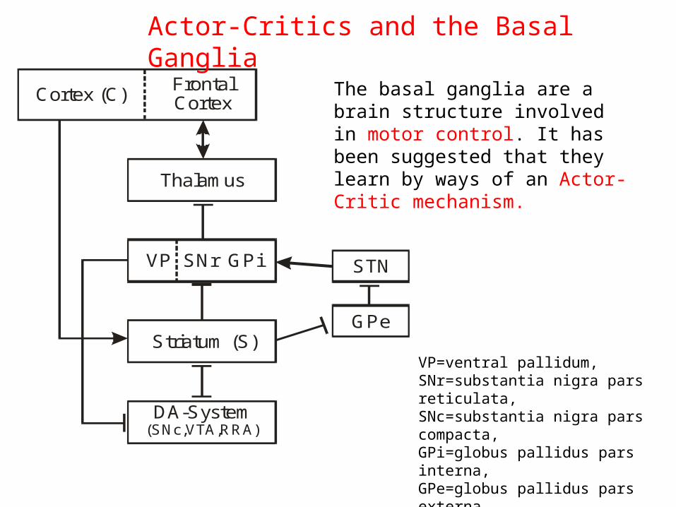
Cortex (C)FrontalCortex
VP SNr GPi
DA-System(SNc,VTA,RRA)
Thalamus
Striatum (S)GPe
STN
Actor-Critics and the Basal Ganglia
VP=ventral pallidum,SNr=substantia nigra pars reticulata,SNc=substantia nigra pars compacta,GPi=globus pallidus pars interna,GPe=globus pallidus pars externa,VTA=ventral tegmental area,RRA=retrorubral area, STN=subthalamic nucleus.
The basal ganglia are a brain structure involved in motor control. It has been suggested that they learn by ways of an Actor-Critic mechanism.

So called striosomal modules of the Striatum S fulfill the functions of the adaptive Critic. The prediction-error (d) characteristics of the DA-neurons of the Critic are generated by: 1) Equating the reward r with excitatory input from the lateral hypothalamus. 2) Equating the term v(t) with indirect excitation at the DA-neurons which is initiated from striatal striosomes and channelled through the subthalamic nucleus onto the DA neurons. 3) Equating the term v(t−1) with direct, long-lasting inhibition from striatal striosomes onto the DA-neurons. There are many problems with this simplistic view though: timing, mismatch to anatomy, etc.
C
S
STN
DA r+
-Cortex=C, striatum=S, STN=subthalamic Nucleus, DA=dopamine system, r=reward.
Actor-Critics and the Basal Ganglia: The Critic
DAGlu
Cortico-striatal(”pre”)
Nigro-striatal(”DA”)
Medium-sized Spiny ProjectionNeuron in the Striatum (”post”)
CDA
d
v(t-1)
v(t)
LH

121
Literature (all of this is very mathematical!)
General Theoretical Neuroscience:
„Theoretical Neuroscience“, P.Dayan and L. Abbott, MIT Press (there used to be a version of this on the internet)
„Spiking Neuron Models“, W. Gerstner & W.M. Kistler, Cambridge University Press. (there is a version on the internet)
Neural Coding Issues: „Spikes“ F. Rieke, D. Warland, R. de Ruyter v. Steveninck, W. Bialek, MIT Press
Artificial Neural Networks: „Konnektionismus“, G. Dorffner, B.G. Teubner Verlg. Stuttgart
„Fundamentals of Artificial Neural Networks“, M.H. Hassoun, MIT Press
Hodgkin Huxley Model: See above „Spiking Neuron Models“, W. Gerstner & W.M. Kistler, Cambridge University Press.
Learning and Plasticity: See above „Spiking Neuron Models“, W. Gerstner & W.M. Kistler, Cambridge University Press.
Calculating with Neurons: Has been compiled from many different sources.
Maps: Has been compiled from many different sources.

122