CS251 Programming Languages Handout # 1Prof. Lyn Turbak December 12, 2017Wellesley College

Hofl, a Higher-order Functional Language

Hofl (Higher Order Functional Language) is a language that extends Valex with first-classfunctions and a recursive binding construct. We study Hofl to understand the design and im-plementation issues involving first-class functions, particularly the notions of static vs. dynamicscoping and recursive binding.

Although Hofl is a “toy” language, it packs a good amount of expressive punch, and could beused for many “real” programming purposes. Indeed, it is very similar to the Racket programminglanguage, and it is powerful enough to write interpreters for all the mini-languages we have studied,including Hofl itself!

In this handout, we introduce the key features of the Hofl language in the context of examples.We also study the implementation of Hofl, particularly with regard to scoping issues.

1 An Overview of Hofl

The Hofl language extends Valex with the following features:

1. Anonymous first-class curried functions and a means of applying these functions;

2. A bindrec form for definining mutually recursive values (typically functions);

3. A load form for loading definitions from files.

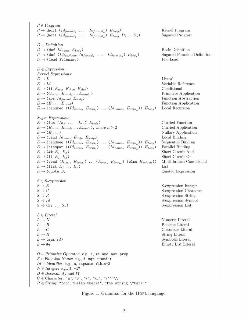
The full grammar of Hofl is presented in figure 1. The syntactic sugar of Hofl is defined infigure 2.

2 Abstractions and Function Applications

In Hofl, anonymous first-class functions are created via

(abs Idformal Ebody )

This denotes a function of a single argument Idformal that computes Ebody . It corresponds to theSML notation fn Idformal => Ebody .

Function application is expressed by the parenthesized notation (Erator Erand), where Erator

is an arbitrary expression that denotes a function, and Erand denotes the operand value to whichthe function is applied. For example:

hofl > ((abs x (* x x)) (+ 1 2))

9

hofl > ((abs f (f 5)) (abs x (* x x)))

25

hofl > ((abs f (f 5)) ((abs x (abs y (+ x y))) 12))

17

The second and third examples highlight the first-class nature of Hofl function values.The notation (fun (Id1 ... Idn) Ebody) is syntactic sugar for curried abstractions and the

notation (Erator E1 ... En) for n ≥ 2 is syntactic sugar for curried applications. For example,

((fun (a b x) (+ (* a x) b)) 2 3 4)

1

P ∈ ProgramP → (hofl (Idformal1 ... Idformaln) Ebody) Kernel ProgramP → (hofl (Idformal1 ... Idformaln) Ebody D1 . . . Dk) Sugared Program

D ∈ DefinitionD → (def Idname Ebody) Basic DefinitionD → (def (IdfcnName Idformal1 ... Idformaln) Ebody) Sugared Function DefinitionD → (load filename) File Load

E ∈ ExpressionKernel Expressions:E → L LiteralE → Id Variable ReferenceE → (if Etest Ethen Eelse) ConditionalE → (Orator Erand1

. . . Erandn) Primitive Application

E → (abs Idformal Ebody) Function AbstractionE → (Erator Erand) Function ApplicationE → (bindrec ((Idname1

Edefn1) . . . (Idnamen

Edefnn)) Ebody) Local Recursion

Sugar Expressions:E → (fun (Id1 ... Idn) Ebody) Curried FunctionE → (Erator Erand1 . . . Erandn), where n ≥ 2 Curried ApplicationE → (Erator) Nullary ApplicationE → (bind Idname Edefn Ebody) Local BindingE → (bindseq ((Idname1

Edefn1) . . . (Idnamen

Edefnn)) Ebody) Sequential Binding

E → (bindpar ((Idname1Edefn1

) . . . (IdnamenEdefnn

)) Ebody) Parallel BindingE → (&& E1 E2) Short-Circuit AndE → (|| E1 E2) Short-Circuit OrE → (cond (Etest1 Ebody1

) . . . (Etestn Ebodyn) (else Edefault)) Multi-branch Conditional

E → (list E1 . . . En) ListE → (quote S) Quoted Expression

S ∈ S-expressionS → N S-expression IntegerS → C S-expression CharacterS → R S-expression StringS → Id S-expression SymbolS → (S1 . . . Sn) S-expression List

L ∈ LiteralL → N Numeric LiteralL → B Boolean LiteralL → C Character LiteralL → R String LiteralL → (sym Id) Symbolic LiteralL → #e Empty List Literal

O ∈ Primitive Operator: e.g., +, <=, and, not, prepF ∈ Function Name: e.g., f, sqr, +-and-*Id ∈ Identifier: e.g., a, captain, fib n-2

N ∈ Integer: e.g., 3, -17B ∈ Boolean: #t and #f

C ∈ Character: ’a’, ’B’, ’7’, ’\n’, ’\’’’\\’R ∈ String : "foo", "Hello there!", "The string \"bar\""

Figure 1: Grammar for the Hofl langauge.

2

(hofl (Idformal1 . . .) Ebody (def Id1 E1) . . .); (hofl (Idformal1 . . .) (bindrec ((Id1 E1) . . .) Ebody))

(def (Idfcn Id1 . . .) Ebody) ; (def Idfcn (fun (Id1 . . .) Ebody))

(fun (Id1 Id2 . . .) Ebody) ; (abs Id1 (fun (Id2 . . .) Ebody))

(fun (Id) Ebody) ; (abs Id Ebody)

(fun () Ebody) ; (abs Id Ebody), where Id is fresh

(Erator Erand1Erand2

. . .) ; ((Erator Erand1) Erand2

. . .)(Erator) ; (Erator #f)

(bind Idname Edefn Ebody) ; ((abs Idname Ebody) Edefn)

(bindpar ((Id1 E1) . . .) Ebody) ; ((fun (Id1 . . .) Ebody) E1 . . .)

(bindseq ((Id E) . . .) Ebody) ; (bind Id E (bindseq (. . .) Ebody))

(bindseq () Ebody) ; Ebody

(&& Erand1 Erand2) ; (if Erand1 Erand2 #f)

(|| Erand1 Erand2) ; (if Erand1 #t Erand2)

(cond (else Edefault)) ; Edefault

(cond (Etest Edefault) . . .) ; (if Etest Edefault (cond . . .))

(list) ; #e

(list Ehd . . .) ; (prep Ehd (list . . .))

(quote int)) ; int

(quote char)) ; char

(quote string)) ; string

(quote #t) ; #t

(quote #f) ; #f

(quote #e) ; #e

(quote sym) ; (sym sym)

(quote (sexp1 . . . sexpn)) ; (list (quote sexp1) . . . (quote sexpn))

Figure 2: Desugaring rules for Hofl.

is syntactic sugar for

(((( abs a (abs b (abs x (+ (* a x) b)))) 2) 3) 4)

Nullary functions and applications are also defined as sugar. For example, ((fun () E)) is syntac-tic sugar for ((abs Id E) #f), where Id is a fresh variable. Note that #f is used as an arbitraryargument value in this desugaring.

In Hofl, bind is not a kernel form but is syntactic sugar for the application of a manifestabstraction. For example,

(bind c (+ a b) (* c c))

is sugar for

((abs c (* c c)) (+ a b))

Unlike in Valex, in Hofl the bindpar desugaring need not be handled by first collecting the defi-nitions into a list and then extracting them. Instead, like Racket’s let construct, Hofl’s bindpar

3

be expressed via a high-level desugaring rule involving the application of a manifest abstraction.For example:

(bindpar ((a (+ a b)) (b (- a b))) (* a b))

is sugar for

((fun (a b) (* a b)) (+ a b) (- a b))

which is itself sugar for

((( abs a (abs b (* a b))) (+ a b)) (- a b))

3 Local Recursive Bindings

Singly and mutually recursive functions can be defined anywhere (not just at top level) via thebindrec construct:

(bindrec ((Idname1 Edefn1) . . . (Idnamen Edefnn

)) Ebody )

The bindrec construct is similar to bindpar and bindseq except that the scope of Idname1 . . .Idnamen includes all definition expressions Edefn1

. . .Edefnnas well as Ebody . For example, here is a

definition of a recursive factorial function:

(hofl (x)

(bindrec ((fact (fun (n)

(if (= n 0)

1

(* n (fact (- n 1)))))))

(fact x)))

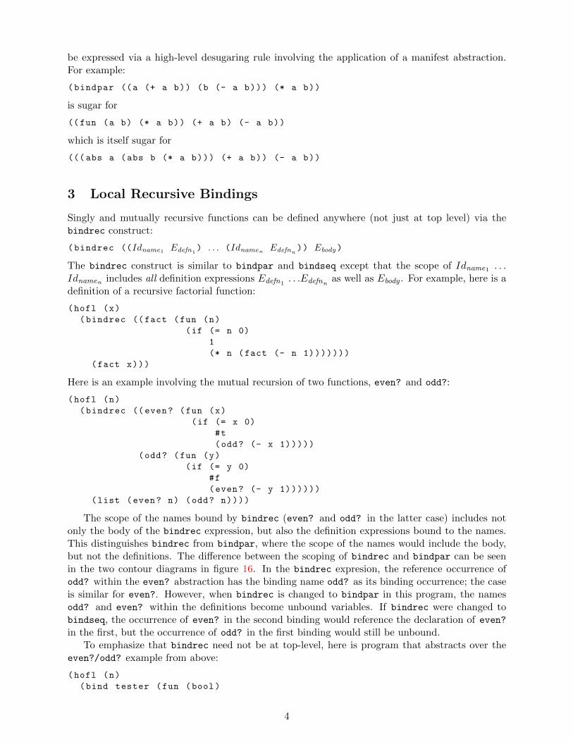
Here is an example involving the mutual recursion of two functions, even? and odd?:

(hofl (n)

(bindrec ((even? (fun (x)

(if (= x 0)

#t

(odd? (- x 1)))))

(odd? (fun (y)

(if (= y 0)

#f

(even? (- y 1))))))

(list (even? n) (odd? n))))

The scope of the names bound by bindrec (even? and odd? in the latter case) includes notonly the body of the bindrec expression, but also the definition expressions bound to the names.This distinguishes bindrec from bindpar, where the scope of the names would include the body,but not the definitions. The difference between the scoping of bindrec and bindpar can be seenin the two contour diagrams in figure 16. In the bindrec expresion, the reference occurrence ofodd? within the even? abstraction has the binding name odd? as its binding occurrence; the caseis similar for even?. However, when bindrec is changed to bindpar in this program, the namesodd? and even? within the definitions become unbound variables. If bindrec were changed tobindseq, the occurrence of even? in the second binding would reference the declaration of even?in the first, but the occurrence of odd? in the first binding would still be unbound.

To emphasize that bindrec need not be at top-level, here is program that abstracts over theeven?/odd? example from above:

(hofl (n)

(bind tester (fun (bool)

4

(hofl (n)

(bindrec ((even? (fun (x)

(if (= x 0)

#t

(odd? (- x 1)))))

(odd? (fun (y)

(if (= y 0)

#f

(even? (- y 1)))))

)

(prep (even? n)

(prep (odd? n)

#e)))

)

C0

C1

C2

C3

(hofl (n)

(bindpar ((even? (fun (x)

(if (= x 0)

#t

(odd? (- x 1)))))

(odd? (fun (y)

(if (= y 0)

#f

(even? (- y 1)))))

)

(prep (even? n)

(prep (odd? n)

#e)))

)

C0

C1

C2

C3

Figure 3: Lexical contours for versions of the even?/odd? program using bindrec and bindpar.

5

(hofl (a b)

(bindrec

(

(map (fun (f xs)

(if (empty? xs)

#e

(prep (f (head xs))

(map f (tail xs))))))

(filter (fun (pred xs)

(cond ((empty? xs) #e)

((pred (head xs))

(prep (head xs) (filter pred (tail xs))))

(else (filter pred (tail xs))))))

(foldr (fun (binop null xs)

(if (empty? xs)

null

(binop (head xs) (foldr binop null (tail xs))))))

(gen (fun (next done? seed)

(if (done? seed)

#e

(prep seed (gen next done? (next seed))))))

(range (fun (lo hi) ; includes lo but excludes hi

(gen (fun (x) (+ x 1)) (fun (y) (>= y hi)) lo)))

(sq (fun (i) (* i i)))

(even? (fun (n) (= (% n 2) 0)))

)

(foldr (fun (x y) (+ x y))

0

(map sq (filter even? (range a (+ b 1)))))))

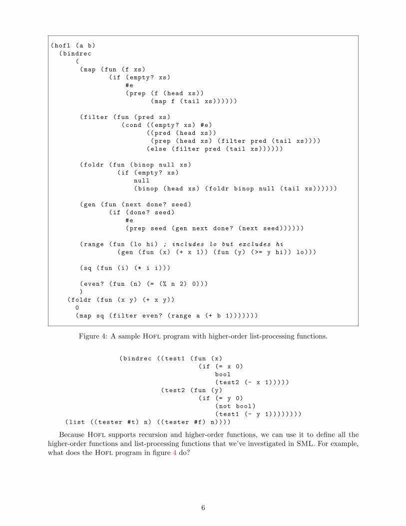
Figure 4: A sample Hofl program with higher-order list-processing functions.

(bindrec (( test1 (fun (x)

(if (= x 0)

bool

(test2 (- x 1)))))

(test2 (fun (y)

(if (= y 0)

(not bool)

(test1 (- y 1))))))))

(list (( tester #t) n) (( tester #f) n))))

Because Hofl supports recursion and higher-order functions, we can use it to define all thehigher-order functions and list-processing functions that we’ve investigated in SML. For example,what does the Hofl program in figure 4 do?

6

4 Definitions in Hofl Programs

To simplify the definition of values, especially functions, in Hofl programs and in the interactiveHofl interpreter, Hofl supports syntactic sugar for top-level program definitions. For example,the fact and even?/odd? examples can also be expressed as follows:

(hofl (x) (fact x)

(def (fact n)

(if (= n 0)

1

(* n (fact (- n 1))))))

(hofl (n) (list (even? n) (odd? n))

(def (even? x)

(if (= x 0)

#t

(odd? (- x 1))))

(def (odd? y)

(if (= y 0)

#f

(even? (- y 1)))))

The Hofl read-eval-print loop (REPL) accepts definitions as well as expressions. All definitionsare considered to be mutually recursive. Any expression submitted to the REPL is evaluated in thecontext of a bindrec derived from all the definitions submitted so far. If there has been more thanone definition with a given name, the most recent definition with that name is used. For example,consider the following sequence of REPL interactions:

hofl > (def three (+ 1 2))

three

For a definition, the response of the interpreter is the defined name. This can be viewed as anacknowledgement that the definition has been submitted. The body expression of the definition isnot evaluated yet, so if it contains an error or infinite loop, there will be no indication of this untilan expression is submitted to the REPL later.

hofl > (+ three 4)

7

When the above expression is submitted, the result is the value of the following expression:

(bindrec ((three (+ 1 2)))

(+ three 4))

Now let’s define a function and then invoke it:

hofl > (def (sq x) (* x x))

sq

hofl > (sq three)

9

The value 9 is the result of evaluating the following expression, which results from collecting theoriginal expression and two definitions into a bindrec and desugaring:

(bindrec ((three (+ 1 2))

(sq (abs x (* x x))))

(sq three))

Let’s define one more function and invoke it:

7

hofl > (def (sum-squares-between lo hi)

(if (> lo hi)

0

(+ (sq lo) (sum-squares-between (+ lo 1) hi))))

sum-squares-between

hofl > (sum-squares-between three 5)

50

The value 50 is the result of evaluating the following expression, which results from collecting theoriginal expression and three definitions into a bindrec and desugaring:

(bindrec ((three (+ 1 2))

(sq (abs x (* x x)))

(sum-squares-between

(abs lo

(abs hi

(if (> lo hi)

0

(+ (sq lo) (( sum-squares-between (+ lo 1)) hi)))))))

(( sum-squares-between three) 5))

It isn’t necessary to define sq before sum-square-between. The definitions can appear in anyorder, as long as no attempt is made to find the value of a defined name before it is defined.

5 Loading Definitions From Files

Typing sequences of definitions into the Hofl REPL can be tedious for any program that containsmore than a few definitions. To facilitate the construction and testing of complex programs, Hoflsupports the loading of definitions from files. Suppose that filename is a string literal (i.e., acharacter sequence delimited by double quotes) naming a file that contains a sequence of Hofldefinitions. In the REPL, entering the directive (load filename) has the same effect as manuallyentering all the definitions in the file named filename. For example, suppose that the file named"option.hfl" contains the definitions in figure 5 and "list-utils.hfl" contains the definitionsin figure 6. Then we can have the following REPL interactions:

hofl > (load "option.hfl")

none

none?

some?

When a load directive is entered, the names of all definitions in the loaded file are displayed. Thesedefinitions are not evaluated yet, only collected for later.

hofl > (none? none)

#t

hofl > (some? none)

#f

hofl > (load "list-utils.hfl")

length

rev

first

second

third

fourth

map

8

(def none (sym *none*)) ; Use symbol *none* to represent the none value.

(def (none? v)

(if (sym? v)

(sym= v none)

#f))

(def (some? v) (not (none? v)))

Figure 5: The contents of the file "option.hfl" which contains an SML-like option data structureexpressed in Hofl.

filter

gen

range

foldr

foldr2

hofl > (range 3 8)

(list 3 4 5 6 7)

hofl > (map (fun (x) (* x x)) (range 3 8))

(list 9 16 25 36 49)

hofl > (foldr (fun (a b) (+ a b)) 0 (range 3 8))

25

hofl > (filter some? (map (fun (x) (if (= 0 (% x 2)) x none)) (range 3 8)))

(list 4 6)

In Hofl, a load directive may appear whereever a definition may appear. It denotes thesequence of definitions contains in the named file. For example, loaded files may themselves containload directives for loading other files. The environment implementation in figure 7 loads thefiles "option.hfl" and "list-utils.hfl". load directives may also appear directly in a Hoflprogram. For example:

(hofl (a b)

(filter some? (map (fun (x) (if (= 0 (% x 2)) x none))

(range a (+ b 1))))

(load "option.hfl")

(load "list-utils.hfl"))

When applied to the argument list [3, 7], this program yields a Hofl list containing the integers4 and 6.

Hofl is even powerful enough for writing interpreters. For example, we can write an Intex,Bindex, and Valex interpreters in Hofl. We can even (gasp!) we write a Hofl interpreter inHofl. Such an interpreter is known as a metacircular interpreter.

6 A Bindex Interpreter Written in Hofl

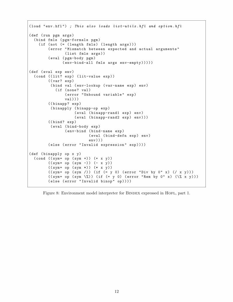
To illustrate that Hofl is suitable for defining complex programs, in figures 8 and 9 we present acomplete interpreter for the Bindex language written in Hofl. Bindex expressions and programsare represented as tree structures encoded via Hofl lists, symbols, and integers. For example, theBindex averaging program can be expressed as the following Hofl list:

9

(def (length xs)

(if (empty? xs)

0

(+ 1 (length (tail xs)))))

(def (rev xs)

(bindrec ((loop (fun (old new)

(if (empty? old)

new

(loop (tail old) (prep (head old) new))))))

(loop xs #e)))

(def first (fun (xs) (nth 1 xs)))

(def second (fun (xs) (nth 2 xs)))

(def third (fun (xs) (nth 3 xs)))

(def fourth (fun (xs) (nth 4 xs)))

(def (map f xs)

(if (empty? xs)

#e

(prep (f (head xs))

(map f (tail xs)))))

(def (filter pred xs)

(cond ((empty? xs) #e)

((pred (head xs))

(prep (head xs) (filter pred (tail xs))))

(else (filter pred (tail xs)))))

(def (gen next done? seed)

(if (done? seed)

#e

(prep seed (gen next done? (next seed)))))

(def (range lo hi) ; includes lo but excludes hi

(gen (fun (x) (+ x 1)) (fun (y) (>= y hi)) lo))

(def (foldr binop null xs)

(if (empty? xs)

null

(binop (head xs)

(foldr binop null (tail xs)))))

(def (foldr2 ternop null xs ys)

(if (|| (empty? xs) (empty? ys))

null

(ternop (head xs)

(head ys)

(foldr2 ternop null (tail xs) (tail ys)))))

Figure 6: The contents of the file "list-utils.hfl" which contains some classic list functionsexpressed in Hofl.

10

(load "option.hfl")

(load "list-utils.hfl")

(def env-empty (fun (name) none))

(def (env-bind name val env)

(fun (n)

(if (sym= n name) val (env n))))

(def (env-bind-all names vals env)

(foldr2 env-bind env names vals))

(def (env-lookup name env) (env name))

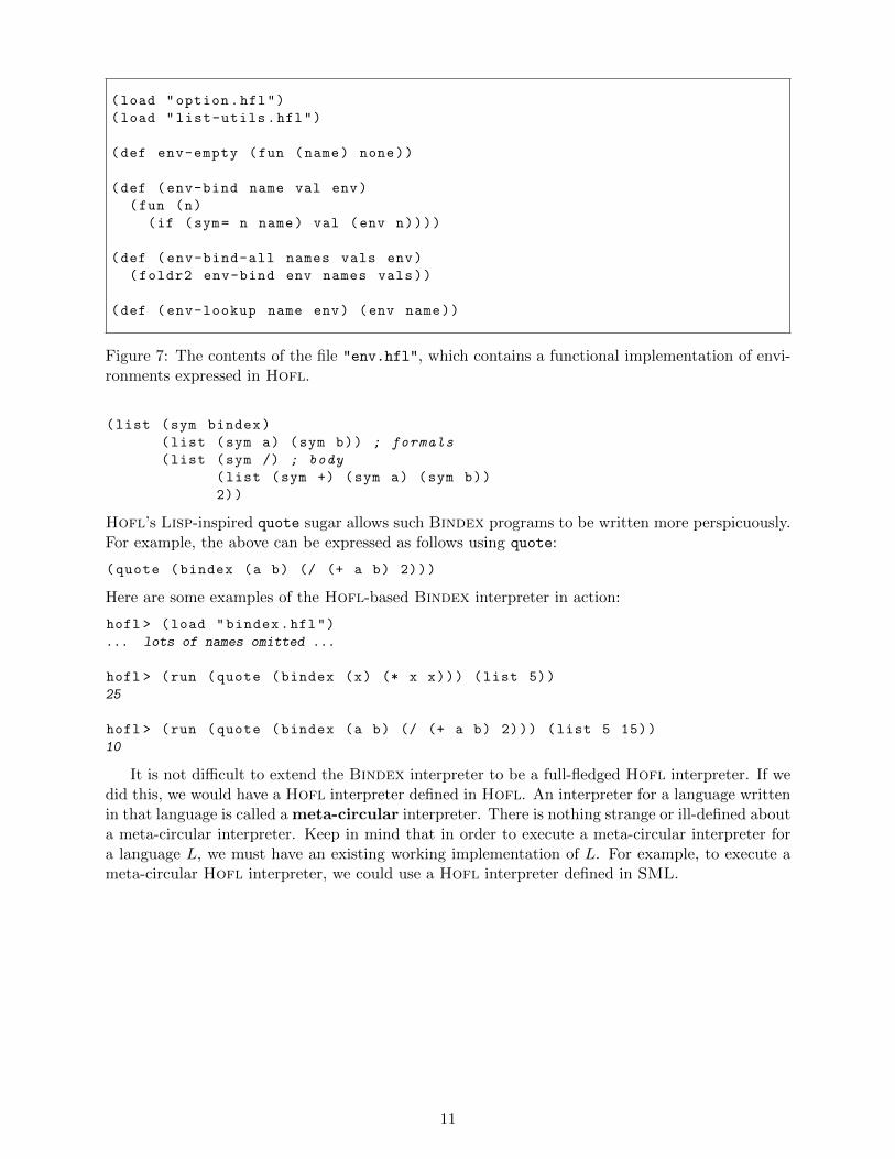
Figure 7: The contents of the file "env.hfl", which contains a functional implementation of envi-ronments expressed in Hofl.

(list (sym bindex)

(list (sym a) (sym b)) ; formals

(list (sym /) ; body

(list (sym +) (sym a) (sym b))

2))

Hofl’s Lisp-inspired quote sugar allows such Bindex programs to be written more perspicuously.For example, the above can be expressed as follows using quote:

(quote (bindex (a b) (/ (+ a b) 2)))

Here are some examples of the Hofl-based Bindex interpreter in action:

hofl > (load "bindex.hfl")

... lots of names omitted ...

hofl > (run (quote (bindex (x) (* x x))) (list 5))

25

hofl > (run (quote (bindex (a b) (/ (+ a b) 2))) (list 5 15))

10

It is not difficult to extend the Bindex interpreter to be a full-fledged Hofl interpreter. If wedid this, we would have a Hofl interpreter defined in Hofl. An interpreter for a language writtenin that language is called a meta-circular interpreter. There is nothing strange or ill-defined abouta meta-circular interpreter. Keep in mind that in order to execute a meta-circular interpreter fora language L, we must have an existing working implementation of L. For example, to execute ameta-circular Hofl interpreter, we could use a Hofl interpreter defined in SML.

11

(load "env.hfl") ; This also loads list-utils.hfl and option.hfl

(def (run pgm args)

(bind fmls (pgm-formals pgm)

(if (not (= (length fmls) (length args)))

(error "Mismatch between expected and actual arguments"

(list fmls args))

(eval (pgm-body pgm)

(env-bind-all fmls args env-empty)))))

(def (eval exp env)

(cond ((lit? exp) (lit-value exp))

((var? exp)

(bind val (env-lookup (var-name exp) env)

(if (none? val)

(error "Unbound variable" exp)

val)))

(( binapp? exp)

(binapply (binapp-op exp)

(eval (binapp-rand1 exp) env)

(eval (binapp-rand2 exp) env)))

((bind? exp)

(eval (bind-body exp)

(env-bind (bind-name exp)

(eval (bind-defn exp) env)

env)))

(else (error "Invalid expression" exp))))

(def (binapply op x y)

(cond ((sym= op (sym +)) (+ x y))

((sym= op (sym -)) (- x y))

((sym= op (sym *)) (* x y))

((sym= op (sym /)) (if (= y 0) (error "Div by 0" x) (/ x y)))

((sym= op (sym \%)) (if (= y 0) (error "Rem by 0" x) (\% x y)))

(else (error "Invalid binop" op))))

Figure 8: Environment model interpreter for Bindex expressed in Hofl, part 1.

12

;;;----------------------------------------------------------------------

;;; Abstract syntax

;;; Programs

(def (pgm? exp)

(&& (list? exp)

(&& (= (length exp) 3)

(sym= (first exp) (sym bindex)))))

(def (pgm-formals exp) (second exp))

(def (pgm-body exp) (third exp))

;;; Expressions

;; Literals

(def (lit? exp) (int? exp))

(def (lit-value exp) exp)

;; Variables

(def (var? exp) (sym? exp))

(def (var-name exp) exp)

;; Binary Applications

(def (binapp? exp)

(&& (list? exp)

(&& (= (length exp) 3)

(binop? (first exp)))))

(def (binapp-op exp) (first exp))

(def (binapp-rand1 exp) (second exp))

(def (binapp-rand2 exp) (third exp))

;; Local Bindings

(def (bind? exp)

(&& (list? exp)

(&& (= (length exp) 4)

(&& (sym= (first exp) (sym bind))

(sym? (second exp))))))

(def (bind-name exp) (second exp))

(def (bind-defn exp) (third exp))

(def (bind-body exp) (fourth exp))

;; Binary Operators

(def (binop? exp)

(|| (sym= exp (sym +))

(|| (sym= exp (sym -))

(|| (sym= exp (sym *))

(|| (sym= exp (sym /))

(sym= exp (sym \%)))))))

Figure 9: Environment model interpreter for Bindex expressed in Hofl, part 2.

13

7 Scoping Mechanisms

In order to understand a program, it is essential to understand the meaning of every name. Thisrequires being able to reliably answer the following question: given a reference occurrence of aname, which binding occurrence does it refer to?

In many cases, the connection between reference occurrences and binding occurrences is clearfrom the meaning of the binding constructs. For instance, in the Hofl abstraction

(fun (a b) (bind c (+ a b) (div c 2)))

it is clear that the a and b within (+ a b) refer to the parameters of the abstraction and that thec in (div c 2) refers to the variable introduced by the bind expression.

However, the situation becomes murkier in the presence of functions whose bodies have freevariables. Consider the following Hofl program:

(hofl (a)

(bind add-a (fun (x) (+ x a))

(bind a (+ a 10)

(add-a (* 2 a)))))

The add-a function is defined by the abstraction (fun (x) (+ x a)), which has a free variablea. The question is: which binding occurrence of a in the program does this free variable refer to?Does it refer to the program parameter a or the a introduced by the bind expression?

A scoping mechanism determines the binding occurrence in a program associated with a freevariable reference within a function body. In languages with block structure1 and/or higher-orderfunctions, it is common to encounter functions with free variables. Understanding the scopingmechanisms of such languages is a prerequisite to understand the meanings of programs written inthese languages.

We will study two scoping mechanisms in the context of the Hofl language: static scoping(section 8) and dynamic scoping (section 9) . To simplify the discussion, we will initially considerHofl programs that do not use the bindrec construct. Then we will study recursive bindings inmore detail in section ??).

8 Static Scoping

8.1 Contour Model

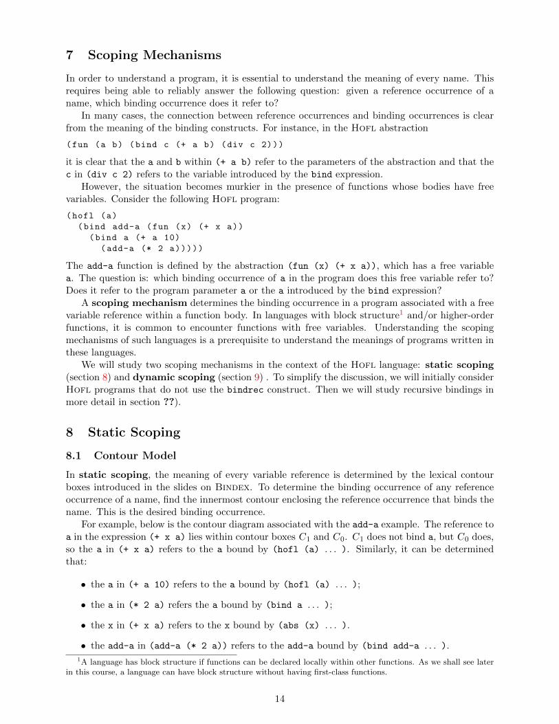
In static scoping, the meaning of every variable reference is determined by the lexical contourboxes introduced in the slides on Bindex. To determine the binding occurrence of any referenceoccurrence of a name, find the innermost contour enclosing the reference occurrence that binds thename. This is the desired binding occurrence.

For example, below is the contour diagram associated with the add-a example. The reference toa in the expression (+ x a) lies within contour boxes C1 and C0. C1 does not bind a, but C0 does,so the a in (+ x a) refers to the a bound by (hofl (a) . . . ). Similarly, it can be determinedthat:

• the a in (+ a 10) refers to the a bound by (hofl (a) . . . );

• the a in (* 2 a) refers the a bound by (bind a . . . );

• the x in (+ x a) refers to the x bound by (abs (x) . . . ).

• the add-a in (add-a (* 2 a)) refers to the add-a bound by (bind add-a . . . ).1A language has block structure if functions can be declared locally within other functions. As we shall see later

in this course, a language can have block structure without having first-class functions.

14

(hofl (a)

(bind add-a (fun (x) (+ x a))

(bind a (+ a 10)

(add-a (* 2 a))) ) )

C1

C3

C0

C2

Static scoping is also known as lexical scoping because the meaning of any reference occurrenceis apparent from the lexical structure of the program.

As another example of a contour diagram, consider the contours associated with the followingprogram containing a create-sub function:

(hofl (n)

(bind create-sub (fun (n) (fun (x) (- x n)) )

(bindpar ((sub2 (create-sub 2))

(sub3 (create-sub 3)))

(bind test (fun (n) (sub2 (sub3 (- n 1))))

(test (sub3 (+ n 1)))

)

)

)

)

C1

C2

C0

C3

C4

C6

C5

By the rules of static scope:

• the n in (- x n) refers to the n bound by the (fun (n) . . . ) of create-sub;

• the n in (- n 1) refers to the n bound by the (fun (n) . . . ) of test;

• the n in (+ n 1) refers to the n bound by (hofl (n) . . . ).

8.2 Substitution Model

The same substitution model used to explain the evaluation of Ocaml, Bindex, and Valex can beused to explain the evaluation of statically scoped Hofl expressions that do not contain bindrec.(Handling bindrec is tricky in the substitution model, and will be considered later.)

For example, suppose we run the program containing the add-a function on the input 3. Thenthe substitution process yields:

(hofl (a)

(bind add-a (fun (x) (+ x a))

(bind a (+ a 10)

(add-a (* 2 a))))) run on [3]; Here and below, assume a ‘‘smart’’ substitution that

; performs renaming only when variable capture is possible.

⇒ (bind add-a (fun (x) (+ x 3))

(bind a (+ 3 10)

15

(add-a (* 2 a))))

⇒∗ (bind a 13 ((fun (x) (+ x 3)) (* 2 a)))

⇒ ((fun (x) (+ x 3)) (* 2 13))

⇒ ((fun (x) (+ x 3)) 26)

⇒ (+ 26 3)

⇒ 29

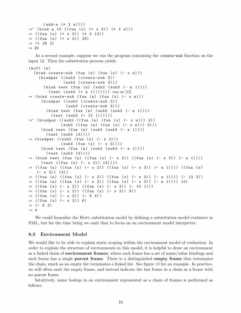
As a second example, suppose we run the program containing the create-sub function on theinput 12. Then the substitution process yields:

(hofl (n)

(bind create-sub (fun (n) (fun (x) (- x n)))

(bindpar ((sub2 (create-sub 2))

(sub3 (create-sub 3)))

(bind test (fun (n) (sub2 (sub3 (- n 1))))

(test (sub3 (+ n 1))))))) run on [12]⇒ (bind create-sub (fun (n) (fun (x) (- x n)))

(bindpar ((sub2 (create-sub 2))

(sub3 (create-sub 3)))

(bind test (fun (n) (sub2 (sub3 (- n 1))))

(test (sub3 (+ 12 1))))))

⇒∗ (bindpar ((sub2 ((fun (n) (fun (x) (- x n))) 2))

(sub3 ((fun (n) (fun (x) (- x n))) 3)))

(bind test (fun (n) (sub2 (sub3 (- n 1))))

(test (sub3 13))))

⇒ (bindpar ((sub2 (fun (x) (- x 2)))

(sub3 (fun (x) (- x 3))))

(bind test (fun (n) (sub2 (sub3 (- n 1))))

(test (sub3 13))))

⇒ (bind test (fun (n) ((fun (x) (- x 2)) ((fun (x) (- x 3)) (- n 1))))

(test ((fun (x) (- x 3)) 13))))

⇒ ((fun (n) ((fun (x) (- x 2)) ((fun (x) (- x 3)) (- n 1)))) ((fun (x)

(- x 3)) 13))

⇒ ((fun (n) ((fun (x) (- x 2)) ((fun (x) (- x 3)) (- n 1)))) (- 13 3))

⇒ ((fun (n) ((fun (x) (- x 2)) ((fun (x) (- x 3)) (- n 1)))) 10)

⇒ ((fun (x) (- x 2)) ((fun (x) (- x 3)) (- 10 1)))

⇒ ((fun (x) (- x 2)) ((fun (x) (- x 3)) 9))

⇒ ((fun (x) (- x 2)) (- 9 3))

⇒ ((fun (x) (- x 2)) 6)

⇒ (- 6 2)

⇒ 4

We could formalize the Hofl substitution model by defining a substitution model evaluator inSML, but for the time being we omit that to focus on an environment model interpreter.

8.3 Environment Model

We would like to be able to explain static scoping within the environment model of evaluation. Inorder to explain the structure of environments in this model, it is helpful to draw an environmentas a linked chain of environment frames, where each frame has a set of name/value bindings andeach frame has a single parent frame. There is a distinguished empty frame that terminatesthe chain, much as an empty list terminates a linked list. See figure 10 for an example. In practice,we will often omit the empty frame, and instead indicate the last frame in a chain as a frame withno parent frame.

Intuitively, name lookup in an environment represented as a chain of frames is performed asfollows:

16

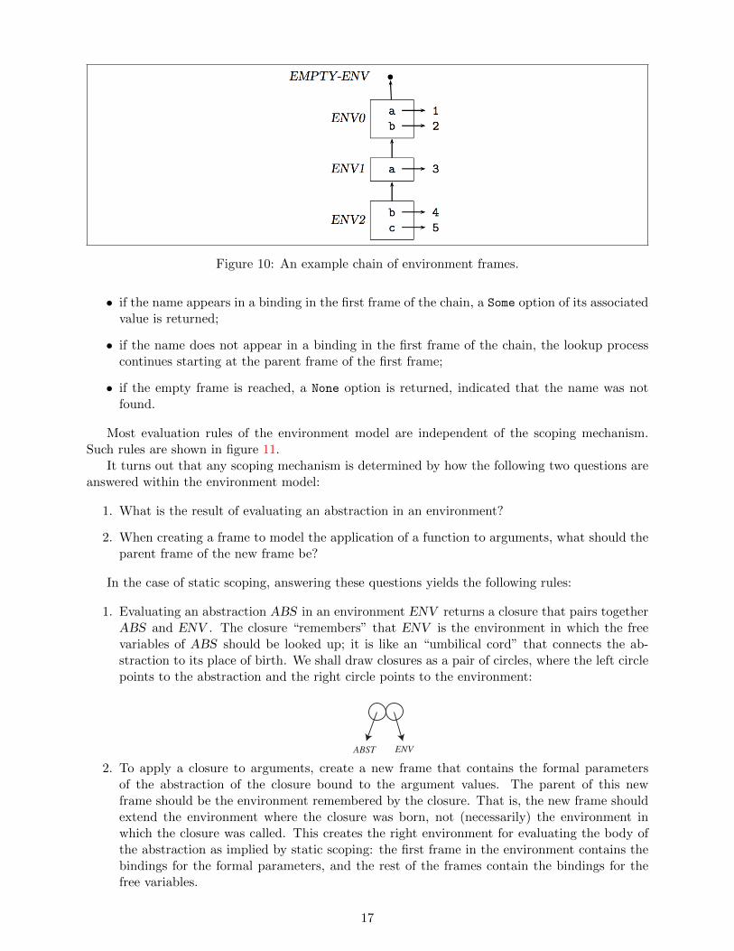
Figure 10: An example chain of environment frames.

• if the name appears in a binding in the first frame of the chain, a Some option of its associatedvalue is returned;

• if the name does not appear in a binding in the first frame of the chain, the lookup processcontinues starting at the parent frame of the first frame;

• if the empty frame is reached, a None option is returned, indicated that the name was notfound.

Most evaluation rules of the environment model are independent of the scoping mechanism.Such rules are shown in figure 11.

It turns out that any scoping mechanism is determined by how the following two questions areanswered within the environment model:

1. What is the result of evaluating an abstraction in an environment?

2. When creating a frame to model the application of a function to arguments, what should theparent frame of the new frame be?

In the case of static scoping, answering these questions yields the following rules:

1. Evaluating an abstraction ABS in an environment ENV returns a closure that pairs togetherABS and ENV . The closure “remembers” that ENV is the environment in which the freevariables of ABS should be looked up; it is like an “umbilical cord” that connects the ab-straction to its place of birth. We shall draw closures as a pair of circles, where the left circlepoints to the abstraction and the right circle points to the environment:

ABST

ENV

2. To apply a closure to arguments, create a new frame that contains the formal parameters

of the abstraction of the closure bound to the argument values. The parent of this newframe should be the environment remembered by the closure. That is, the new frame shouldextend the environment where the closure was born, not (necessarily) the environment inwhich the closure was called. This creates the right environment for evaluating the body ofthe abstraction as implied by static scoping: the first frame in the environment contains thebindings for the formal parameters, and the rest of the frames contain the bindings for thefree variables.

17

Program Running Rule

• To run a Hofl program (hofl (Id1 . . .Idn) Ebody) on integers i1, . . . , ik, return the result ofevaluating Ebody in an environment that binds the formal parameter names Id1 . . .Idn respectivelyto the integer values i1, . . . , ik.

Expression Evaluation Rules

• To evaluate a literal expression in any environment, return the value of the literal.

• To evaluate a variable reference expression Id expression in environment ENV , return the value oflooking up Id in ENV . If Id is not bound in ENV , signal an unbound variable error.

• To evaluate the conditional expression (if E1 E2 E3) in environment ENV , first evaluate E1 inENV to the value V1 . If V1 is true, return the result of evaluating E2 in ENV ; if V1 is false, returnthe result of evaluating E3 in ENV ; otherwise signal an error that V1 is not a boolean.

• To evaluate the primitive application (Orator E1 ... En) in environment ENV , first evaluate theoperand expressions E1 through En in ENV to the values V1 through Vn . Then return the resultof applying the primitive operator Oprimop to the operand values V1 through Vn . Signal an error ifthe number or types of the operand values are not appropriate for Oprimop .

• To evaluate the function application (Efcn Erand) in environment ENV , first evaluate the expres-sions Efcn and Erand in ENV to the values Vfcn and Vrand , respectively. If Vfcn is a function value,return the result of applying Vfcn to the operand value Vrand . (The details of what it means to applya function is at the heart of scoping and, as we shall see, differs among scoping mechanisms.) If Vfcn

is not a a function value, signal an error.

Although bind, bindrec, and bindseq can all be “desugared away”, it is convenient to imagine that thereare rules for evaluating these constructs directly:

• Evaluating (bind Idname Edefn Ebody) in environment ENV is the result of evaluating Ebody inthe environment that results from extending ENV with a frame containing a single binding betweenIdname and the value Vdefn that results from evaluating Edefn in ENV .

• A bindpar is evaluated similarly to bind, except that the new frame contains one binding for each ofthe name/defn pairs in the bindpar. As in bind, all defns of bindpar are evaluated in the originalframe, not the extension.

• A bindseq expression should be evaluated as if it were a sequence of nested binds.

Figure 11: Environment model evaluation rules that are independent of the scoping mechanism.

We will show these rules in the context of using the environment model to explain executionsof the two programs from above. First, consider running the add-a program on the input 3. Thisevaluates the body of the add-a program in an environment ENV 0 binding a to 3:

a

3

ENV0

To evaluate the (bind add-a . . . ) expression, we first evaluate (fun (x) (+ x a)) in ENV 0.According to rule 1 from above, this should yield a closure pairing the abstraction with ENV 0. Anew frame ENV 2 should then be created binding add-a to the closure:

18

a

3

ENV0

add-a

(fun (x) (+ x a))

ENV2

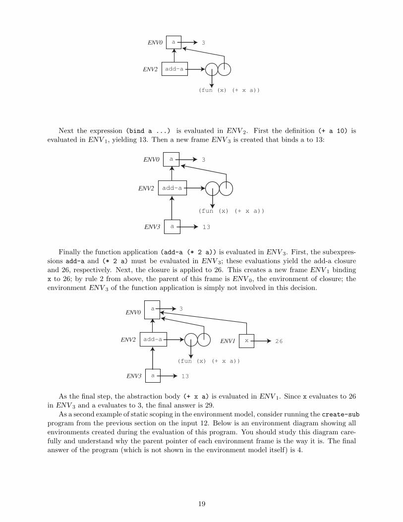
Next the expression (bind a ...) is evaluated in ENV 2. First the definition (+ a 10) isevaluated in ENV 1, yielding 13. Then a new frame ENV 3 is created that binds a to 13:

a

3

ENV0

add-a

(fun (x) (+ x a))

ENV2

a

13

ENV3

Finally the function application (add-a (* 2 a)) is evaluated in ENV 3. First, the subexpres-sions add-a and (* 2 a) must be evaluated in ENV 3; these evaluations yield the add-a closureand 26, respectively. Next, the closure is applied to 26. This creates a new frame ENV 1 bindingx to 26; by rule 2 from above, the parent of this frame is ENV 0, the environment of closure; theenvironment ENV 3 of the function application is simply not involved in this decision.

a

3

ENV0

add-a

(fun (x) (+ x a))

ENV2

a

13

ENV3

x

26

ENV1

As the final step, the abstraction body (+ x a) is evaluated in ENV 1. Since x evaluates to 26in ENV 3 and a evaluates to 3, the final answer is 29.

As a second example of static scoping in the environment model, consider running the create-subprogram from the previous section on the input 12. Below is an environment diagram showing allenvironments created during the evaluation of this program. You should study this diagram care-fully and understand why the parent pointer of each environment frame is the way it is. The finalanswer of the program (which is not shown in the environment model itself) is 4.

19

n

12

ENV0

ENV3

ENV4

n

create-sub

sub2

sub3

2

n

3

(fun (n)

(fun (x)

(- x n)))

(fun (x) (- x n))

ENV1b

ENV1a

ENV6

test

(abs (n) (sub2 (sub3 (- n 1))))

x

13

ENV2a

n

10

x

9

ENV2b

x

ENV2c

6

ENV5

In both of the above environment diagrams, the environment names have been chosen to un-derscore a critical fact that relates the environment diagrams to the contour diagrams. Wheneverenvironment frame ENV i has a parent pointer to environment frame ENV j in the environmentmodel, the corresponding contour C i is nested directly inside of C j within the contour model. Forexample, the environment chain ENV 6 → ENV 4 → ENV 3 → ENV 0 models the contour nestingC6 → C4 → C3 → C0, and the environment chains ENV 2c → ENV 1a → ENV 0, ENV 2a → ENV 1b

→ ENV 0, and ENV 2b → ENV 1b → ENV 0 model the contour nesting C2 →C1 →C0.These correspondences are not coincidental, but by design. Since static scoping is defined by

the contour diagrams, the environment model must somehow encode the nesting of contours. Theenvironment component of closures is the mechanism by which this correspondence is achieved.The environment component of a closure is guaranteed to point to an environment ENVbirth thatmodels the contour enclosing the abstraction of the closure. When the closure is applied, the newlyconstructed frame extends ENVbirth with a new frame that introduces bindings for the parametersof the abstraction. These are exactly the bindings implied by the contour of the abstraction. Anyexpression in the body of the abstraction is then evaluated relative to the extended environment.

8.4 SML Interpreter Implementation of Hofl Environment Model

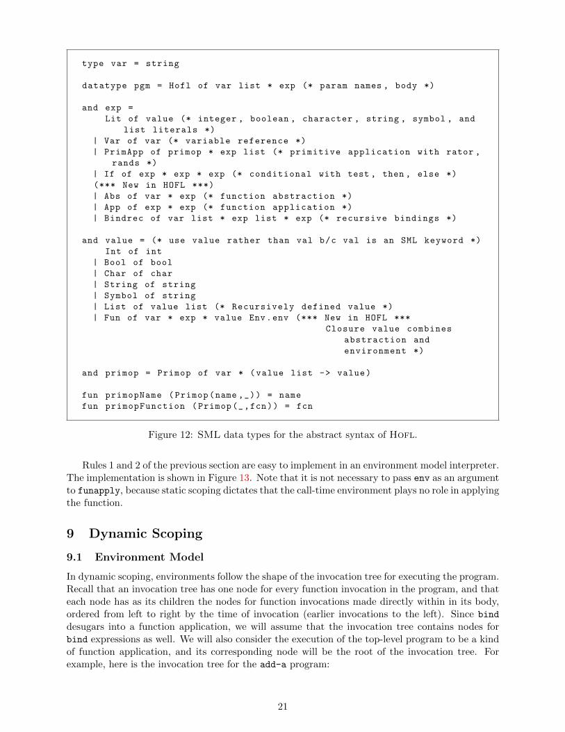
Now we show how to implement the environment model for Hofl in an interpreter written in SML.Figure 12 shows the SML datatypes used in the interpreter. These are similar to Valex except:

• There are new constructors Abs (for unary abstractions), App (for unary applications), andBindrec (for the recursively-scoped bindrec construct).

• There is no need for a Bind constructor, because bind is sugar in Hofl.

• There is a new Fun value for function closures. The third component of a Fun value, anenvironment, plays a very important role in the environment model.

20

type var = string

datatype pgm = Hofl of var list * exp (* param names , body *)

and exp =

Lit of value (* integer , boolean , character , string , symbol , and

list literals *)

| Var of var (* variable reference *)

| PrimApp of primop * exp list (* primitive application with rator ,

rands *)

| If of exp * exp * exp (* conditional with test , then , else *)

(*** New in HOFL ***)

| Abs of var * exp (* function abstraction *)

| App of exp * exp (* function application *)

| Bindrec of var list * exp list * exp (* recursive bindings *)

and value = (* use value rather than val b/c val is an SML keyword *)

Int of int

| Bool of bool

| Char of char

| String of string

| Symbol of string

| List of value list (* Recursively defined value *)

| Fun of var * exp * value Env.env (*** New in HOFL ***

Closure value combines

abstraction and

environment *)

and primop = Primop of var * (value list -> value)

fun primopName (Primop(name ,_)) = name

fun primopFunction (Primop(_,fcn)) = fcn

Figure 12: SML data types for the abstract syntax of Hofl.

Rules 1 and 2 of the previous section are easy to implement in an environment model interpreter.The implementation is shown in Figure 13. Note that it is not necessary to pass env as an argumentto funapply, because static scoping dictates that the call-time environment plays no role in applyingthe function.

9 Dynamic Scoping

9.1 Environment Model

In dynamic scoping, environments follow the shape of the invocation tree for executing the program.Recall that an invocation tree has one node for every function invocation in the program, and thateach node has as its children the nodes for function invocations made directly within in its body,ordered from left to right by the time of invocation (earlier invocations to the left). Since bind

desugars into a function application, we will assume that the invocation tree contains nodes forbind expressions as well. We will also consider the execution of the top-level program to be a kindof function application, and its corresponding node will be the root of the invocation tree. Forexample, here is the invocation tree for the add-a program:

21

(* val eval : Hofl.exp -> value Env.env -> value *)

and eval (Lit v) env = v

...

| eval (Abs(fml ,body)) env = Fun(fml ,body ,env) (* make a closure *)

| eval (App(rator ,rand)) env = apply (eval rator env) (eval rand env)

...

and apply (Fun(fml ,body ,env)) arg = eval body (Env.bind fml arg env)

| apply fcn arg = raise (EvalError ("Non-function rator in

application: " ^ (valueToString fcn)))

Figure 13: Essence of static scoping in Hofl.

run (hofl (a) ...)

bind add-a

invoke add-a

bind a

As a second example, here is the invocation tree for the create-sub program:

run (hofl (n) ...)

bind create-sub

invoke create-sub 2

invoke create-sub 3

bindpar sub2,sub3

bind test

invoke sub3

invoke test

invoke sub3

invoke sub2

Note: in some cases (but not the above two), the shape of the invocation tree may depend onthe values of the arguments at certain nodes, which in turn depends on the scoping mechanism.So the invocation tree cannot in general be drawn without fleshing out the details of the scopingmechanism.

The key rules for dynamic scoping are as follows:

1. Evaluating an abstraction ABS in an environment ENV just returns ABS . In dynamicscoping, there there is no need to pair the abstraction with its environment of creation.

2. To apply a closure to arguments, create a new frame that contains the formal parameters ofthe abstraction of the closure bound to the argument values. The parent of this new frameshould be the environment in which the function application is being evaluated - that is, theenvironment of the invocation (call), not the environment of creation. This means that thefree variables in the abstraction body will be looked up in the environment where the functionis called.

22

Consider the environment model showing the execution of the add-a program on the argument 3in a dynamically scoped version of Hofl. According to the above rules, the following environmentsare created:

a

3

ENV0

add-a

(fun (x) (+ x a))

ENV1

a

13

ENV2

x

26

ENV3

run (hofl (a) ...)

bind add-a

invoke add-a

bind a

The key differences from the statically scoped evaluation are (1) the name add-a is bound toan abstraction, not a closure and (2) the parent frame of ENV 3 is ENV 2, not ENV 0. This meansthat the evaluation of (+ x a) in ENV 3 will yield 39 under dynamic scoping, as compared to 29under static scoping.

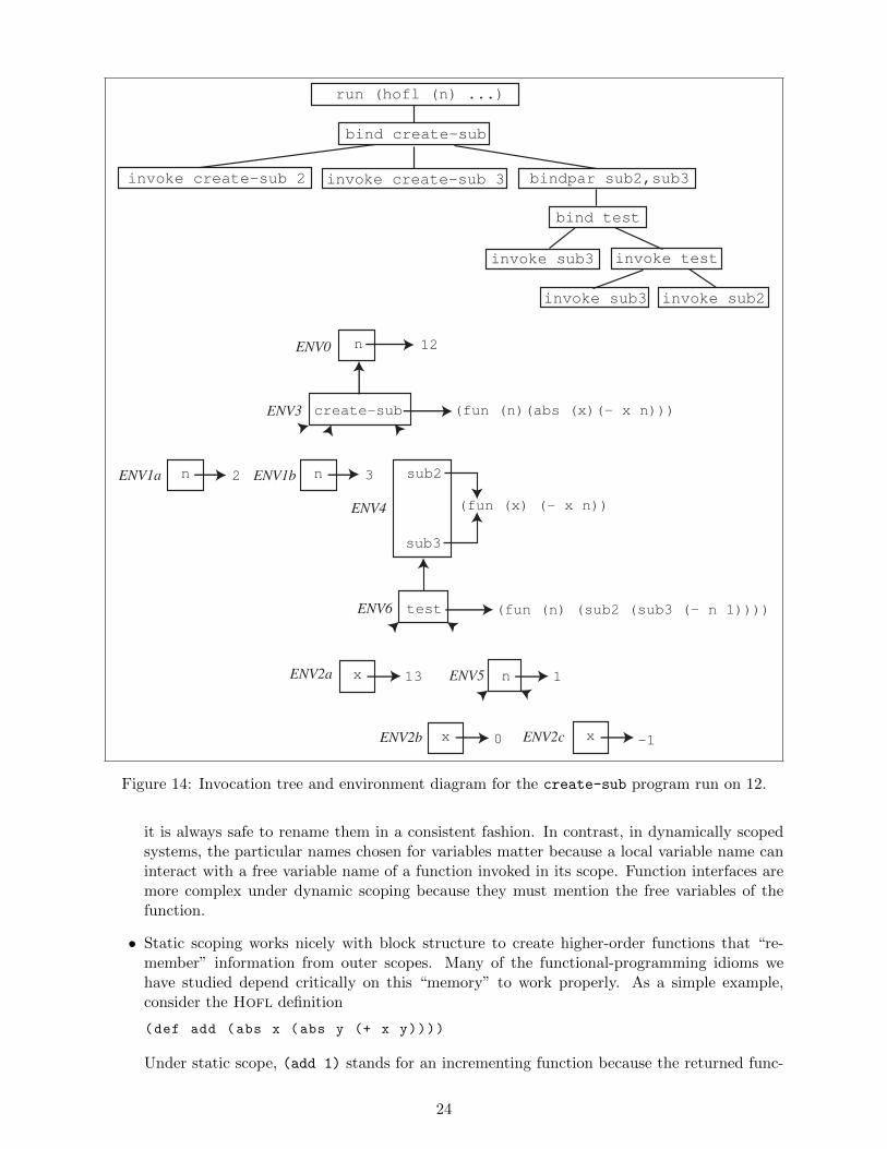
Figure 14 shows an environment diagram showing the environments created when the create-subprogram is run on the input 12. The top of the figure also includes a copy of the invocation tree toemphasize that in dynamic scope the tree of environment frames has exactly the same shape as theinvocation tree. You should study the environment diagram and justify the target of each parentpointer. Under dynamic scoping, the first invocation of sub3 (on 13) yields 1 because the n usedin the subtraction is the program parameter n (which is 12) rather than the 3 used as an argumentto create-sub when creating sub3. The second invocation of sub3 (on 0) yields -1 because the nfound this time is the argument 1 to test. The invocation of sub2 (on -1) finds that n is this same1, and returns -2 as the final result of the program.

9.2 Interpreter Implementation of Dynamic Scope

The two rules of the dynamic scoping mechanism are easy to encode in the environment model.The implementation is shown in Figure 13. For the first rules, the evaluation of an abstractionjust returns the abstraction. For the second rules, the application of a function passes the call-timeenvironment to funapply-dynamic, where it is used as the parent of the environment frame createdfor the application.

9.3 Comparing Static and Dynamic Scope

SNOBOL4, APL, most early Lisp dialects, and many macro languages are dynamically scoped.In each of these languages, a free variable in a function (or macro) body gets its meaning from theenvironment at the point where the function is called rather than the environment at the pointwhere the function is created. Thus, in these languages, it is not possible to determine a uniquedeclaration corresponding to a given free variable reference; the effective declaration depends onwhere the function is called. It is therefore generally impossible to determine the scope of adeclaration simply by considering the abstract syntax tree of the program.

By and large, however, most modern languages use static scoping because, in practice, staticscoping is often preferable to dynamic scoping. There are several reasons for this:

• Static scoping has better modularity properties than dynamic scoping. In a statically scopedlanguage, the particular names chosen for variables in a function do not affect its behavior, so

23

run (hofl (n) ...)

bind create-sub

invoke create-sub 2

invoke create-sub 3

bindpar sub2,sub3

bind test

invoke sub3

invoke test

invoke sub3

invoke sub2

n

12

ENV0

ENV3

ENV4

n

create-sub

sub2

sub3

2

n

3

(fun (n)(abs (x)(- x n)))

(fun (x) (- x n))

ENV1b

ENV1a

test

(fun (n) (sub2 (sub3 (- n 1))))

x

13

ENV2a

n

1

x

-1

ENV2c

x

ENV2b

0

ENV5

ENV6

Figure 14: Invocation tree and environment diagram for the create-sub program run on 12.

it is always safe to rename them in a consistent fashion. In contrast, in dynamically scopedsystems, the particular names chosen for variables matter because a local variable name caninteract with a free variable name of a function invoked in its scope. Function interfaces aremore complex under dynamic scoping because they must mention the free variables of thefunction.

• Static scoping works nicely with block structure to create higher-order functions that “re-member” information from outer scopes. Many of the functional-programming idioms wehave studied depend critically on this “memory” to work properly. As a simple example,consider the Hofl definition

(def add (abs x (abs y (+ x y))))

Under static scope, (add 1) stands for an incrementing function because the returned func-

24

(* val eval : Hofl.exp -> value Env.env -> value *)

and eval (Lit v) env = v

...

| eval (Abs(fml ,body)) env = Fun(fml ,body ,env) (* make a closure *)

| eval (App(rator ,rand)) env = apply (eval rator env) (eval rand env)

env

...

and apply (Fun(fml ,body ,senv)) arg denv = eval body (Env.bind fml arg

denv) (* extend dynamic env *)

| apply fcn arg = raise (EvalError ("Non-function rator in

application: " ^ (valueToString fcn)))

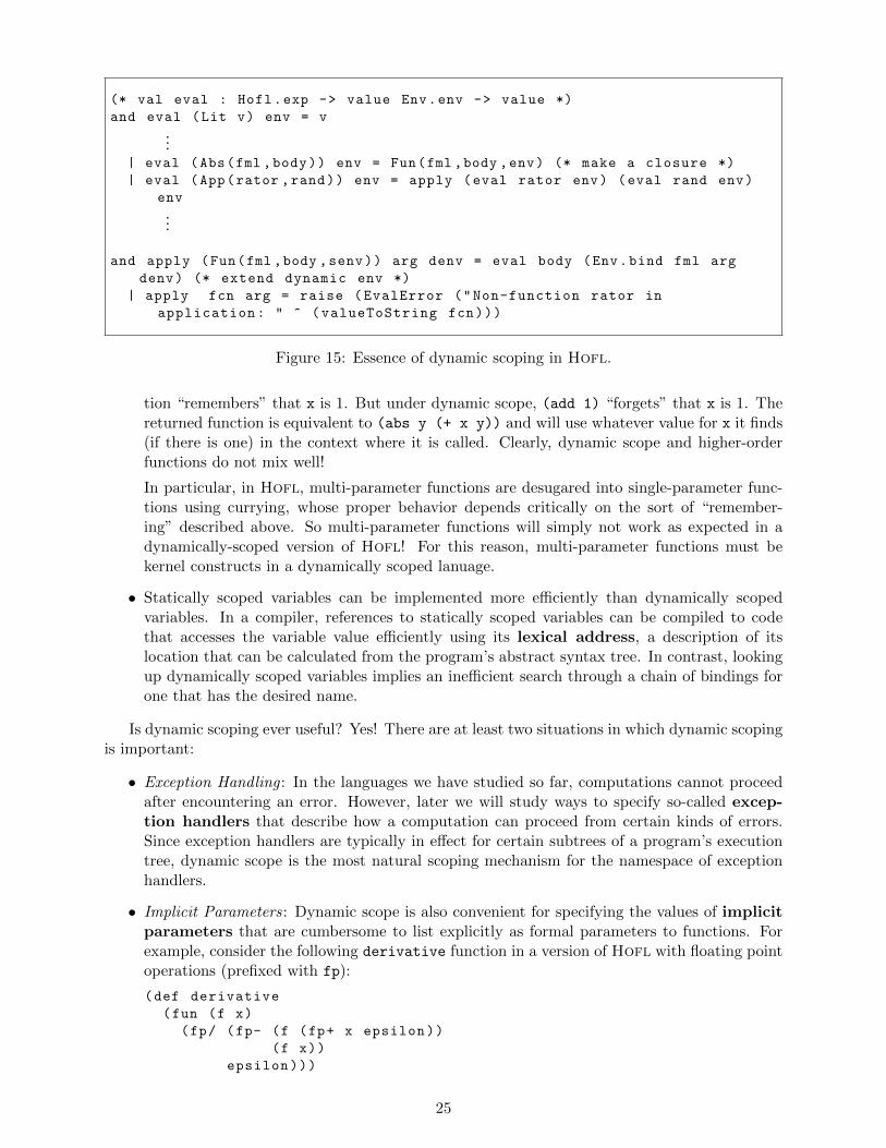
Figure 15: Essence of dynamic scoping in Hofl.

tion “remembers” that x is 1. But under dynamic scope, (add 1) “forgets” that x is 1. Thereturned function is equivalent to (abs y (+ x y)) and will use whatever value for x it finds(if there is one) in the context where it is called. Clearly, dynamic scope and higher-orderfunctions do not mix well!

In particular, in Hofl, multi-parameter functions are desugared into single-parameter func-tions using currying, whose proper behavior depends critically on the sort of “remember-ing” described above. So multi-parameter functions will simply not work as expected in adynamically-scoped version of Hofl! For this reason, multi-parameter functions must bekernel constructs in a dynamically scoped lanuage.

• Statically scoped variables can be implemented more efficiently than dynamically scopedvariables. In a compiler, references to statically scoped variables can be compiled to codethat accesses the variable value efficiently using its lexical address, a description of itslocation that can be calculated from the program’s abstract syntax tree. In contrast, lookingup dynamically scoped variables implies an inefficient search through a chain of bindings forone that has the desired name.

Is dynamic scoping ever useful? Yes! There are at least two situations in which dynamic scopingis important:

• Exception Handling : In the languages we have studied so far, computations cannot proceedafter encountering an error. However, later we will study ways to specify so-called excep-tion handlers that describe how a computation can proceed from certain kinds of errors.Since exception handlers are typically in effect for certain subtrees of a program’s executiontree, dynamic scope is the most natural scoping mechanism for the namespace of exceptionhandlers.

• Implicit Parameters: Dynamic scope is also convenient for specifying the values of implicitparameters that are cumbersome to list explicitly as formal parameters to functions. Forexample, consider the following derivative function in a version of Hofl with floating pointoperations (prefixed with fp):

(def derivative

(fun (f x)

(fp/ (fp- (f (fp+ x epsilon))

(f x))

epsilon)))

25

Note that epsilon appears as a free variable in derivative. With dynamic scoping, it ispossible to dynamically specify the value of epsilon via any binding construct. For example,the expression

(bind epsilon 0.001

(derivative (abs x (fp* x x)) 5.0))

would evaluate (derivative (abs x (fp* x x)) 5.0) in an environment where epsilon

is bound to 0.001.

However, with lexical scoping, the variable epsilon must be defined at top level, and, withoutusing mutation, there is no way to temporarily change the value of epsilon while the programis running. If we really want to abstract over epsilon with lexical scoping, we must pass itto derivative as an explicit argument:

(def derivative

(fun (f x epsilon)

(fp/ (fp- (f (fp+ x epsilon))

(f x))

epsilon)))

But then any procedure that uses derivative and wants to abstract over epsilon mustalso include epsilon as a formal parameter. In the case of derivative, this is only a smallinconvenience. But in a system with a large number of tweakable parameters, the desire forfine-grained specification of variables like epsilon can lead to an explosion in the number offormal parameters throughout a program.

As an example along these lines, consider the huge parameter space of a typical graphicssystem (colors, fonts, stippling patterns, line thicknesses, etc.). It is untenable to specifyeach of these as a formal parameter to every graphics routine. At the very least, all theseparameters can be bundled up into a data structure that represents the graphics state. Butthen we still want a means of executing window routines in a temporary graphics state in sucha way that the old graphics state is restored when the routines are done. Dynamic scoping isone technique for achieving this effect; side effects are another (as we shall see later).

10 Recursive Bindings

10.1 The bindrec Construct

Hofl’s bindrec construct allows creating mutually recursive structures. For example, here is theclassic even?/odd? mutual recursion example expressed in Hofl:

(hofl (n)

(bindrec ((even? (abs x

(if (= x 0)

#t

(odd? (- x 1)))))

(odd? (abs y

(if (= y 0)

#f

(even? (- y 1))))))

(prep (even? n)

(prep (odd? n)

#e))))

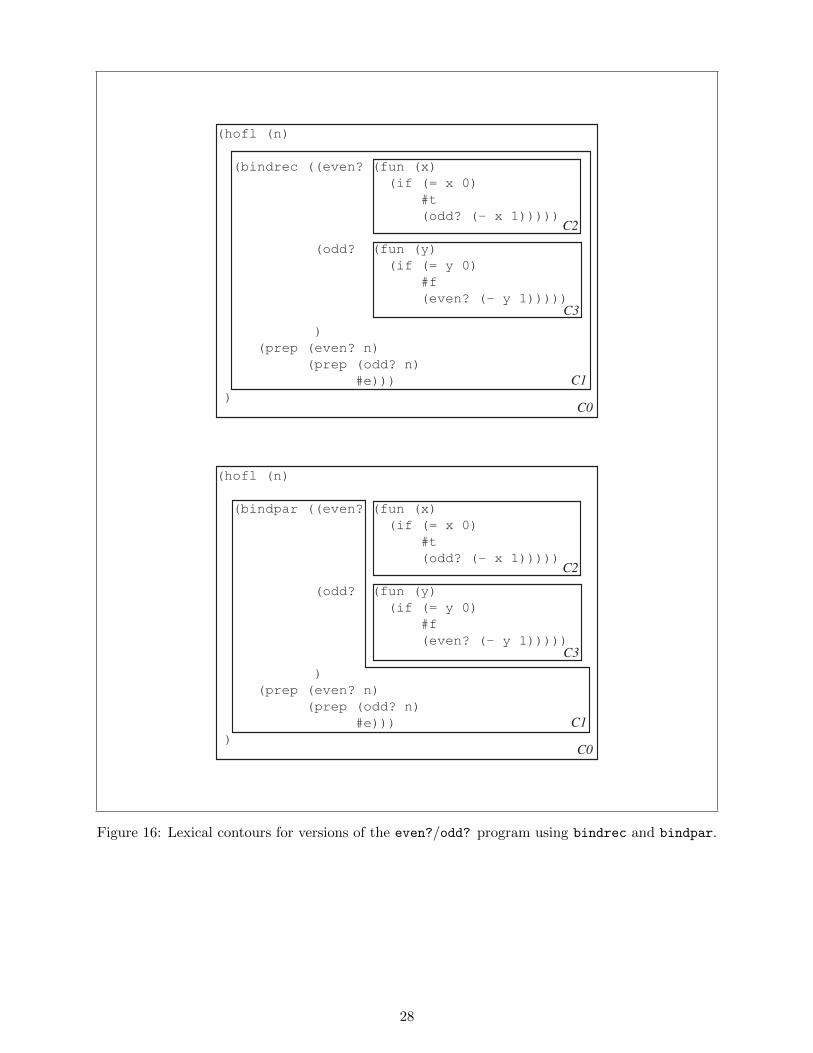
The scope of the names bound by bindrec (even? and odd? in this case) includes not only thebody of the bindrec expression, but also the definition expressions bound to the names. This

26

distinguishes bindrec from bindpar, where the scope of the names would include the body, butnot the definitions. The difference between the scoping of bindrec and bindpar can be seen inthe two contour diagrams in figure 16. In the bindrec expresion, the reference occurrence of odd?within the even? abstraction has the binding name odd? as its binding occurrence; the case issimilar for even?. However, when bindrec is changed to bindpar in this program, the names odd?and even? within the definitions become unbound variables. If bindrec were changed to bindseq,the occurrence of even? in the second binding would reference the declaration of even? in thefirst, but the occurrence of odd? in the first binding would still be unbound.

10.2 Environment-Model Evaluation of bindrec

10.2.1 High-level Model

How is bindrec handled in the environment model? We do it in three stages:

1. Create an empty environment frame that will contain the recursive bindings, and set itsparent pointer to be the environment in which the bindrec expression is evaluated.

2. Evaluate each of the definition expressions with respect to the empty environment. If eval-uating any of the definition expressions requires the value of one of the recursively boundvariables, the evaluation process is said to encounter a black hole and the bindrec is con-sidered ill-defined.

3. Populate the new frame with bindings between the binding names and the values computedin step 2. Adding the bindings effectively “ties the knot” of recursion by making cycles inthe graph structure of the environment diagram.

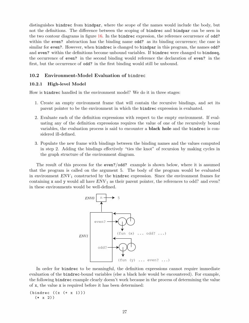
The result of this process for the even?/odd? example is shown below, where it is assumedthat the program is called on the argument 5. The body of the program would be evaluatedin environment ENV 1 constructed by the bindrec expression. Since the environment frames forcontaining x and y would all have ENV 1 as their parent pointer, the references to odd? and even?in these environments would be well-defined.

n

5

even?

odd?

(fun (x) ... odd? ...)

(fun (y) ... even? ...)

ENV0

ENV1

In order for bindrec to be meaningful, the definition expressions cannot require immediateevaluation of the bindrec-bound variables (else a black hole would be encountered). For example,the following bindrec example clearly doesn’t work because in the process of determining the valueof x, the value x is required before it has been determined:

(bindrec ((x (+ x 1)))

(* x 2))

27

(hofl (n)

(bindrec ((even? (fun (x)

(if (= x 0)

#t

(odd? (- x 1)))))

(odd? (fun (y)

(if (= y 0)

#f

(even? (- y 1)))))

)

(prep (even? n)

(prep (odd? n)

#e)))

)

C0

C1

C2

C3

(hofl (n)

(bindpar ((even? (fun (x)

(if (= x 0)

#t

(odd? (- x 1)))))

(odd? (fun (y)

(if (= y 0)

#f

(even? (- y 1)))))

)

(prep (even? n)

(prep (odd? n)

#e)))

)

C0

C1

C2

C3

Figure 16: Lexical contours for versions of the even?/odd? program using bindrec and bindpar.

28

In contrast, in the even?/odd? example we are not asking for the values of even? and odd? inthe process of evaluating the definitions. Rather the definitions are abstractions that will refer toeven? and odd? at a later time, when they are invoked. Abstractions serve as a sort of delayingmechanism that make the recursive bindings sensible.

As a more subtle example of a meaningless bindrec, consider the following:

(bindrec ((a (prep 1 b))

(b (prep 2 a)))

b)

Unlike the above case, here we can imagine that the definition might mean something sensible.Indeed in so-called call-by-need (a.k.a lazy) languages (such as Haskell), definitions like the aboveare very sensible, and stand for the following list structure:

a

b

1

2

However, call-by-value (a.k.a. strict or eager) languages (such as Hofl, Ocaml, Scheme, Java,C, etc.) require that all definitions be completely evaluated to values before they can be bound toa name or inserted in a data structure. In this class of languages, the attempt to evaluate (preps

1 b) fails because the value of b cannot be determined.Nevertheless, by using the delaying power of abstractions, we can get something close to the

above cyclic structure in Hofl. In the following program, the references to the recursive bindingsone-two and two-one are “protected” within abstractions of zero variables (which are known asthunks). Any attempt to use the delayed variables requires applying the thunks to zero arguments(as in the expression ((snd stream)) within the prefix function).

(hofl (n)

(bindpar ((pair (fun (a b) (list a b)))

(fst (fun (pair) (head pair)))

(snd (fun (pair) (head (tail pair)))))

(bindrec (( one-two (pair 1 (fun () two-one)))

(two-one (pair 2 (fun () one-two)))

(prefix (fun (num stream)

(if (= num 0)

(empty)

(prep (fst stream)

(prefix (- num 1)

((snd stream))))))))

(prefix n one-two))))

When the above program is applied to the input 5, the result is (list 1 2 1 2 1).

29