1

Aggregate Electricity demand in South Africa:

Conditional forecasts to 2030

Roula Inglesi1

Department of Economics, Faculty of Economic and Management Sciences, University of Pretoria, Main Campus, Pretoria, 0002, South Africa

Abstract

In 2008, South Africa experienced a severe electricity crisis. Domestic and industrial electricity users had to suffer from black outs all over the country. It is argued that partially the reason was the lack of research on energy, locally. However, Eskom argues that the lack of capacity can only be solved by building new power plants.

The objective of this study is to fill part of the gap of the energy research in the country. By using the Engle Granger methodology for co-integration and Error Correction Models, the variables that explain the aggregate electricity use in South Africa during the period 1980-2005 are examined. Furthermore, we make conditional forecasts of electricity consumption based on the current energy policies

The findings indicate that there is a long run relationship between electricity consumption and price as well as economic growth/income. The last few years in South Africa, price elasticity was rarely taken into account because of the low and decreasing prices in the past. The short-run dynamics of the system are affected by population growth, too

After the energy crisis, Eskom, the national electricity supplier, is in search for substantial funding in order to build new power plants that will help with the envisaged lack of capacity that the company experienced. By using two scenarios for the future of growth, this study shows that the electricity demand will drop substantially due to the price policies agreed –until now- by Eskom and the National Energy Regulator South Africa (NERSA) that will affect the demand for some years.

Keywords: Electricity demand; Forecasting; South Africa

1. Introduction

Since 2007, Eskom, the state owned electricity supplier in South Africa, had experienced a lack of capacity in the generation and reticulation of electricity. As a result, in the first quarter of 2008, blackouts all over the country became common place, with damaging effects on South Africa’s economy. Approximately R50bn were lost from the economy according to National Energy Regulator South Africa (NERSA). [1]

It has been argued that lack of research on electricity and on energy in general [2] in the country has been partially responsible for the predicament of Eskom.

1 Tel: +0124205284 Fax: +30866507249Email address: roula.inglesi@up.ac.za (R. Inglesi)

* Manuscript

2

The situation has been improved during the second quarter. However, Eskom argues that the lack of capacity can only be solved by building new power plants. Is supplying more electricity will solve the problem or the policy makers should follow different strategies in order to avoid similar problems in the future? The objective of this paper is to analyse the aggregate electricity demand by identifying the factors that drive demand. Additionally, by using four conditional scenarios, the future course of electricity consumption is examined.

The rest of the study is organised as follows. In the next section, an analysis of the South African environment is provided. The third section presents a brief literature review of electricity demand studies. The econometric methodology is discussed as well as the data that are used in the following section. Section five explains the empirical results. Finally, a summary of the main points of the study and some policy implications are presented in the Discussion and Conclusion section

2. Background

South Africa is considered to be the most industrialised country of the African continent. Its growth above4% is not on top of the international league but it is better than during the Apartheid years.

During the unstable era of Apartheid, governments accepted different development rates between the black and the white population. These inequalities were depicted in unequal social development as well as growing income inequalities. The disadvantaged majority of the population could not fulfil even their basic needs (food, water, electricity).

In 1978 and 1983, United Nations condemned South Africa at the World Conference Against Racism, and a significant disinvestment movement started, pressuring investors to disinvest from South African companies or companies that did business with South Africa.

In the early 90s, the South Africa’s economy rose again, after the end of the trade sanctions. The trade openness of the country attracted new technology, products and investments. As a result, the economy experienced a boost in all the sectors but, especially in the industrial sector.

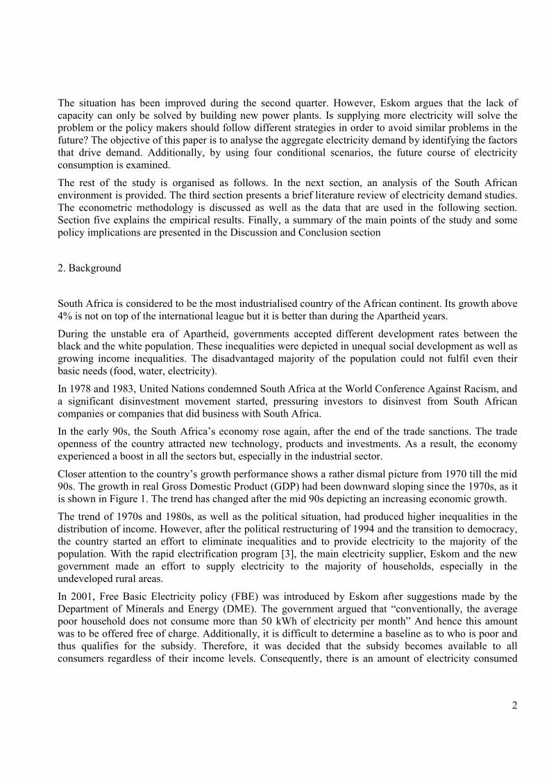
Closer attention to the country’s growth performance shows a rather dismal picture from 1970 till the mid 90s. The growth in real Gross Domestic Product (GDP) had been downward sloping since the 1970s, as it is shown in Figure 1. The trend has changed after the mid 90s depicting an increasing economic growth.

The trend of 1970s and 1980s, as well as the political situation, had produced higher inequalities in the distribution of income. However, after the political restructuring of 1994 and the transition to democracy, the country started an effort to eliminate inequalities and to provide electricity to the majority of the population. With the rapid electrification program [3], the main electricity supplier, Eskom and the new government made an effort to supply electricity to the majority of households, especially in the undeveloped rural areas.

In 2001, Free Basic Electricity policy (FBE) was introduced by Eskom after suggestions made by the Department of Minerals and Energy (DME). The government argued that “conventionally, the average poor household does not consume more than 50 kWh of electricity per month” And hence this amount was to be offered free of charge. Additionally, it is difficult to determine a baseline as to who is poor and thus qualifies for the subsidy. Therefore, it was decided that the subsidy becomes available to all consumers regardless of their income levels. Consequently, there is an amount of electricity consumed

3

that is not connected to price but to the population that use it. The South African population has grown since the 80s with slower rates during the 90s [4]. .

3. Brief literature review

Energy studies have been of great importance the last decade. Most specifically, identifying the factors that drive electricity demand has become crucial for development of the countries, internationally. On the contrary, locally, the electricity research is limited.

In basic economics, the demand for every good/service is usually explained by its own price, income of the buyers, the price of the substitutes and other variables depending on the nature of the good/ service. In the electricity literature, different variables and approaches have been used to model the electricity demand as well as the price and income elasticities. Table I presents a brief summary of some of the important recent studies on the field. Analysing the descriptive statistics of their results for long run price elasticities, we concluded that their mean is -0.48, minimum is -7.4 and maximum is a positive 0.12.

In most studies, income and electricity price are the only variables used to determine electricity demand. In some of them, variations of price are not considered to be explanatory of the demand. [5, 6, 7, 8].

Depending on the nature of the country’s electricity sector, some papers have found the price of substitute significant in their analysis. Possible substitutes were the natural gas, heating oil, bottled gas etc. Those studies assumed that these fuels present perfect substitutability with electricity and that their prices are affordable and preferred rather than electricity from the residential or industrial sector. [9, 10, 11, 12, 13].

To estimate specifically residential demand for electricity, many studies used micro-level data, such as the house size, the household/family size, [9, 10, 11, 14] or number or price of appliances [15]. Westley [14]analysed the residential and commercial demand for electricity in ten regions in Paraguay. By using annual data for the period 1970-1977, he modelled the annual electricity consumption as a function of the real GDP per household, the marginal price of electricity, the house size, the household size and a dummy variable for one of the departments. Both linear and non linear in the parameters models are used.

Due to the nature of residential demand of electricity in some countries, a number of studies [15, 16, 17, 18] have used the weather variations to explain electricity consumption. Zachariadis and Pashourtidou [19] used annual data (1960-2004) to estimate the electricity demand of the residential and service sector of Cyprus. Their model is among those that use the temperature changes as an explanatory variable of the demand due to the weather conditions of the country and found it significant. As a result, “the long term elasticities of electricity use are above the unity and the order of -0.3 and -0.4 for prices. In the short term electricity consumption is rather inelastic, mostly affected by weather fluctuations.”

Murata et al. [20] also support the use of the climate conditions to explain the residential demand. In this study, a questionnaire survey was conducted in 13 cities in China to obtain data specific to the regions and the possession of end-use appliances. The conclusions of the study show that the electricity demand can be reduced by 28% if the appropriate policies for energy efficient households are implemented.

Additionally, some researchers have tried to combine numerous different variables to explain electricity use. [17, 21, 22]. Donatos and Mergos [17] used per capita disposable income, price of electricity, population, price of a substitute of energy, a temperature variable, sales of electrical appliances, the

4

number of consumers and the price of diesel. In the micro level survey data, [23] model electricity consumption as a function of: family size, size of the dwelling, household income, price of electricity and a number of dummies for electrical appliances.

Especially in studies for residential electricity demand, choosing the right price variable is always a complicated question. Instead of an average price per kWh, there is a price schedule from which electricity is purchased in blocks at a marginal price. After having employed different price variables for 25 regions in the Netherlands, Van Helden et al [24] concluded that only average price had the right sign and was statistically significant. Hence, they suggest that the average price should be the only price variable used in the demand function for electricity.

In South Africa in the mid 80s, Pouris [25] attempted to estimate the long run price elasticity of aggregate electricity demand for South Africa by using an unconstrained distributed lag model. He employed annual data for the period 1950-1983 and changes in the electricity price and GDP as explanatory variables. According to the findings of the study, the price elasticity of electricity is -0.90 and the income is considered to be inelastic, as well (0.71).

More recently, Ziramba [8] examines the residential demand for electricity in South Africa for the period 1978-2005. Following the Pesaran et al [26] analysis, he proposed testing for co-integration within an autoregressive distributed framework. The results for the long run income elasticity do not differ substantially from other studies. The income elasticity is positive and estimated to be 0.31. Price elasticity, however, is negative as expected but is statistically insignificant.

For the manipulation of electricity demand and promotion of energy conservation, price electricity can be used as a policy instrument. The estimation of the price elasticity is of high importance for the policy makers. Pouris [25] found a substantial coefficient for the aggregate electricity demand while Ziramba [8]findings indicate that price elasticity is -0.04 but insignificant in the residential sector. Our study will attempt to provide an aggregate estimate that the country needs in order to plan future capacity.

Take Table 1

4. Methodological issues and Data

To model electricity- and generally, energy- demand, co-integration analysis is mostly used in the international literature. Co integration techniques such as those proposed by Engle Granger [31] and Johansen [32] are typically used to identify stationary long run relationships among the variables that would permit the application of standard regression techniques.

The most often used specification of the long run electricity demand is that of a linear double logarithmic form [33]. In the present study, we are following the Engle Granger methodology, according to which the following specification is employed.

Long run:

Electricity demand= α0+α1 income+α2 price of electricity +μ (1)

And the short run:

Electricity demand= β0 + β1 res_coint(-1) + β2 income+ β3 population (all the variables differenced accordingly) (2)

5

Engle and Granger [31] propose a four step procedure if the variables used in the specification are integrated of first order (I(1)):

Step 1: Determine the order of integration of the variables since some co-integration tests are only valid if the variables have the same order of integration. Dickey Fuller (ADF) [34, 35] and Phillips Perron (PP)[35] tests are used to find the degree of integration of the variables used.

Step 2: Estimate the long run equilibrium relationship. For example if we had two variables yt and zt, both integrated of order one, the long-run equilibrium relationship would have the following form:

yt=β0+β1 zt + et (3)

According to the simplest definition of co-integration, two or more variables are co integrated if the residuals of the long run equation are stationary. The auto regression of the residuals has the following form:

Δêt=α1+êt-1+εt (4)

It would be convenient if we could perform a simple Dickey Fuller test on these residuals to determine the order of integration. However, Enders [37] explains why we should not: “...it is not possible to use the Dickey Fuller tables themselves. The problem is that the êt sequence is generated from a regression estimation; the researcher does not know the actual error et, only the estimate of the error êt. The methodology of fitting the regression in (1) selects values β0 and β1 that minimise the sum of squared residuals. Since the residual variance is made as small as possible, the procedure is prejudiced toward finding a stationary error process in (2). Hence the test statistic used to test the magnitude of α1 must reflect this fact.” Therefore, finally, the Standard Dickey Fuller distribution leads to an over rejection of the null hypothesis of no co-integration. Thus, we use critical values calculated according to Mac Kinnon.

Step 3: Estimate the error correction model. If the result of the second step is that there is co-integrationamong the variables then, we use the residuals of the long run equation to estimate the error correction model. Thus, using those residuals, estimate the error correcting model as

Δyt= α1+ αy ê t-1 +Σα 11 (i) Δy t-I + Σ α 12 (i) Δz t-i + ε yt (5)

Step 4: Evaluate the error correction model.

a) The coefficient αy of the lagged residual ê t-1 should be negative. Its size defines the speed of adjustment towards equilibrium relationship.

b) Perform all the appropriate diagnostic tests. Check if the residuals are normally distributed, if there is serial correlation, heteroskedasticity and if the estimation is correctly specified.

Data

Five variables are used in this study: real GDP, real electricity consumption, average electricity price, real disposable income and population. Internationally, reliable sources of data provide data for the electricity consumption only until 2006; with the last figures still subject to change. Therefore, it was preferable to limit the period analysed to 1980-2005 and employ annual data.

The descriptive statistics of the variables as well as the sources of the data are shown in the Appendix, in Tables 2 and 3 respectively.

6

5. Empirical specification

As it was discussed in the literature review, the demand for electricity has been modelled in numerous ways. Concerning the explanatory variables to be included in the analysis, changes in income or Gross Domestic Product (GDP), price of electricity, price of an alternative source of energy (substitute), price of coal (as source of producing electricity) and changes in temperatures are the most commonly used variables.

The individuality of the South African energy system is that the price of coal is strongly linked with the price of electricity. Most of the electricity in South Africa is generated by coal- fired stations (91% in 2000 according to Eskom’s Annual Report) [38]. Therefore, as coal cost is almost 25-30% of the final price of electricity, any high variation in the price of coal will be reflected partially in the price of electricity and multicollinearity problems will exist. In order to confirm this assumption, the correlation coefficient between the price of electricity and price of coal during the period 1980-1996 was estimated. The estimated correlation coefficient is 1, proving our expectations right.

Climate changes are used often in the literature in order to account for seasonal variations in the electricity demand, mostly for the heating of the domestic sector. However, this variable loses its explanatory power in aggregate demand studies because it is very likely that the variation in one sector neutralises by opposite variation. Especially in South Africa, the industrial sector, which is not influenced by the temperature changes, consumes the biggest part of the total electricity consumed in the country.

Additionally, in the country in question, the seasonal temperature variation is minor: among the nine biggest cities, one of each of the nine provinces, the average maximum temperature is 25°C and the average minimum temperature is 12°C.

In energy demand models, usually, the price of a substitute is used to explain the consumption of a commodity. This assumes that the different fuels should be perfect substitutes and can easily replace each other. However, in the case of electricity this is not easily valid because electricity has unique characteristics. Pouris [25] argued in his study: “It (electricity) is the cleanest of all fuels for the end user; it is versatile, easily transferable, and susceptible to fractional use and offers precision of a kind that it is difficult or impossible for fossil fuels processes to match.”

In South Africa, a close –but not perfect- substitute is considered to be the natural gas. Except for the fact that natural gas is not a perfect substitute due to its nature, the prices of the two fuels were also compared. Prices of gas are found to be almost 2.5 times higher than the prices of electricity in average during 1980-2005. The result confirms once more that there is no perfect substitutability because, especially, domestic users are not able to change from electricity to natural gas without increasing their expenses to a large extent.

For the above reasons, it was decided not to use the prices of coal and natural gas and the weather variations in explaining the aggregate electricity demand. In our model, we use a proxy for income, price of electricity and a new introduced variable: the country’s population growth.

In South Africa, before 1994, most of the population did not have access to electricity. The new government recognised that the provision of free basic services is, primarily, a social function that is the responsibility of government. As it was described in Section 2, a national free basic electricity (FBE) policy was introduced to all electricity users in 2001. Since then, there is an amount of electricity used that does not depend on price but on population.

7

Finally, the electricity demand (LCONS) is decided to be estimated as a function of the annual disposable income (LRYD), the real average electricity price (LPRICE_ELEC), the real Gross Domestic Product (LGDP) and the population (LPOP). See Table 4 for units of measurement for the variables used.

Take Table 4

According to economic theory, the coefficient of LRYD and LGDP are expected to be positive since the income elasticity is positive. The coefficient of LPRICE_ELEC is expected to be negative (price elasticity is negative). Finally, the coefficient of LPOP is expected to be positive: the higher the population the higher the electricity demand).

The first step of our analysis is to verify the order of integration of the variables since some co-integrationtests are only valid if the variables have the same order of integration. Dickey Fuller (ADF) and Phillips Perron (PP) tests are used to find the degree of integration of the variables used. Table 5 in the Appendix presents the results of ADF and PP‘s unit roots tests for all economic and electricity variables used in the analysis.

Both ADF and PP tests agree that all the variables are non stationary in values. However, once differenced once, they all become stationary. Our conclusion is that all the variables are of first order of integration, I(1).

The second step is to identify the existence of co-integration using the Engle Granger approach, see Appendix, Table 6. Finally, an Error Correction Model was used to capture the short run dynamics of the model. These techniques render the following result:

Long run:

LCONS=0.415080*LRYD-0.564388*LPRICE_ELEC+7.362757 (6)

(3.678872) (-3.899361) (10.34688)

Short run:

DLCONS=-0.243863*RES_COINT(-1)+0.819622*DLGDP+3.466989*DLPOP-0.049693 (7)

(-2.598878) (3.896051) (4.094198) (0.018494)

The standard variables suggested in the theory to influence technological progress, prove to be significant and with the correct signs. Variables driving electricity demand in the long run are proposed to be the disposable income and the price of electricity. On the other side, the short run dynamics of the system are influenced by the Gross Domestic Product (GDP) and the population.

In order to make sure, that the dynamics shown in the short run model is the correct one, coefficient, residual and stability tests were performed (see Appendix, Table 7) and in order to adjust the long run (co integrating) coefficients for initial bias, the Engle Yoo third step was performed (see Appendix, Table 8).

Interpreting the results of the model economically, in the long run a 10% increase in the price of electricity will decrease the electricity consumption by 5.5%. A 10% increase in the disposable income will increase the electricity demand by 4.2%.

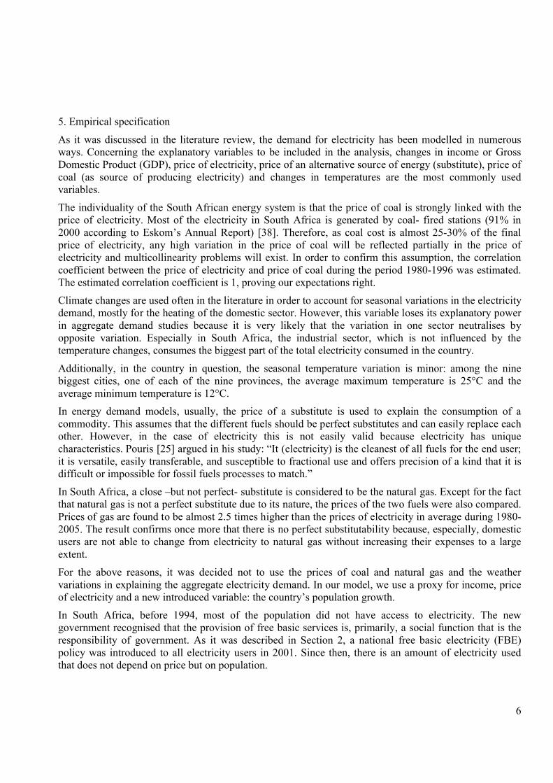
For the purpose of checking the stability and dynamics of the model, a series of dynamic simulations are performed where each of the explanatory variables is subjected to sensitivity testing by increasing (shocking) each of them independently by 10% from 1994 onwards. The effects of these shocks on electricity demand are then calculated. These results are depicted in Figure 2 in the Appendix.

8

Having applied a 10 per cent shock to each of the long run explanatory variables, the dependent variable, electricity consumption, converged to a new equilibrium in the long run. Increases in the electricity prices lead to sustained decreases in the price of electricity. In contrast, increases in the income lead to lasting increases of electricity demand.

6. Forecast to 2030

Following Oztuk and Ceylan [39] approach, two scenarios are introduced to forecast the electricity demand until 2030. Both of them use the predictions of the International Monetary Fund (IMF) about population: 1% increase per annum [4]. At last year’s National Electricity Summit, a real increase of price of about 25% a year was agreed between the National Energy Regulator and Eskom. Therefore, for this exercise, the following assumption holds for both scenarios: the electricity price will increase and double from 2008 to 2011 and then it will remain constant until 2025.

The main difference between the two scenarios is that in the first one, the economic growth will average 4 per cent for the period 2009-2030; whereas, the second one proposes accelerated growth of 6 per cent in average over the period 2009-2030.

The effects of the two forecasts to the electricity consumption until 2030 are presented in Figure 3.

Take Figure 3

Based on IMF calculations and Eskom policies, the electricity consumption for 2030 is estimated to be 148481GWh or 158288GWh according to the first and second scenario respectively. The electricity demand will experience a decrease within the range of 24 to 27 per cent.

It is very important at this point to mention that during the period 2006-2008, the forecasting is ex postand is used for the evaluation of the forecast quality. The latest data that StatsSA [40] released reconfirm the finding of this forecasting activity; the electricity consumption started decreasing in 2008 (monthly data) until February of 2009(latest data). The estimated consumption reduced by 10.2% in February 2009 compared to February 2008.

It is highly noticeable that regardless the level of economic growth chosen, the electricity consumption follows the same trend: decrease for the period while the prices are increasing and start increasing again with low growth rates while the prices are constant.

7. Discussion and Conclusion

After the electricity crisis of 2008, the investigation on the electricity demand had become a necessity. In this paper, the aggregate electricity demand was investigated by employing annual data for the period 1980-2005. With a lack of research on forecasting the electricity demand in South Africa, the objective of our study was to fill the existing gap in the literature and determine the factors that identify the electricity consumption as well as discuss its future.

Applying the Engle Granger co integration technique and Error Correction models, the relationship between the electricity demand and income, prices and population was analysed. Results show that the long term impact of income and price is significant and they are both estimated to be inelastic, 0.42 and -0.55 respectively. Our results are within the range of the results for other countries (see Table 1: median -0.48). In the short run, the demand for electricity is explained by the Gross Domestic Product (GDP) and the size of the population of the country.

9

This investigation has two main differences with Ziramba‘s [8] approach. Firstly, he investigates the residential demand of electricity while our finings are calculated for aggregate demand. A quick look at Table 1 can show that long run price elasticities in aggregate studies are usually smaller than those in residential studies. The long run price elasticity of this study (-0.55) is smaller than Ziramba’s [8] (-0.04) following the international trend. The other difference is the methodological approaches of the two papers. Ziramba [8] used the approach proposed by Pesaran [26] in comparison with this paper where modelling is based on the Engle Granger methodology [31].

As it is shown in Figure 4, the aggregate electricity consumption was increasing until 2005. There are a number of reasons for this trend. Firstly, after the end of sanctions, new technology and investments were attracted and hence, the economic growth had an upward slope from the early 90s. This increase affected the electricity use, especially in the industrial sector.

In the beginning of 90s, only one third of the population had access to electricity. After the transition to democracy, a movement to provide electricity to the rest of the population started. In 2001, the Free Basic Electricity policy was introduced and now, more than two thirds of the population has access to electricity. Therefore, the increase of population added to the raise of electricity demand.

In addition, the real average price of electricity was falling for the last years [41]. This was another factor that increased the energy consumption until 2005.

Two different scenarios were introduced to forecast the electricity demand until 2030. In both of them the population growth was 1% per annum (IMF). For this exercise, the following assumption holds for both scenarios: the electricity price will increase and double from 2008 to 2011 and then it will remain constant until 2025.

The main difference between the two scenarios is that in the first one, the economic growth will average 4 per cent for the period 2009-2030; whereas, the second one proposes accelerated growth of 6 per cent in average over the period 2009-2030.

For the manipulation of electricity demand and promotion of energy conservation, price electricity can be used as a policy instrument. According to the scenarios used, the demand for electricity will decline after the price re structure that is being promoted by Eskom and the National Energy Regulator of South Africa (NERSA). Furthermore, significant forces that drive the fall of the electricity use are also the lower population growth and the lower, more stable, economic growth of the country.

More specifically, South Africa can experience up to 27% decrease of the electricity demand (comparison of 2007 to 2030 values) if the price of electricity double until 2011 and then stay constant with average economic growth equals 4 per cent for the period until 2030. The picture does not differ a lot if the economic growth will be higher up to 6per cent: the electricity demand will drop by 24% by 2030.

In the beginning of the analysis, Eskom was in search for substantial funding in order to build new power plants that will help with the envisaged lack of capacity that the company experienced in the beginning of 2008.

Based on our findings, the needs of Eskom for funding in order to expand current power plant capacity can be questioned. The policy makers can control the electricity demand with the appropriate price policy decisions.

10

8.Appendix

Take Table 2

Order of integration tables with Augmented Dickey-Fuller and Phillips Perron tests

In analysing the univariate characteristics of the data, the Dickey-Fuller (DF) and Augmented Dickey-Fuller tests were employed to establish the order of integration of data series, all variables in natural logarithmic form.

The number of lags used in the estimated equations was determined in a similar way as suggested by Perron (1989:1384), namely starting with eight lags and testing downwards, until the last lag is significant or there are no lags left.

Take Table 5.

Table 5 reports the outcomes of the ADF-tests for all relevant data series employed in the estimations. The series tested are listed in the first column. The second column reports whether a trend and a constant (Trend), only a constant (Constant), or neither one (None) is reported. The next column shows the ADF t-statistic, called ττ when a trend and a constant are included, τμ when only a constant is included, and τ when neither is included. The next column reports the F-statistic, Φ3 (Φ1), testing whether the trend (constant) is significant under the null hypothesis of no unit root and the last column states the conclusion after the test.

Take Table 6

Mac Kinnon critical values:

10%: -3.7412

5%: -4.1502

1%: -5.0207

Since the ADF statistic of -3.91 is smaller than the 10% MacKinnon critical value of -3.74, we can conclude that the res_coint is stationary and therefore the long run equation is indeed cointegrated.

Take Figure 2

Take Table 7

Take Table 8

11

9. References

[1] Mail & Guardian Online. Nersa: Power crisis cost South Africa about R50 million, <http://www.mg.co.za/article/2008-08-26-nersa-power-crisis-cost-sa-about-r50bn>; 2008 [Accessed: 30-3-2009].

[2] A. Pouris, Energy and Fuels Research in South African Universities: A comparative assessment, The Open Inf. Sci. J. 1(2008) ,pp 1-9.

[3] B. Bekker, A. Eberhard, T. Gaunt, A. Marquard, South Africa’s rapid electrification programme: Policy, institutional, planning, financing and technical innovations, Energy Policy 36 (2008), pp 3125-3137.

[4] International Monetary Fund (IMF). World Economic Outlook October. International Monetary Fund Publications; 2008.

[5] Z. Atakhanova, P. Howie, Electricity demand in Kazakhstan, Energy Policy 35 (2007), pp 3729-3743.

[6] G. E. Nasr, E.A. Badr, G. Dibeh, Econometrics modelling of electricity consumption in post war Lebanon, Energy Econ. 22 (2000), pp 627-640.

[7] Narayan P.K, Smyth R, Prasad A. Electricity consumption in G7 countries: A panel co integration analysis of residential demand elasticities, Energy Policy 2007; 35: 4485-4494.

[8] E. Ziramba, The demand for residential electricity in South Africa, Energy Policy 36 (2008), pp 3460-3466.

[9] T. Anderson, C. Hsiao, Formulation and estimation of dynamic models using panel data, J. of Econometrics 18 (1982), pp 578-606.

[10] K. H. Anderson, R. Pomfret, Relative living standards in new market economies: evidence from Central Asian household surveys, J. of Comp. Econ. 30 (2002), pp 683-708.

[11] J.W. Wilson, Residential demand for electricity, Q. Rev. of Econ. and Bus. 11 (1971), pp 7-22.[12] H. S. Houthakker, Some calculations on electricity consumption in Great Britain, J. of the Royal

Stat. Society 114 (1951), pp 359-371.[13] P.K. Narayan, R. Smyth, The residential demand for electricity in Australia: an application of the

bounds testing approach to co-integration, Energy Policy 33 (2005), pp 467-474.[14] G.D. Westley, Electricity Demand in a Developing country, The Rev. of Econ. and Stat. 66 (1984),

pp 459-467.[15] A. Diabi, The demand for electric energy in Saudi Arabia: an empirical investigation, OPEC Rev.

22 (1998), pp 13-29.[16] G. Hondroyiannis, Estimating residential demand for electricity in Greece, Energy Econ. 26

(2004), pp 319-334.[17] G. S. Donatos, G. J. Mergos, Residential demand for electricity: The case of Greece, Energy Econ.

13 (1991), pp 41-47.[18] M.A. Asadoorian, R. Eckaus, C.A. Schlosser, Modelling climate feedbacks to electricity demand:

The case of China, Energy Econ. 30 (2008), pp 1577-1602[19] T. Zachariadis, N. Pashourtidou , An empirical analysis of electricity consumption in Cyprus,

Energy Econ. 29 (2007), pp 183-198.[20] A. Murata, Y. Kondou, M. Hailin, Z. Weisheng, Electricity demand in the Chinese urban

household-sector, Appl. Energy 85 (2008), pp 1113-1125.[21] T. Dergiades, L. Tsoulfidis, Estimating residential demand for electricity in the United States,

1965-2006, Energy Econ. 30 (2008), pp 2722-2730.[22] D. R. Kamerschen, D.V. Porter, The demand for residential, industrial and total electricity, 1973-

1998, Energy Econ. 26 (2004), pp 87-100.

12

[23] S. H. Yoo, J.S. Lee, S.J. Kwak, Estimation of residential electricity demand function in Seoul by correction for sample selection bias, Energy Policy 35 (2007), pp 5702-5707.

[24] G.J. Van Helden, P.S.H. Leeflang, E. Sterken, Estimation of the demand for electricity, Appl.Econ. 19 (1987), pp 69-82.

[25] A. Pouris, The price elasticity of electricity demand in South Africa, Appl. Econ. 19 (1987), pp1269-1277.

[26] M.H. Pesaran, Y. Shin, R.J. Smith, Bounds testing approaches to the analysis of level relationships, J. of Appl. Econometrics 16 (2001), pp 289-326.

[27] J-T. Bernard, D. Bolduc, D. Belanger. Quebec Residential electricity demand: A microeconometric approach, Can. J. of Econ. 29 (1996), pp 92-113.

[28] A.R. Al-Faris, The demand for electricity in the GCC countries, Energy Policy 30 (2002), pp 117-124.

[29] M. Filippini, S. Paschauri, Elasticities of electricity demand in urban Indian households, Appl.Econ. Lett. 6 (1999), pp 533-538.

[30] G. De Vita, K. Endresen, I.C. Hunt, An empirical analysis of energy demand in Namibia, Energy Policy 34 (2006), pp 3447-3463.

[31] R. F. Engle, C.W.J. Granger, Co- integration and Error Correction: Representation, Estimation and Testing, Econometrica 55 (1987), pp 251-267.

[32] S. Johansen, Estimation and Hypothesis Testing of Cointegration Vectors in Gaussian Vector Autoregressive Models, Econometrica 59 (1991), pp 1551-80.

[33] F. Halicioglu, Residential electricity demand dynamics in Turkey, Energy Econ. 29 (2007), pp199-210.

[34] D. A. Dickey, W. A. Fuller, Distributions of the estimators of autoregressive time series with a unit root, J. of the Am. Stat. Assoc. 74 (1979), pp 427-431.

[35] D. A. Dickey, W. A. Fuller, The likelihood ratio statistics for autoregressive time series with a unit root, Econometrica 49 (1981), pp 1057-1072.

[36] P.C.B. Phillips, P. Perron, Testing for a unit root in time series regression, Biometrica 75 (1988), pp 335-346.

[37] Enders W. Applied Econometric Time series. Willey: New York, 2004.[38] Eskom. Annual Report 2000. Pretoria: Eskom publications; 2000.[39] H.K. Oztuk, H. Ceylan, Forecasting Total and Industrial Sector electricity demand based on

genetic algorithm approach: Turkey case study, Int. J. of Energy Res. 29 (2005), pp 829-840.[40] Statistics South Africa. Electricity generated and available for distribution, February 2009.

Pretoria: Statistics South Africa; 2009. [41] Department of Minerals and Energy, Directorate: Energy Planning and Development. Annual

Price Report 2005. Pretoria: Department of Minerals and Energy; 2005.[42] Eskom. Annual Report 2005. Pretoria: Eskom publications; 2005.[43] Department of Minerals and Energy, Electricity Basic services support tariff (Free basic

electricity) Policy. Pretoria: Department of Minerals and Energy; 2003.

Suggested referees

1. Prof A. Pouris. Institute for technological innovation. University of Pretoria2. Prof J. Blignaut. Department of Economics. University of Pretoria3. Kibii Komen, PhD candidate, University of Pretoria

* Suggested Referees

Figure 1Click here to download high resolution image

Figure 2a 2bClick here to download high resolution image

Figure 2c 2dClick here to download high resolution image

Figure 3Click here to download high resolution image

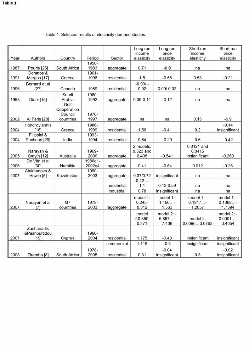
Table 1: Selected results of electricity demand studies.

Year Authors Country Period Sector

Long run income

elasticity

Long run price

elasticity

Short run income

elasticity

Short run price

elasticity

1987 Pouris [25] South Africa1950-1983 aggregate 0.71 -0.9 na na

1991Donatos &

Mergos [17] Greece1961-1996 residential 1.5 -0.58 0.53 -0.21

1996Bernard et al

[27] Canada 1989 residential-0.93/ -

0.02 0.09/ 0.02 na na

1998 Diabi [15]Saudi Arabia

1980-1992 aggregate 0.09-0.11 -0.12 na na

2002 Al Faris [28]

Gulf Cooperation

Council countries

1970-1997 aggregate na na 0.15 -0.9

2004Hondroyiannis

[16] Greece1986-1999 residential 1.56 -0.41 0.2

-0.14 insignificant

2004Filippini &

Pachauri [29] India1993-1994 residential 0.64 -0.29 0.6 -0.42

2005Narayan & Smyth [12] Australia

1969-2000 aggregate

2 models: 0.323 and

0.408 -0.541

0.0121 and 0.0415

insignificant -0.263

2006De Vita et al

[30] Namibia1980q1-2002q4 aggregate 0.41 -0.54 0.012 -0.26

2007Atakhanova &

Howie [5] Kazakhstan1990-2003 aggregate 0.37/0.72 insignificant na na

residential-0.22…-

1.1 0.12-0.59 na naindustrial 0.78 insignificant na na

2007Narayan et al

[7]G7

countries1978-2003 aggregate

model 1: 0.245-0.312

model 1:-1.450…-

1.563

model 1: -0.1917…-

1.2057

model 1: -0.1068…-

1.7394

model 2:0.350-

0.371

model 2: -6.867…-

7.408model 2:

0.0096…0.0763

model 2: -0.0001…-

0.4054

2007

Zachariadis &Pashourtidou

[19] Cyprus1960-2004 residential 1.175 -0.43 insignificant insignificant

commercial 1.119 -0.3 insignificant insignificant

2008 Ziramba [8] South Africa1978-2005 residential 0.31

-0.04 insignificant 0.3

-0.02 insignificant

Table 1

Table 2: Descriptive Statistics of the variables used.

LCONS LGDP LPOP LPRICE_ELEC LRYD

Mean 11.85807 13.60252 3.644469 -1.817314 8.436469

Median 11.85808 13.55566 3.661579 -1.801517 8.406129

Std. Dev. 0.249579 0.144950 0.150652 0.176742 0.247356

Skewness -0.355042 0.698383 -0.286945 -0.070667 0.332178

Kurtosis 1.988595 2.427770 1.792718 1.389650 2.039918

Jarque-Bera 1.654423 2.468270 1.935786 2.830968 1.476722

Probability 0.437267 0.291086 0.379883 0.242808 0.477897

Sum 308.3098 353.6655 94.75619 -47.25015 219.3482

Sum Sq. Dev. 1.557246 0.525260 0.567400 0.780947 1.529620

Table 2

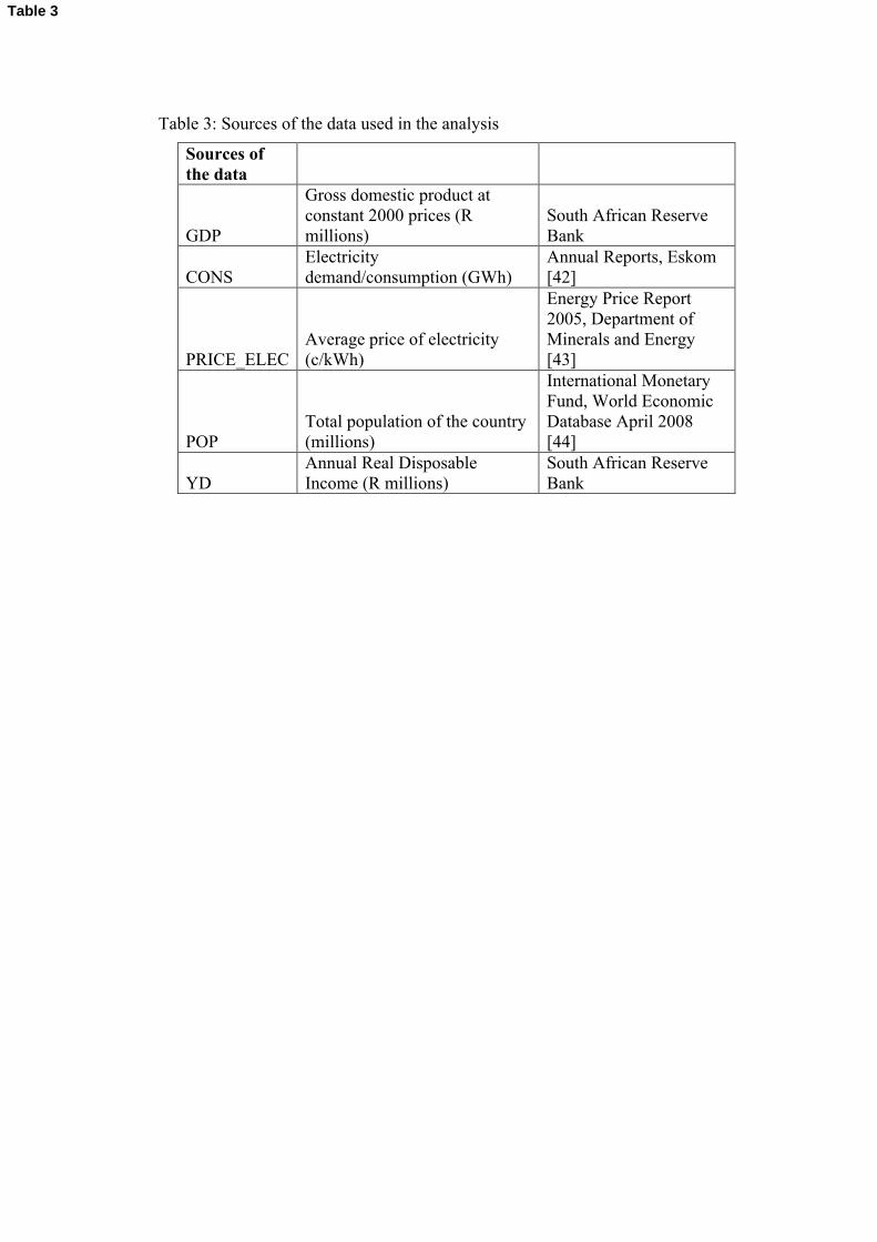
Table 3: Sources of the data used in the analysis

Sources of the data

GDP

Gross domestic product at constant 2000 prices (R millions)

South African Reserve Bank

CONSElectricity demand/consumption (GWh)

Annual Reports, Eskom[42]

PRICE_ELECAverage price of electricity (c/kWh)

Energy Price Report 2005, Department of Minerals and Energy[43]

POPTotal population of the country (millions)

International Monetary Fund, World Economic Database April 2008[44]

YDAnnual Real Disposable Income (R millions)

South African Reserve Bank

Table 3

Table 4: Units of Measurement of the Variables

Variables Units

LCONS GWh

LPRICE_ELEC R/KW

LRYD R millions

LGDP R millions

LPOP millions

Table 4

Table 5: Results of ADF and PP tests for stationarity

ADF test PP test Conclusion

series model lags ττ,τμ,τ φ3,φ1 lags PP

lcons trend 1-

1.326429 1.85212 2 -1.38291

constant 0-

2.660136 * 7.07632 *** 2 -3.83862 ***

none 0 6.642222 - 2 6.642222non stationary

d(lcons) trend 0-

4.312523 ** 9.30194 *** 2 -4.44788 ***

constant 0-

3.863324 *** 14.92527 *** 2 -3.84727 ***

none 0-

2.339497 ** - 2 -2.2713 ** stationary

lprice_elec trend 5 -2.44206 3.35458 0 -2.47191constant 5 -3.13889 ** 2.97591 0 -0.00396

none 0 2.034845 - 0 1.945599non stationary

d(lprice_elec) trend 0-

4.309595 ** 9.28987 *** 2 -4.32494 **

constant 0-

4.239398 *** 17.97249 *** 2 -4.2394 ***

none 2-

1.792374 * - 2 -3.82973 *** stationary

lryd trend 2-

0.370021 3.04745 0 -1.07239constant 2 2.184813 4.07182 0 7.7526

none 2 4.502431 - 0 6.454969non stationary

d(lryd) trend 1 -5.76316 *** 11.78629 *** 2 -7.20009 ***

constant 1-

4.838414 *** 12.56828 *** 2 -4.03303 ***

none 3-

0.029597 - 2 -1.81266 * stationary

lgdp trend 1-

0.640349 3.12373 0 0.085266constant 2 2.205639 2.81091 0 3.170404

none 1 2.471243 - 0 4.58334non stationary

d(lgdp) trend 1-

3.908287 ** 6.03028 *** 2 -4.91042 ***

constant 1-

2.831978 * 5.09085 2 -3.71095 **

none 0-

2.534926 ** - 2 -2.53493 ** stationary

Table 5

Table 6 Engle Granger co-integration results

Variable Model Lags τRes_coint None 0 -3.917576

Table 6

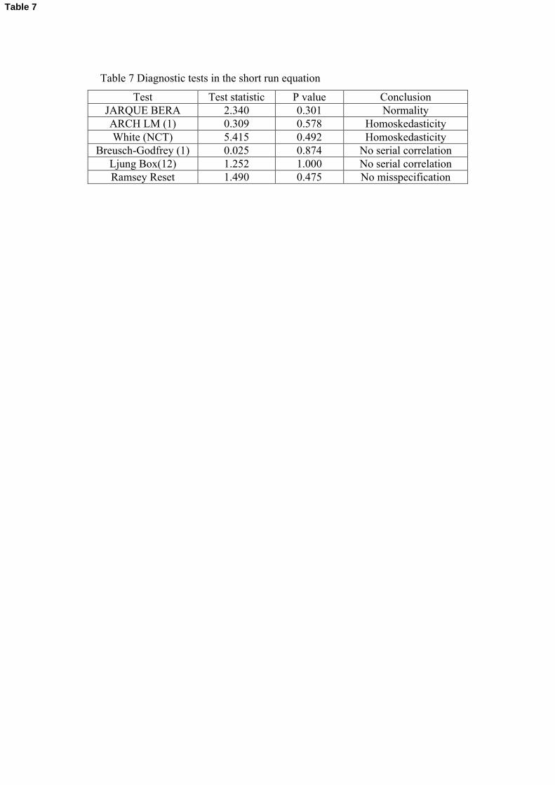
Table 7 Diagnostic tests in the short run equation

Test Test statistic P value ConclusionJARQUE BERA 2.340 0.301 NormalityARCH LM (1) 0.309 0.578 HomoskedasticityWhite (NCT) 5.415 0.492 Homoskedasticity

Breusch-Godfrey (1) 0.025 0.874 No serial correlationLjung Box(12) 1.252 1.000 No serial correlationRamsey Reset 1.490 0.475 No misspecification

Table 7

1

Table 8: Engle Yoo adjustment

Variables Adjusted coefficientsLPRICE_ELEC -0.564388+0.011883=-0.552505LRYD 0.415060+0.002591=0.417651

Table 8