1 Adaptive error estimation of the Trefftz method for solving the Cauchy problem Presenter: C.-T....

1

Adaptive error estimation of the Trefftz method for solving the Cauchy problem

Presenter: C.-T. Chen

Co-author: K.-H. Chen, J.-F. Lee & J.-T. Chen

BEM/MRM 29, 4-6 June 2007, The New Forest, UK

2

Trefftz method for interior problems

Statement of problem

Numerical example

Conclusions

Motivation

Regularization techniques

Outlines

3



Numerical example

Conclusions

Motivation


Outlines

4

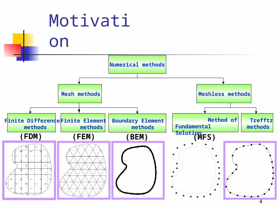
Numerical methods

Motivation

Mesh methods

Finite Difference methods

Finite Element methods

Boundary Element methods

Meshless methods

Trefftz methods

Method of Fundamental Solution (MFS)(FDM) (FEM) (BEM)

5



Numerical example

Conclusions

Motivation


Outlines

6

Statement of problem Inverse problems (Kubo) :

1. Lake of the determination of the domain, its boundary, or an unknown inner boundary.

2. Lake of inference of the governing equation.

3. Lake of identification of boundary conditions and/or initial conditions.

4. Lake of determination of the material properties involved.

5. Lake of determination of the forces acting in the domain.

Cauchy problem

7

2 ( ) 0,

u x x D

over-specified condition

1 11

1 1

u ( ) = f ( )B :

t ( ) = g ( )

x x

x x

1 2B = B B

D

22

2

u ( ) = ?

t ( ) =:

?B

x

x

2 ( ) 0,

u x x D

D

1 2B = B B

22

2

u ( ) = ?

t ( ) =:

?B

x

x

1 1

11

u ( ) = f ( )B :

t ( ) = ?x

x x

2 ( ) 0,

u x x D

D

1 2B = B B

22

2

u ( ) = ?

t ( ) =:

?B

x

x

11

1

u ( ) = ?

t ( ) =:

?B

x

x

2 ( ) 0,

u x x D

D

1 2B = B B

22

2

u ( ) = ?

t ( ) =:

?B

x

x

1

11

1

B :t ( ) = g

u ( ) = ?

( )x

x x

Lake of identification of boundary conditions and/or initial conditions.

case 1 case 2

case 3 case 4

8



Numerical example

Conclusions

Motivation


Outlines

9

Field solution :

where 2N the number of complete functions

jw the unknown coefficient

( )jA x

the T-complete function which satisfies

the Laplace equation

Trefftz method2

1( )( ) j

N

jju x w A x

10

1

1 10 ( , ) () ,, )( n

N N

nn n

nnF Ga bu a

T-complete set functions :

T-complete set

Where: ( , ) cos( )nnF n ( , ) sin( )n

nG n

( ) 1 cos( ) sin( ), =1,, , 2, n njA x n n n

Field solution :

0 j n nw a a b , , The unknown coefficient :

11

Normal differential of the boundary solution

*1

1

*

1

( , )( , ) ( , )( , )

N N

n nx

nn n nat F bu

nG

1 11

1 1

* sincos( ) cos sin(( , ) )

N Nn n

n xn n

F n n n n nr

1 11

1 1

coscos( ) sin sin( )

N Nn n

yn nn n n n n

r

1

1 1

* sinsin( ) cos c( , ) os( )

N Nn n

xn n

nG n n n n nr

1

1 1

cossin( ) sin cos( ) .

N Nn n

yn nn n n n n

r

where

12



Numerical example

Conclusions

Motivation


Outlines

13

Tikhonov technique

(I)

(II)

2x 2

bAxMinimize

subject to

The proposed problem is equivalent to Minimize

2bAx subject to *

2 x

The Euler-Lagrange equation can be obtained as

bAxIAA TT )(

Where λ is the regularization parameter (Lagrange parameter).

14

The minimization principle xHxb-xAxQxP

2 ][][

in vector notation,

bAxHAA TT )( where

M M M (M-1) (M-1) MH B B

1 -1 0 0 0 0 0 0

-1 2 -1 0 0 0 0 0

0 -1 2 -1 0 0 0 0

0 0 0 0 -1 2 -1 0

0 0 0 0 0 -1 2 -1

0 0 0 0 0 0 -1 1

T

in which

11-000000

011-00000

0000011-0

00000011-

B M1)-(M

Linear regularization method

2[ ]P x A x b where [ ]Q x x H x

15

2 ( ) 0,

u x x D


x x

x x

1 11

1 1

u ( ) = f ( )B :

t ( ) = g ( )

1 2B = B B

D

22

2

u ( ) = ?

t ( ) =:

?B

x

x

The concept of adaptive error estimation

Step 1:

16

1 2B = B B

D

22

2

u ( ) = ?

t ( ) ==

?B

x

x

2 ( ) = 0,

u x x D

The ill-posed problem

Obtain:

Step 2:

2 2 2 2u ( ) = f ( ), t ( ) = g ( )x x x x

x x

x x

1 11

1 1

u ( ) = f ( )B :

t ( ) = g ( )

By Trefftz method

17

1

11

1

B :t ( ) = g

u ( ) = ?

( )x

x x

1 2B = B B

D

22 2u ( )B : = f ( )x x

2 ( ) = 0,

u x x D

Obtain: 1 1u ( ) = f ( )x x

Step 3:

The well-posed problem

18

The optimal parameterNorm

The solution is more sensitive

The system is distorted

The optimal2

2 2 1Norm : dB 2 2 ufuf2

1 1 1Norm : dB 1 1 ffff

1 : Boundary conditionf 2 : Analytical solutionu

19

Flow chart of adaptive error estimation2. . : ( ) 0,

. . : , ,

G E u x x D

BC

1 1 1 1u ( ) f ( ) t ( ) = g ( )

x x x x x B

2 2u ( ) = f ( )x x

Remedied by the Tikhonov technique Remedied by the Linear Regularization Method

, , Let 2 12 1u ( ) t ( ) = g ( )= f ( ) x x x xx B

1 1u ( ) = f ( )x x

Obtain the left value of the boundary Obtain left the value of the boundary

Obtain the right value of the boundary Obtain the right value of the boundary

obtain the optimal Lamda value obtain the optimal Lamda value T L

End

2 2u ( ) = f ( )x x

2

1: dB 1 11 1f ff fNorm error

1 1u ( ) = f ( )x x

, , Let 2 12 1u ( ) t ( ) = g ( )= f ( ) x x x xx B

2

1: dB 1 11 1f ff fNorm error

Trefftz method

Trefftz method

Trefftz method

Trefftz method

20



Numerical example

Conclusions

Motivation


Outlines

21


11

1

( ) sin

( ) sin

u x RB

t x

22

2

( ) ?

( ) ?

u xB

t x

2 u( ) 0, x x D

D

Numerical example

‧

R

Circle case:

22

Analytical field solution : ( ) sin , 0 1u x

-0.8 -0.6 -0.4 -0.2 0 0.2 0.4 0.6 0.8-1

-0.8

-0.6

-0.4

-0.2

0

0.2

0.4

0.6

0.8

23

Inverse Problem with artificial Contamination


11

1

( ) sin [1 ]

( ) sin

(1%)ranu x RB

t x

22

2

( ) ?

( ) ?

u xB

t x

2 u( ) 0,x x D

D

‧R

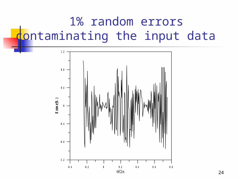
24

1% random errors contaminating the input data

-0.4 -0.2 0 0.2 0.4 0.6 0.8

-1.2

-0.8

-0.4

0

0.4

0.8

1.2

Err

or(

%)

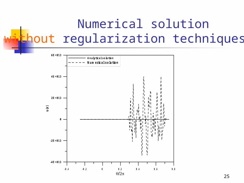
25

Numerical solution without regularization techniques

-0.4 -0.2 0 0.2 0.4 0.6 0.8

-4E+013

-2E+013

0

2E+013

4E+013

6E+013

u(x

)

Analytical solution

Num erical solution

26

Numerical field solution without regularization techniques

-1 -0.8 -0.6 -0.4 -0.2 0 0.2 0.4 0.6 0.8 1-1

-0.8

-0.6

-0.4

-0.2

0

0.2

0.4

0.6

0.8

1

27

Numerical solutions remedied by 3 different (200 nodes)

( )T TA A I x A b ( H)T TA A x A b

-0.4 -0.2 0 0.2 0.4 0.6 0.8

- 2

0

2

u(x

)

The T ikhonov techn ique(200 nodes)Analytical solution

Num erical solution:

Num erical solution: O p t


-0.4 -0.2 0 0.2 0.4 0.6 0.8

- 2

0

2

4

u(x

)

The L inear Regu larization M ethod(200 nodes)Analytical solution


Num erical solution: O p t


28

(T) 0.0000169

-0.8 -0.6 -0.4 -0.2 0 0.2 0.4 0.6 0.8-0.8

-0.6

-0.4

-0.2

0

0.2

0.4

0.6

0.8

-0.8 -0.6 -0.4 -0.2 0 0.2 0.4 0.6 0.8-0.8

-0.6

-0.4

-0.2

0

0.2

0.4

0.6

0.8

-0.8 -0.6 -0.4 -0.2 0 0.2 0.4 0.6 0.8-0.8

-0.6

-0.4

-0.2

0

0.2

0.4

0.6

0.8

Numerical field solutions remedied by the Tikhonov technique with 3 different

(T)Opt 0.00169 (T) 0.169

(200 nodes)

29

-0.8 -0.6 -0.4 -0.2 0 0.2 0.4 0.6 0.8-0.8

-0.6

-0.4

-0.2

0

0.2

0.4

0.6

0.8

-0.8 -0.6 -0.4 -0.2 0 0.2 0.4 0.6 0.8-0.8

-0.6

-0.4

-0.2

0

0.2

0.4

0.6

0.8

-0.8 -0.6 -0.4 -0.2 0 0.2 0.4 0.6 0.8-0.8

-0.6

-0.4

-0.2

0

0.2

0.4

0.6

0.8

(L) 0.0000049 (L) 0.049 (L)Opt 0.00049

Numerical field solutions remedied by the linear regularization method with 3 different

(200 nodes)

30

Obtain the optimal parameters by computing

the Norm deriving from comparing numerical solution with analytic solution

1E-010 1E-007 0.0001 0.1 100

1E-006

1E-005

0.0001

0.001

0.01

0.1

1

10

100

1000

10000

100000

1000000

10000000

100000000

1000000000

No

rm

The Tikhonov techniqueNorm with com paring analytical solution

O p t=0.00169

1E-010 1E-007 0.0001 0.1 100

1E-006

1E-005

0.0001

0.001

0.01

0.1

1

10

100

1000

10000

100000

1000000

10000000

No

rm

The Linear Regularization MethodNorm with com paring analytical solution

O p t=0.000499

2

2 2 1Norm : dB 2 2 ufuf 2 : Analytical solutionu

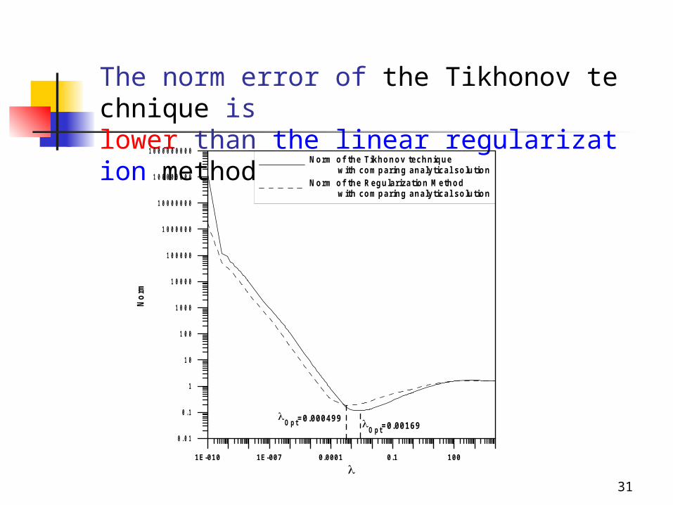
31

The norm error of the Tikhonov technique is lower than the linear regularization method

1E-010 1E-007 0.0001 0.1 100

0.01

0.1

1

10

100

1000

10000

100000

1000000

10000000

100000000

1000000000N

orm

Norm of the Tikhonov technique with com paring analytical solutionNorm of the Regularization Method with com paring analytical solution

O p t=0.00169O p t=0.000499

32

The Tikhonov technique and the Linear Regularization Method

-0.4 -0.2 0 0.2 0.4 0.6 0.8

- 2

- 1

0

1

2u

(x)

O p tT =0.00169 ,O p t

L =0.00049 (200 nodes)

Analytical solutionNum erical solution of the Tikhonov techniqueNum erical solution of the Linear Regularization Method

Numerical solutions with optimal (200 nodes)

33

Numerical field solutions with optimal (200 nodes)

The Tikhonov technique The Linear Regularization Method

-0.8 -0.6 -0.4 -0.2 0 0.2 0.4 0.6 0.8-0.8

-0.6

-0.4

-0.2

0

0.2

0.4

0.6

0.8

-0.8 -0.6 -0.4 -0.2 0 0.2 0.4 0.6 0.8-0.8

-0.6

-0.4

-0.2

0

0.2

0.4

0.6

0.8

(T)Opt 0.00169 (L)

Opt 0.00049

34

Under no exact solution, the optimal results obtained by using the adaptive error estimation

1E-010 1E-007 0.0001 0.1 100

1E-006

1E-005

0.0001

0.001

0.01

0.1

1

10

100

1000

10000

100000

1000000

10000000

100000000

1000000000

No

rm

The Tikhonov techniqueNorm with com paring analytical solutionNorm with adaptive error estim ation

O p t=0.00169

O p t=0.00409

1E-010 1E-007 0.0001 0.1 100

1E-006

1E-005

0.0001

0.001

0.01

0.1

1

10

100

1000

10000

100000

1000000

10000000

No

rm

The L inear Regu larization M ethodNorm with com paring analytical solutionNorm with adaptive error estim ation

O p t=0.000499

O p t=0.000899

The Tikhonov technique The Linear Regularization Method

35



Numerical exampleConclusions

Motivation


Outlines

36

1. The optimal parameters make the system insensitive to contaminating noise.

2. The present results were well compared with exact solutions.

3. The Tikhonov technique agreed the analytical solution better than another in this example.

4. Under no exact solution, the optimal results are obtained by employing the adaptive error estimation.

Conclusions

37

Thanks for your attentions.

Your comment is much appreciated.

38

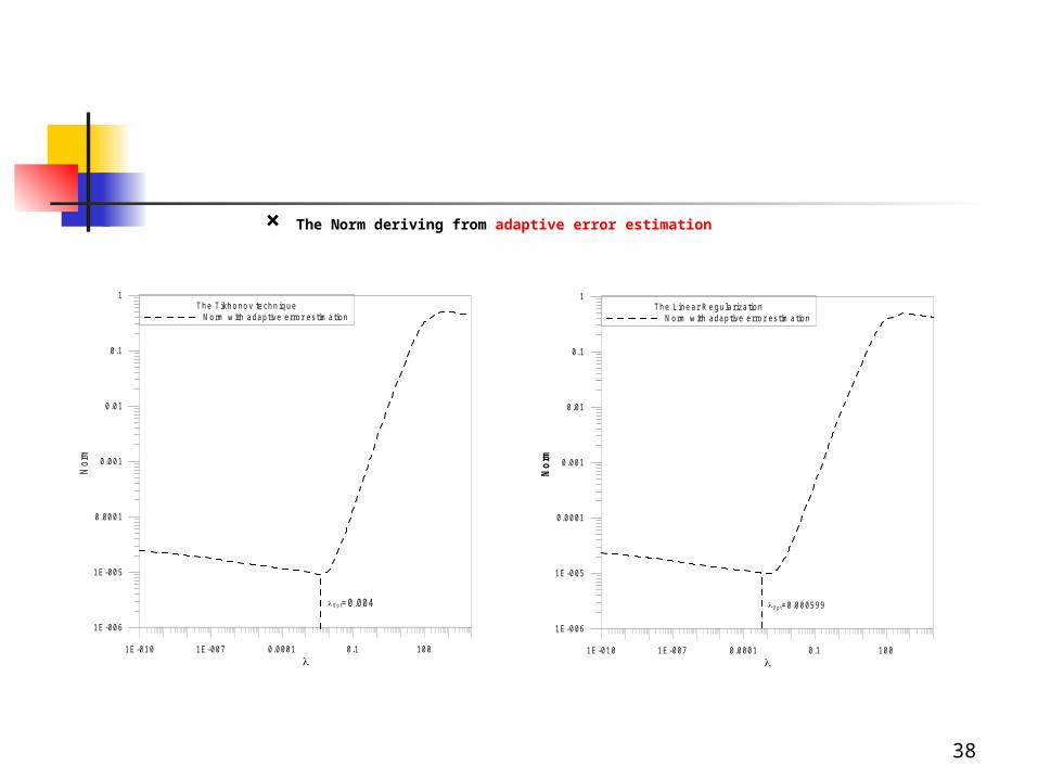
× The Norm deriving from adaptive error estimation

1E-010 1E-007 0.0001 0.1 100

1E-006

1E-005

0.0001

0.001

0.01

0.1

1

No

rm

Th e L in e a r R e g u la riza tio nN orm w ith adaptive error estim ation

O p t=0.000599

1E-010 1E-007 0.0001 0.1 100

1E-006

1E-005

0.0001

0.001

0.01

0.1

1

Nor

m

Th e Tikh o n o v te ch n iq u eN orm w ith adaptive error estim ation

O p t=0.004

39

-0 .8 -0.6 -0.4 -0.2 0 0.2 0.4 0.6 0.8-0.8

-0.6

-0.4

-0.2

0

0.2

0.4

0.6

0.8

-0.8 -0.6 -0.4 -0.2 0 0.2 0.4 0.6 0.8-0.8

-0.6

-0.4

-0.2

0

0.2

0.4

0.6

0.8

0.0002 0.02 Opt 0.002

-0.8 -0.6 -0.4 -0.2 0 0.2 0.4 0.6 0.8-0.8

-0.6

-0.4

-0.2

0

0.2

0.4

0.6

0.8

Figure 9(a) The numerical field solution remedied by the Tikhonov technique with 3 different lambdas (200nodes)

40

Numerical solution being remedied by the Linear Regularization Method with 3 different lambdaes(200 nodes)

0.000049

-1 -0.8 -0.6 -0.4 -0.2 0 0.2 0.4 0.6 0.8 1-1

-0.8

-0.6

-0.4

-0.2

0

0.2

0.4

0.6

0.8

1

Opt 0.00049

-1 -0.8 -0.6 -0.4 -0.2 0 0.2 0.4 0.6 0.8 1-1

-0.8

-0.6

-0.4

-0.2

0

0.2

0.4

0.6

0.8

1

0.0049

-1 -0.8 -0.6 -0.4 -0.2 0 0.2 0.4 0.6 0.8 1-1

-0.8

-0.6

-0.4

-0.2

0

0.2

0.4

0.6

0.8

1

Figure 9(b) The numerical field solution remedied by the linear regularization method with 3 different lambdas (200nodes)

41

-0.8 -0.6 -0.4 -0.2 0 0.2 0.4 0.6 0.8-0.8

-0.6

-0.4

-0.2

0

0.2

0.4

0.6

0.8

-0 .8 -0.6 -0.4 -0.2 0 0.2 0.4 0.6 0.8-0.8

-0.6

-0.4

-0.2

0

0.2

0.4

0.6

0.8

Opt 0.002

×Figure 14 (a), 14(b) Numerical field solution being remedied by the Tikhonov technique and the linear regularization method with optimal lambda (200 nodes)

Opt 0.00049 The Tikhonov technique: The Linear Regularization Method:

42

-0 .4 -0.2 0 0.2 0.4 0.6 0.8

- 2

- 1

0

1

2

u(x)

Th e Tikh o n o v M e th o dAnalytic S olu tion

N um erica l so lu tion(40 nodes)


Numerical solution being remedied by the Tikhonov technique Of 40 nodes and 200 nodes with optimal lambda

43

Numerical solution being remedied by the Linear Regularization Method Of 40 nodes and 200 nodes with optimal lambda

-0 .4 -0.2 0 0.2 0.4 0.6 0.8

- 2

- 1

0

1

2u(x)

Th e L in e a r R e g u la riza tio n M e th o dAnalytic S olu tion



1 Adaptive error estimation of the Trefftz method for solving the Cauchy problem Presenter: C.-T....

Documents

Transcript of 1 Adaptive error estimation of the Trefftz method for solving the Cauchy problem Presenter: C.-T....