1

A Tube-and-Droplet-based Approach forRepresenting and Analyzing Motion Trajectories

Weiyao Lin, Yang Zhou, Hongteng Xu, Junchi Yan, Mingliang Xu, Jianxin Wu, and Zicheng Liu

F

Abstract—Trajectory analysis is essential in many applications. In thispaper, we address the problem of representing motion trajectories in ahighly informative way, and consequently utilize it for analyzing trajecto-ries. Our approach first leverages the complete information from giventrajectories to construct a thermal transfer field which provides a context-rich way to describe the global motion pattern in a scene. Then, a 3Dtube is derived which depicts an input trajectory by integrating its sur-rounding motion patterns contained in the thermal transfer field. The 3Dtube effectively: 1) maintains the movement information of a trajectory,2) embeds the complete contextual motion pattern around a trajectory,3) visualizes information about a trajectory in a clear and unified way.We further introduce a droplet-based process. It derives a droplet vectorfrom a 3D tube, so as to characterize the high-dimensional 3D tubeinformation in a simple but effective way. Finally, we apply our tube-and-droplet representation to trajectory analysis applications includingtrajectory clustering, trajectory classification & abnormality detection,and 3D action recognition. Experimental comparisons with state-of-the-art algorithms demonstrate the effectiveness of our approach.

1 INTRODUCTION

MOTION information, which reflects the temporal vari-ation of visual contents, is essential in depicting the

semantic contents in videos. As the motion information ofmany semantic contents is described by motion trajectories,trajectory analysis is of considerable importance to manyapplications including video surveillance, object behavioranalysis, and video retrieval [1]–[5]. Formally, trajectoryanalysis can be defined as the problem of deciding the classof one or more input trajectories according to their shapesand motion routes [4], [6]–[8].

A motion trajectory is in general obtained by trackingan object over frames and linking object positions into aposition sequence [1], [2], [9]. Although trajectories containdetailed information of object movements, reliable trajectoryanalysis remains challenging due to the uncertain nature

• W. Lin and Y. Zhou are with the Dept. of Electronic Engineer-ing, Shanghai Jiao Tong University, Shanghai, China. E-mail: {wylin,zhz128ly}@sjtu.edu.cn.

• H. Xu is with the Dept. of Electrical and Computer Engineering, GeorgiaInstitute of Technology, Atlanta, USA. E-mail: hxu42@gatech.edu.

• J. Yan is with IBM Research, Shanghai, China. E-mail: yanjc@cn.ibm.com.• M. Xu is with Zhengzhou University, Zhengzhou, China. E-mail: iex-

umingliang@zzu.edu.cn.• J. Wu is with the National Key Laboratory for Novel Software Technology,

Nanjing University, Nanjing, China. E-mail: wujx2001@nju.edu.cn.• Z. Liu is with Microsoft Research, Redmond, USA. E-mail:

zliu@microsoft.com.

(a) (b) (c)

Figure 1. (a) An example of ambiguous trajectories: The orange, red,and green curves labeled by CP1-CP3 indicate three trajectory classes.The black curves labeled by Trajectory A andB are two trajectories fromCP1 and CP2, respectively. (b) Complete contextual motion patterns oftrajectories A and B in (a): Contextual motion patterns are describedby the motion flows of all trajectory points in the neighborhood of Aand B (Note: We use color to differentiate motion flows from differenttrajectory classes only for a clearer illustration. In our approach, we donot differentiate motion flows’ classes and directly use all motion flowsin the neighborhood of an input trajectory to model its contextual motionpattern). (c) Use our 3D tube to model A and B’s complete contextualmotion patterns. (Best viewed in color)

of object motion and the ambiguity from similar motionpatterns.

One major challenge for trajectory analysis is to differ-entiate trajectory classes with only subtle differences. Forexample, Fig. 1a shows three trajectory classes CP1, CP2,and CP3, where CP1 and CP2 include vehicle trajectoriesfollowing two adjacent leftward street lanes and CP3 in-cludes vehicle trajectories following a left-turn street lane.Since trajectories in CP1 and CP2 are similar in both motiondirection and location, the original position sequence repre-sentation is insufficient to differentiate them. This necessi-tates the development of more informative motion trajec-tory representation. However, most existing trajectory rep-resentation methods [3], [4], [10], [11] focus on performingtransformation or parameterization on the original positionsequence, while the problem of more informative repre-sentation is not well addressed. Although some trajectory-modeling or local-modeling methods [4], [6], [7], [12], [13]increase the informativeness of trajectories by including thecontextual information among multiple trajectories, theyonly model partial contextual information from trajectorieswith similar patterns or trajectories in the same class. Thus,they still have limitations when differentiating ambiguoustrajectories, such as trajectories near the boundary of similartrajectory classes (e.g., trajectories A and B in Fig. 1a).

We argue that due to the stable constraint from a scene,the complete contextual motion pattern around a trajectoryprovides an important cue for trajectory depiction. By com-

2

Figure 2. The framework of the proposed approach. It constructs a scene-specific thermal transfer field via trajectory training data; For a testtrajectory sample, it builds a 3D tube based on the constructed thermal transfer field, and generates a feature vector via a droplet process. Theobtained feature vector is applicable to various trajectory analysis applications. (Best viewed in color)

plete, we refer to the contextual motion information from allgiven trajectories in the neighborhood of an input trajectory.For example, Fig. 1b shows the complete contextual motionpatterns of two easily-confused trajectories A and B whichare extracted from two similar trajectory classes CP1 andCP2. If we look at the contextual motion information inthe neighborhood of trajectory A, there is a strong left andslightly upward motion pattern (in green color) towards theend of A. In contrast, if we look at the contextual motioninformation in the neighborhood of trajectory B, there is anobvious upward motion pattern in the middle of B. Thus,the ambiguity between trajectories is expected to be reducedif the above-mentioned contextual motion information isproperly modeled (cf. Fig. 1c).

1.1 Our Work

Based on this intuition, we develop a novel frameworkwhich utilizes the global motion trends in a scene to describea trajectory. Specifically, for each point in a trajectory, wederive the dominant scene motion pattern around the pointand utilize it to depict the point’s complete contextualmotion pattern. By integrating the dominant scene motionpatterns for all points in a trajectory, we are able to describea trajectory in a highly informative way and make finedistinctions among similar trajectories. The framework ofour approach is shown in Fig. 2.

Given a set of trajectories, thermal transfer fields are firstconstructed to describe the global motion pattern in thescene (cf. module ‘constructing thermal transfer fields’ inFig. 2). Then, for an input trajectory, we expand it over thetime domain to construct a 3D spatio-temporal curve, andderive an equipotential line for each point in this curve (cf.module ‘deriving equipotential lines’ in Fig. 2). The equipo-tential lines are decided by the locations of spatio-temporalcurve points and their surrounding dominant scene motionpatterns defined in thermal transfer fields. In this way, thecomplete contextual motion pattern can be captured.

After obtaining equipotential lines, a 3D tube is con-structed which concatenates equipotential lines accordingto the temporal order of spatio-temporal curve points (cf.module ‘constructing 3D tubes’ in Fig. 2). This 3D tube isable to depict an input trajectory in a highly informativeway, where the movement of a trajectory and the contextualmotion pattern around a trajectory are effectively capturedby the route and shape of the 3D tube.

Finally, a droplet-based process is applied which ‘injects’water in one end of a 3D tube and achieves a water dropletflowed out from the other end. This water droplet is furthersampled to achieve a low-dimensional droplet vector tocharacterize the 3D tube shape (cf. module ‘droplet-basedprocess for feature extraction’ in Fig. 2). Since differenttrajectories are depicted by 3D tubes with different shapes,by suitably modeling the water flow process, the dropletvector can precisely catch the unique characteristics of a 3Dtube. The droplet vector will serve as the final trajectoryrepresentation format and is applied in trajectory analysis.

In summary, our contributions are three folds.• We construct a thermal transfer field to describe the

global motion pattern in a scene, derive equipotentiallines to capture the contextual motion information of tra-jectory points, and introduce a 3D tube by concatenatingequipotential lines to represent a motion trajectory. Thesecomponents establish a novel framework for addressingthe informative trajectory representation problem.• Under this framework, we develop a droplet-based

process which derives a simple but effective low-dimensional droplet vector to characterize the high-dimensional information in a 3D tube. The deriveddroplet vector can not only capture the characteristicsof a 3D tube, but also suitably reduce the disturbancefrom trajectory noises.• We investigate our tube-and-droplet representation to

various trajectory analysis applications including trajec-tory clustering, trajectory classification & abnormalitydetection, and 3D action recognition, and achieve thestate-of-the-art performance.

2 RELATED WORKS

2.1 Trajectory Representation and Modeling

Properly representing motion trajectories is crucial to tra-jectory analysis. Many algorithms [1], [5], [6], [9], [14] havebeen proposed for trajectory representation. Most of them[3], [10], [11], [14] aim to find suitable parameter setsto describe trajectories. Discrete Fourier transform (DFT)coefficients [10] and polynomial curve fitting [3] are twoexamples. Rao et al. [14] extracted dynamic instants andused them as the key points to represent the spatio-temporalcurvature of trajectories. These methods focus more on theeffective representation of a trajectory’s position sequence,

3

while the issue of more informative representation is not ad-dressed. Although some works [1]–[3], [12], [14] increase theinformativeness of trajectory representation by introducingadditional information such as motion velocity, temporalorder, or object size, the added information is still restrictedwithin a single trajectory and cannot be used to discriminatetrajectories with similar patterns.

Trajectory-modeling methods that include the contextualinformation of multiple trajectories are also proposed [4],[6], [7]. These methods construct probability models foreach trajectory class and utilize them to guide the trajec-tory analysis process. Kim et al. [6] introduced Gaussianprocess regression flows to model the location and velocityprobability for each trajectory class. Morris and Trivedi [7]clustered trajectories into spatial routes and encoded thespatio-temporal dynamics of each cluster by hidden Markovmodels (HMM). Hu et al. [4] built a time-sensitive Dirichletprocess mixture model (tDPMM) to represent the spatio-temporal characteristics of each trajectory class. These meth-ods only focus on modeling the contextual information in-side each individual class, while ignoring information fromexternal trajectory classes. Therefore, they still have limita-tions when differentiating ambiguous trajectories, such astrajectories near the boundary of similar trajectory classes.

Another line to integrate contextual information is thelocal-modeling methods [13], [15]. These methods aim toutilize dynamic models or topic models to describe trajec-tories’ local motion patterns. Nascimento et al. [15] intro-duced low-level dynamic models to decompose trajectoriesinto basic displacement patterns, and recognized trajectoriesbased on the switch among these low-level models. Wanget al. [13] proposed a non-parametric topic model calledDual Hierarchical Dirichlet Processes (Dual-HDP), whichconstructs local semantic regions including similar trajec-tory segments and performs trajectory analysis accordingly.Although these models share the contextual informationfrom multiple trajectory classes, only the contextual in-formation from similar trajectory segments is considered.Therefore, they are less effective when trajectories have largevariations or reliable local models cannot be constructed dueto insufficient similar trajectory segments.

The proposed 3D tube representation differs with exist-ing approaches in the following aspects:

• We model the complete contextual information arounda trajectory, not only the contextual information frompartial trajectories. This enables us to precisely catch thesubtle changes among different trajectory classes.• Most existing works handle trajectory analysis with

complex probability models, which require sufficienttrajectory data to construct reliable models. We establisha novel framework to model trajectories in a simplebut effective way, which can work robustly under rela-tively small data size. Experimental evaluation shows wecan achieve state-of-the-art performance on benchmarkdatasets with this simple procedure.• Existing methods focus on the abstract modeling of

trajectory information where the modeled trajectory in-formation cannot be easily visualized. Our 3D tube rep-resentation is able to visualize a variety of trajectory in-formation, including spatial-temporal movements, con-

textual motion patterns, and possible motion directions,in a clear and unified way.

2.2 Handling High-Dimensional Representations

Since highly informative trajectory representation oftenleads to a complex and high-dimensional representationformat, it is non-trivial to find suitable ways to handle thishigh-dimensional representation for trajectory analysis.

In [16], Euclidean distance and dynamic time wrapping(DTW) distance were utilized to measure the distance of twotime-series trajectory sequences. Vlachos et al. [17] furtherintroduced the longest common subsequence (LCSS) dis-tance. While these methods can handle the original positionsequence format of a trajectory, they are not suitable toprocess higher dimensional representations.

In order to handle higher-dimensional data represen-tations, some dimension reduction approaches were de-veloped [18], [19]. However, due to the large variationand ambiguity among trajectories, trajectory representationsoften have complex distributions. Thus, simply applyingdimension reduction cannot achieve satisfactory results.Moreover, some advanced manifold approaches were alsointroduced [20]–[22]. In [20], Lui modeled high-dimensionalinputs as high-order tensors. The similarity between inputswere measured by the intrinsic distance between tensors,which is estimated through manifold charting. Althoughthese methods can achieve better results when process-ing high-dimensional trajectory representations, they haveconsiderably high computation complexity. Thus they aredifficult to be applied on large scale trajectory analysis.

Besides dimension reduction, other works [12], [23], [24]aim to develop proper distance metrics to measure thesimilarity between high-dimensional inputs. Lin et al. [12]introduced a surface matching distance to measure the sim-ilarity between high-dimensional surface shapes. Sangineto[23] and Gao et al. [24] developed advanced Hausdorffdistance which treats each high-dimensional input as a set ofpoints and estimates the similarity between inputs from thedistance between point sets. These methods are dependenton the quality of high-dimensional inputs, and noisy inputswill adversely affect the performance of these methods.

Different from the previous methods, we develop a noveldroplet-based process which simulates the physical waterflow process and derives a low-dimensional droplet vectorto characterize the high-dimensional 3D tube shape. Thisprocess has low complexity and can suitably reduce thedisturbance from trajectory noises.

3 3D TUBE REPRESENTATION

In order to include the complete contextual motion informa-tion in trajectory representation, it is important to properlymodel and embed the global motion pattern information ina scene. More specifically, assuming that there are M tra-jectories available from a scene, denoted as {Γm}Mm=1. Eachtrajectory is represented as Γm = {pmn }L

m

n=1, where pmn ∈ R2

is the position of the nth point of the trajectory and Lm is thelength of trajectory Γm. Accordingly, the speed of the point inthe position is calculated as umn =

pmn+1−p

mn

∆t ∈ R2, where ∆tis the sampling interval between adjacent points. We aim to

4

find the scene’s global motion pattern which best describesthe motion trends provided by M given trajectories1, anduse this global motion pattern to derive the complete con-textual motion patterns for positions along the route of aninput trajectory. In this way, we are able to construct a 3Dtube from these contextual motion patterns and obtain aninformative representation for the input trajectory.

In this paper, we borrow the idea from thermal propaga-tion [25]–[27] and introduce a trajectory model, which findsglobal motion pattern, derives contextual motion patterns,and constructs 3D tube representations with thermal propa-gation processes.

3.1 Constructing Thermal Transfer FieldsFirst, we model the global motion pattern in a scene basedon the works in fluid thermal propagation [25]–[27]. Specif-ically, the aggregation of M given trajectories is modeledas a ‘fluid’ in the scene, where each pmn is a sample of thefluid and the corresponding umn refers to the movement ofthe fluid which results in the transfer of thermal energies inposition pmn .

According to thermal transmission theories [25], [26],the thermal diffusion result of the entire fluid is affectedby a scene-related thermal transfer field which decides thethermal propagation strengths at different positions and indifferent directions. Therefore, by constructing an optimalthermal transfer field that best suits the thermal dynamicsof the fluid defined by given trajectories, the fluid’s thermaldynamics, which characterize the motion pattern from Mgiven trajectories, can be effectively embedded in the ther-mal transfer field.

In this work, we construct a scene’s thermal transferfield based on the strategy of finite-element analysis [27].Formally, we first segment the scene into grids of positionsG = [1, ...,W ] × [1, ...,H], where W and H are the widthand height of the scene. Then, the thermal transfer field ofthe scene can be represented as:

K = [k(p,a)]W×H×|A| (1)

where k(p,a) (p ∈ G, a ∈ A) is the thermal transfer co-efficient indicating the thermal propagation strength alongdirection a at position p. Here a is a normalized vector(‖a‖2 = 1) indicating thermal propagation directions, whichis selected from a pre-defined direction setA. |A| counts thenumber of directions in the set. In this paper,A contains fourdirections, which depicts a scene’s global motion pattern inupward (y−), downward (y+), leftward (x−), and rightward(x+) directions, respectively (cf. module ‘constructing ther-mal transfer fields’ in Fig. 2).

Assuming that the given trajectories correspond to astable fluid, we can construct an optimal thermal transferfield K by minimizing the total amount of thermal energiesbeing transferred during the fluid flow process, as:

minK

∑a∈A

∑p∈G

∆E(k(p,a)) (2)

s.t. k(p,a) ≥ 0,∑p∈G

k(p,a) = κ, for a ∈ A.

1. Note that we do not differentiate given trajectories’ class labels,and directly use all given trajectories to find global motion patterns.

where ∆E(k(p,a)) is the amount of thermal energy trans-ported by the fluid from position p along direction a withina unit time interval. κ (κ > 0) is a constant. The first con-straint in (2) guarantees to achieve physically-meaningfulthermal transfer fields (i.e., avoid negative transfer fields),and the second constraint guarantees to obtain proper dis-tributions of k(p,a) (i.e., avoid transfer fields becoming allinfinite values). ∆E(k(p,a)) can be calculated from thermaltransmission theories [25], [26]:

∆E(k(p,a)) = ηρ(p)u(p,a)

k(p,a)(3)

Here η is a parameter related to the temperature differencebetween a position p and its neighbors [25], [26]. In our pa-per, since we want to focus on the relationship between ∆Eand k(p,a), we simply assume the temperature differencecondition to be the same when calculating ∆E at differentpositions, and set η as a constant. ρ(p) is the density of fluidat position p, u(p,a) is the moving velocity along direction aat position p. Physically, ρ(p)u(p,a) measures the numberof fluid particles passing through position p along directiona within a unit time interval. k(p,a) indicates the efficiencyof thermal energy transfer along direction a at p. As a result,k(p,a)∆E refers to the amount of thermal energies actuallyreceived by p’s neighboring position when an amount ofenergy ∆E is transferred out from p [25], [26].

According to (2) and (3), we let a fluid flow along theaggregated routes of M given trajectories, and measure thetotal amount of thermal energy transfers over all positions.The thermal transfer field that leads to the smallest totaltransferred energy will be the optimal field that best suitsthe scene.

More specifically, from (3), the amount of energy transfer∆E is jointly decided by k(p,a) (thermal transfer coeffi-cient), ρ(p) (fluid’s density), and u(p,a) (fluid’s velocity).When ρ(p)u(p,a) increases, the amount of fluid flowingalong direction a at p becomes stronger, which leads tolarger chances of energy transfer. Thus, by minimizing∑

a,p ∆E in (2), k(p,a) is proportionally adjusted withρ(p)u(p,a) such that k(p,a) with higher energy transfer ef-ficiencies are assigned to positions/directions with strongerfluid flows. In this way, the resulting thermal transfer fieldcan properly suit the thermal dynamics of the fluid.

ρ(p) in (3) is calculated based on the nonparametricestimation of sample points pmn in given trajectories:

ρ(p) =M∑m=1

Lm∑n=1

exp

(−‖p− pmn ‖

2σ2

). (4)

Similarly, u(p,a) in (3) is the nonparametric estimation ofsample points and their corresponding projected speeds:

u(p,a) =M∑m=1

Lm∑n=1

max(a>umn , 0) exp

(−‖p− pmn ‖

2σ2

)(5)

where a>umn is the projection of speed umn in a-th direction.max(a>umn , 0) ensures that only the directions with positivevelocity are considered.

(4) and (5) ensure that ρ(p)u(p,a) can correctly reflectthe global motion pattern contained in given trajectories. Forexample, when a large number of trajectories pass through

5

(a) (b)

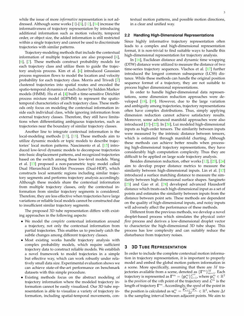
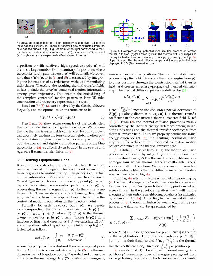
Figure 3. (a) Input trajectories (black solid curves) and given trajectories(blue dashed curves). (b) Thermal transfer fields constructed from theblue dashed curves in (a). Figures from left to right correspond to ther-mal transfer fields in directions upward (y−), downward (y+), leftward(x−), rightward (x+), respectively. (Best viewed in color)

a position p with relatively high speed, ρ(p)u(p,a) willbecome a large number. On the contrary, for positions wheretrajectories rarely pass, ρ(p)u(p,a) will be small. Moreover,note that ρ(p)u(p,a) in (4) and (5) is estimated by integrat-ing the information of all trajectories without differentiatingtheir classes. Therefore, the resulting thermal transfer fieldsin fact include the complete contextual motion informationamong given trajectories. This enables the embedding ofthe complete contextual motion pattern in later 3D tubeconstruction and trajectory representation steps.

Based on (3)-(5), (2) can be solved by the Cauchy–Schwarzinequality and the optimal solutions turns out to be:

k(p,a) ∝√ρ(p)u(p,a) (6)

Figs 2 and 3b show some examples of the constructedthermal transfer fields from given trajectories. We can seethat the thermal transfer fields constructed by our approachcan effectively capture the four-direction global motion pat-terns contained in given trajectories. For example, in Fig. 3,both the upward and rightward motion patterns of the bluetrajectories in (a) are effectively embedded in the upward andrightward thermal transfer fields in (b).

3.2 Deriving Equipotential LinesBased on the constructed thermal transfer field K, we canperform thermal propagation for each point in an inputtrajectory, so as to embed the input trajectory’s contextualmotion information. More specifically, we first obtain athermal diffusion map for an input trajectory point pmn , whichdepicts the dominant scene motion pattern around pmn bypropagating thermal energies from pmn to the entire scenethrough K. Then we derive a constant-energy line calledequipotential line from this map, and use it to capture thecontextual motion information for the trajectory point.

Formally, for each trajectory point pmn , we denoteits corresponding thermal diffusion map as E(pmn ) =[E(pmn ,p)]W×H , p ∈ G, where E(pmn ,p) is the thermalenergy at position p in pmn ’s map. Taking E(pmn ) as afunction of time t and direction a ∈ A, we calculate E(pmn )via an iterative method. Specifically, the initial map E0(pmn )is defined as follows:

E0(pmn ,p) =

{Eε, if p = pmn0, otherwise

, (7)

where E0(pmn ,p) is the initialized thermal energy at posi-tion p. Eε = 100 is a constant. According to (7), the thermaldiffusion map of trajectory point pmn is initialized by assign-ing a large thermal energy to pmn ’s position and assigning

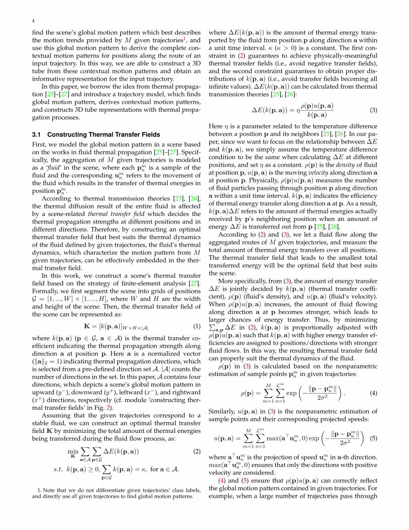
(a) (b) (c) (d)

Figure 4. Examples of equipotential lines. (a) The process of iterativethermal diffusion. (b)-(d) Lower figures: The thermal diffusion maps andthe equipotential lines for trajectory points pa, pb, and pc in Fig. 3a;Upper figures: The thermal diffusion maps and the equipotential linesdisplayed in 3D. (Best viewed in color)

zero energies to other positions. Then, a thermal diffusionprocess is applied which transfers thermal energies from pmnto other positions through the constructed thermal transferfield, and creates an energy-propagated thermal diffusionmap. The thermal diffusion process is defined by [25]:

∂E(pmn ,p)

∂t=∑a∈A

k(p,a)∂2E(pmn ,p)

∂a2. (8)

Here ∂2E(pmn ,p)

∂a2 means the 2nd order partial derivative ofE(pmn ,p) along direction a. k(p,a) is a thermal transfercoefficient in the constructed thermal transfer field K (cf.(1)-(2)). From (8), the thermal diffusion process is mainlycontrolled by the thermal energy difference among neigh-boring positions and the thermal transfer coefficients fromthermal transfer field. Thus, by properly setting the initialenergy difference (cf. (7)), the resulting thermal diffusionmap can effectively capture the desired contextual motionpattern contained in the thermal transfer field.

(8) is difficult to solve because: 1) The thermal diffusionprocess is performed by integrating the information frommultiple directions a; 2) The thermal transfer fields are non-homogeneous whose thermal transfer coefficients k(p,a)vary over different locations. We propose an approximationsolution which obtains thermal diffusion map in an iterativeway, as illustrated in Fig. 4a.

From Fig. 4a, after initializing a thermal diffusion map by(7), the thermal energy at pmn is diffused iteratively outwardto other positions. During each iteration τ , positions whichwere diffused in the previous iteration τ − 1 will diffuseenergies to their outside neighboring positions (as indicatedby arrows in Fig. 4a). According to the thermal diffusionprocess in (8), thermal diffusion between neighboring posi-tions in one iteration can be approximated by:

Eτ (pmn ,p) ≈

∑p′∈B(p)Eτ−1(pmn ,p

′) exp

(− ‖p−p′‖k(p, p−p′

‖p−p′‖ )

)|B(p)|

(9)where B(p) is the neighborhood of p and |B(p)| is the sizeof the neighborhood. For p and its neighbors p′ ∈ B(p),‖p − p′‖ is their distance and k(p, p−p′

‖p−p′‖ ) is the thermal

transfer coefficient along direction p−p′‖p−p′‖ at position p.

(9) reveals that: 1) The diffused thermal energy in aposition p′ is summed over all energies propagated fromits neighboring positions in both vertical and horizontal

6

directions. In this way, the complete contextual informationcan be included. 2) The thermal transfer coefficients k(p,a)control the thermal diffusion results. In this way, the motionpattern information from the thermal transfer field can beproperly reflected in the resulting thermal diffusion map. 3)The thermal diffusion map E(pmn ) for position pmn is fullydecided by the thermal transfer field K (cf. (7) and (9)). Thisimplies that the contextual motion information E(pmn ) foreach position in a scene is fixed after a scene’s global motionpattern K is determined. Therefore, if two input trajectoriespass through position pmn with different routes, they willhave the same thermal diffusion map at pmn .

Fig. 4 shows some examples of thermal diffusion mapresults derived from the thermal transfer fields in Fig. 3b.In Fig. 4, (b)-(d) show the thermal diffusion maps of threepoints pa, pb, pc on the black trajectory A in Fig. 3a.

According to Fig. 3a, since moving rightward frompa appears frequently in the scene (as there are lots ofdashed blue trajectories moving rightward around pa), largerightward-direction thermal transfer coefficients are obtainedaround pa. This allows more thermal energies being prop-agated to pa’s right side, thus leading to a long rightwardtail in the thermal diffusion map of pa (cf. Fig. 4b). Sim-ilarly, since pb is located in a region including frequentmovements in both rightward and upright-ward directions,pb’s thermal diffusion map includes big tails in both di-rections and displays a V -like shape (cf. the lower figure inFig. 4c). Comparatively, since pc is located in a region whereseldom trajectories pass, the constructed thermal transfercoefficients are small in all directions around pc. This makespc’s thermal diffusion map decay quickly around pc, asin Fig. 4d. From the example of Figs 4b-4d, our thermaldiffusion map indeed provides a reliable way to capture thecomplete and unique contextual motion patterns for inputtrajectory points.

In order to represent thermal diffusion maps in a moreeffective way, we further derive equipotential lines tocapture the fundamental information of thermal diffusionmaps. An equipotential line can be easily achieved by find-ing a constant-energy line on a thermal diffusion map. Inthis paper, we acquire constant-energy line whose energydecreases to half of the initial energy Eε, as indicated by thered circles in Figs 4b-4d.

3.3 Constructing 3D Tubes

After deriving equipotential lines for all points in a trajec-tory, a 3D tube can be constructed to represent this trajectoryby concatenating these equipotential lines according to theirtemporal order in the trajectory.

Fig. 5 shows some 3D tube examples for the black inputtrajectories A-D in Fig. 3a. The first row in Fig. 5 showsthe results by expanding trajectories in 3a into 3D spatio-temporal curves. The second row of Fig. 5 illustrates the 3Dtube representations for trajectories A-D in 3a. Furthermore,the equipotential lines for three points on one input trajec-tory (i.e., trajectory A in Fig. 3a) are also displayed by redslices in Fig. 5a. These red slices clearly show that a 3D tubeis constructed by sequentially concatenating a trajectory’sequipotential lines in a 3D spatio-temporal space.

From Fig. 5, we can observe that:

(a) (b) (c) (d)

Figure 5. Examples of 3D tubes and water droplet results. First row: re-sults by expanding trajectories in Fig. 3a into 3D spatio-temporal curves;Second row: 3D tube representations for the black input trajectories A-D in Fig. 3a; Third row: water droplet results derived from 3D tubes.(Note: In the middle row of (a)-(d), the thickness of a tube is representedby different colors where yellow indicates thick and red indicates narrow.Best viewed in color)

• The constructed 3D tube contains rich information abouta trajectory, where both the movement and the contex-tual motion pattern are effectively embedded. For ex-ample, the route of a 3D tube represents the movement.The thickness variation of a 3D tube indicates whetherthere are frequent motion patterns in the context arounda trajectory (e.g., a 3D tube will become narrow if atrajectory goes through a region where trajectories rarelypass, such as trajectory A in Fig. 5a). Moreover, theshapes of equipotential lines in a 3D tube also indi-cate possible motion trends provided by the contextualmotion patterns. For example, the convex part circledby the green dashed line in the second row of Fig. 5cindicates that moving upleft-ward around pb (i.e., turnleft in the original 2D scene) is another possible motiontrend which also appears frequently in the scene. Morediscussions about the informativeness of 3D tube repre-sentation will be provided in the experimental results.• Different from the previous trajectory modeling methods

[4], [7] whose modeled trajectory information cannot beeasily visualized, our 3D tube representation is able to vi-sualize information of a trajectory in a clear and unifiedway. For example, one can easily observe a trajectory’smovement and contextual motion pattern from the routeand shape variation of its 3D tube representation. Thisin fact provides a useful tool for people to intuitivelyobserve and analyze trajectory information.

4 THE WATER-DROPLET PROCESS

After constructing 3D tubes for input trajectories, weneed to find suitable ways to effectively handle the high-dimensional information included in 3D tubes. In thispaper, we introduce a droplet-based process which sim-ulates the physical water flow process [26] and derivesa low-dimensional droplet vector to characterize a high-dimensional 3D tube shape.

The process of the droplet-based process is displayed inFig. 6. We inject a drop of water with fixed shape in one endof a 3D tube (cf. Fig. 6a) and achieve a water droplet flowedout from the other end (cf. Fig. 6b, note that the water is

7

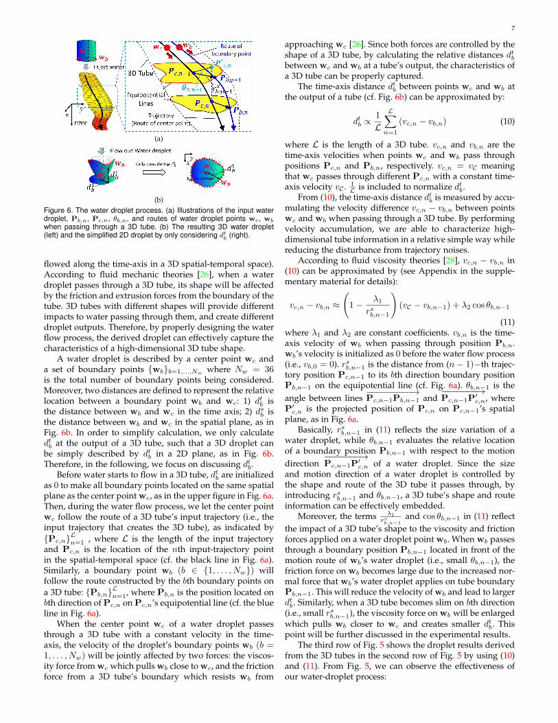
(a)

(b)Figure 6. The water droplet process. (a) Illustrations of the input waterdroplet, Pb,n, Pc,n, θb,n, and routes of water droplet points wc, wb

when passing through a 3D tube. (b) The resulting 3D water droplet(left) and the simplified 2D droplet by only considering dtb (right).

flowed along the time-axis in a 3D spatial-temporal space).According to fluid mechanic theories [26], when a waterdroplet passes through a 3D tube, its shape will be affectedby the friction and extrusion forces from the boundary of thetube. 3D tubes with different shapes will provide differentimpacts to water passing through them, and create differentdroplet outputs. Therefore, by properly designing the waterflow process, the derived droplet can effectively capture thecharacteristics of a high-dimensional 3D tube shape.

A water droplet is described by a center point wc anda set of boundary points {wb}b=1,...,Nw

where Nw = 36is the total number of boundary points being considered.Moreover, two distances are defined to represent the relativelocation between a boundary point wb and wc: 1) dtb isthe distance between wb and wc in the time axis; 2) dsb isthe distance between wb and wc in the spatial plane, as inFig. 6b. In order to simplify calculation, we only calculatedtb at the output of a 3D tube, such that a 3D droplet canbe simply described by dtb in a 2D plane, as in Fig. 6b.Therefore, in the following, we focus on discussing dtb.

Before water starts to flow in a 3D tube, dtb are initializedas 0 to make all boundary points located on the same spatialplane as the center point wc, as in the upper figure in Fig. 6a.Then, during the water flow process, we let the center pointwc follow the route of a 3D tube’s input trajectory (i.e., theinput trajectory that creates the 3D tube), as indicated by{Pc,n}Ln=1 , where L is the length of the input trajectoryand Pc,n is the location of the nth input-trajectory pointin the spatial-temporal space (cf. the black line in Fig. 6a).Similarly, a boundary point wb (b ∈ {1, . . . , Nw}) willfollow the route constructed by the bth boundary points ona 3D tube: {Pb,n}Ln=1, where Pb,n is the position located onbth direction of Pc,n on Pc,n’s equipotential line (cf. the blueline in Fig. 6a).

When the center point wc of a water droplet passesthrough a 3D tube with a constant velocity in the time-axis, the velocity of the droplet’s boundary points wb (b =1, . . . , Nw) will be jointly affected by two forces: the viscos-ity force from wc which pulls wb close to wc, and the frictionforce from a 3D tube’s boundary which resists wb from

approaching wc [26]. Since both forces are controlled by theshape of a 3D tube, by calculating the relative distances dtbbetween wc and wb at a tube’s output, the characteristics ofa 3D tube can be properly captured.

The time-axis distance dtb between points wc and wb atthe output of a tube (cf. Fig. 6b) can be approximated by:

dtb ∝1

L

L∑n=1

(vc,n − vb,n) (10)

where L is the length of a 3D tube. vc,n and vb,n are thetime-axis velocities when points wc and wb pass throughpositions Pc,n and Pb,n, respectively. vc,n = vC meaningthat wc passes through different Pc,n with a constant time-axis velocity vC . 1

L is included to normalize dtb.From (10), the time-axis distance dtb is measured by accu-

mulating the velocity difference vc,n − vb,n between pointswc and wb when passing through a 3D tube. By performingvelocity accumulation, we are able to characterize high-dimensional tube information in a relative simple way whilereducing the disturbance from trajectory noises.

According to fluid viscosity theories [28], vc,n − vb,n in(10) can be approximated by (see Appendix in the supple-mentary material for details):

vc,n − vb,n ≈(

1− λ1

rsb,n−1

)(vC − vb,n−1) + λ2 cos θb,n−1

(11)where λ1 and λ2 are constant coefficients. vb,n is the time-axis velocity of wb when passing through position Pb,n.wb’s velocity is initialized as 0 before the water flow process(i.e., vb,0 = 0). rsb,n−1 is the distance from (n− 1)−th trajec-tory position Pc,n−1 to its bth direction boundary positionPb,n−1 on the equipotential line (cf. Fig. 6a). θb,n−1 is theangle between lines

−−−−−−−−−→Pc,n−1Pb,n−1 and

−−−−−−−→Pc,n−1P

′c,n, where

P′c,n is the projected position of Pc,n on Pc,n−1’s spatialplane, as in Fig. 6a.

Basically, rsb,n−1 in (11) reflects the size variation of awater droplet, while θb,n−1 evaluates the relative locationof a boundary position Pb,n−1 with respect to the motiondirection

−−−−−−−→Pc,n−1P

′c,n of a water droplet. Since the size

and motion direction of a water droplet is controlled bythe shape and route of the 3D tube it passes through, byintroducing rsb,n−1 and θb,n−1, a 3D tube’s shape and routeinformation can be effectively embedded.

Moreover, the terms λ1

rsb,n−1and cos θb,n−1 in (11) reflect

the impact of a 3D tube’s shape to the viscosity and frictionforces applied on a water droplet point wb. When wb passesthrough a boundary position Pb,n−1 located in front of themotion route of wb’s water droplet (i.e., small θb,n−1), thefriction force on wb becomes large due to the increased nor-mal force that wb’s water droplet applies on tube boundaryPb,n−1. This will reduce the velocity of wb and lead to largerdtb. Similarly, when a 3D tube becomes slim on bth direction(i.e., small rsb,n−1), the viscosity force on wb will be enlargedwhich pulls wb closer to wc and creates smaller dtb. Thispoint will be further discussed in the experimental results.

The third row of Fig. 5 shows the droplet results derivedfrom the 3D tubes in the second row of Fig. 5 by using (10)and (11). From Fig. 5, we can observe the effectiveness ofour water-droplet process:

8

• The major motion directions of 3D tubes are properlycaptured by the large sectors in droplet results. Forexample, the water droplet of trajectory C has a largesector in the upward direction since trajectory C movesforward only. Comparatively, the water droplet of trajec-tory B has large sectors in both top and left directions.This indicates the ‘forward+left turn’ movement of B.• Droplets derived from thick 3D tubes have larger sizes

than those derived from slim tubes. For example, thedroplet for trajectory C has large size since C followsa frequent motion pattern in the scene and has a thick3D tube. Comparatively, since trajectory A turns to anirregular region in the middle, its 3D tube becomesnarrow in the later part. This leads to a small size inits corresponding droplet. Fig. 5 implies that the size of adroplet can effectively differentiate regular and irregularmotion patterns. Therefore, in this paper, droplet sizeis utilized as a major feature to detect abnormalities intrajectory analysis (cf. (13)).Finally, the obtained water droplet is sampled to achieve

a low-dimensional droplet vector. In this paper, we simplyconcatenate time-axis distances dtb in a water droplet as thelow-dimensional droplet vector:

Vm = [dt,m1 , dt,m2 , . . . , dt,mNw] (12)

where Vm is the droplet vector for trajectory Γm. dt,mb is thetime-axis distance in bth direction of Γm’s water droplet.Nwis the length of the vector and is set as 36 in our experiments.

5 IMPLEMENTATION IN TRAJECTORY ANALYSIS

With the tube-and-droplet representation, trajectories canbe depicted by droplet vectors and analyzed accordingly.In this section, we discuss the implementations of ourtube-and-droplet representation in three trajectory analysisapplications: trajectory clustering, trajectory classification &abnormality detection, and 3D action recognition.

5.1 Trajectory Clustering

When performing trajectory clustering, we first utilize alltrajectories being clustered as the given trajectories to con-struct thermal transfer fields (cf. Section 3.1). Then, a 3Dtube and a droplet vector are derived based on the con-structed thermal transfer fields to represent each trajectory(cf. Sections 3.3 and 4). Finally, we measure the distancebetween trajectories by calculating the distance betweentheir corresponding droplet vectors, and perform trajectoryclustering according to these droplet-vector distances. Inthis paper, we utilize Euclidean distance to measure the dis-tance between droplet vectors, and utilize spectral clustering[29] to cluster trajectories.

5.2 Trajectory Classification & Abnormality Detection

In trajectory classification and abnormality detection, a set ofnormal training trajectories are provided whose class labelsare given. We aim to recognize the classes of input testtrajectories with the guidance of training trajectories, andidentify abnormal test trajectories which do not follow theregular motion patterns provided by training trajectories.

Figure 7. An example of 3D skeleton sequence from MSR-Action3Ddataset. Left: The 3D trajectory of ‘horizontal wave’ action of a ‘left hand’body point. Right: The skeleton sequence for ‘horizontal wave’ action.

Similar to trajectory clustering, we utilize all normaltrajectories in the training set to construct thermal trans-fer fields, and derive a droplet vector for each individualtraining trajectory. Note that since our approach utilizesthe complete contextual information, we do not differentiatetrajectory classes, that is, normal training trajectories fromdifferent trajectory classes are utilized indiscriminativelywhen constructing thermal transfer fields.

During testing, we first obtain a droplet vector for aninput test trajectory. Then, the abnormality of a test trajec-tory is evaluated by its corresponding droplet vector. Sincethe size of a droplet can effectively differentiate regular andirregular motion patterns, we detect a test trajectory Γm tobe abnormal if:

maxb{dt,mb }+

1

Nw

∑b

dt,mb < TH (13)

where dt,mb is the bth element in Γm’s droplet vector. Nw isthe length of the droplet vector (cf. (12)). TH is a thresholddecided by specific scenario. In the experiments of thispaper, we simply calculate maxb {dt,mb }+ 1

Nw

∑b d

t,mb value

for all normal trajectories in the training set, select thesmallest value T from them, and set 0.9T as the threshold. In(13), the term 1

Nw

∑b d

t,mb is calculated to measure the size

of a droplet while the term maxb {dt,mb } is used to evaluatethe normality in a trajectory’s major motion direction.

Finally, if a test trajectory Γm is evaluated as normalby (13), a one-against-all linear SVM classifier [30] traineddirectly from the droplet vectors of training trajectories isapplied to classify Γm into one of the trajectory classes.

5.3 3D Action Recognition

We also extend our tube-and-droplet approach into the ap-plication of 3D action recognition. In 3D action recognition,3D skeleton sequences are provided which depict humanactions in a 3D x-y-depth space [31]–[35]. An exampleskeleton sequence is shown in Fig. 7.

Since skeleton sequences are described by the trajectoriesof multiple body points (e.g., the red curve in Fig. 7),they are able to be represented and analyzed by the pro-posed tube-and-droplet approach. However, a 3D skeletonsequence differs from a regular motion trajectory in: 1) A 3Dskeleton sequence includes multiple trajectories for differentbody points of a human; 2) The trajectory of a body pointis located in 3D space (x-y-depth) instead of a 2D plane.Therefore, we extend our tube-and-droplet representationinto higher dimension to depict 3D trajectories. Besides,in order to handle multiple trajectories in a 3D skeletonsequence, we represent each trajectory independently and

9

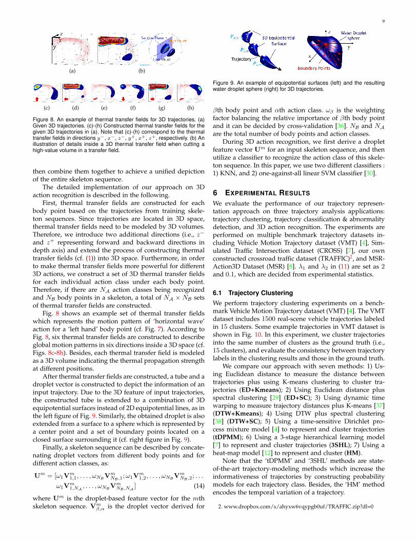
(a) (b)

(c) (d) (e) (f) (g) (h)

Figure 8. An example of thermal transfer fields for 3D trajectories. (a)Given 3D trajectories. (c)-(h) Constructed thermal transfer fields for thegiven 3D trajectories in (a). Note that (c)-(h) correspond to the thermaltransfer fields in directions y−, x−, z−, y+, x+, z+, respectively. (b) Anillustration of details inside a 3D thermal transfer field when cutting ahigh-value volume in a transfer field.

then combine them together to achieve a unified depictionof the entire skeleton sequence.

The detailed implementation of our approach on 3Daction recognition is described in the following.

First, thermal transfer fields are constructed for eachbody point based on the trajectories from training skele-ton sequences. Since trajectories are located in 3D space,thermal transfer fields need to be modeled by 3D volumes.Therefore, we introduce two additional directions (i.e., z−

and z+ representing forward and backward directions indepth axis) and extend the process of constructing thermaltransfer fields (cf. (1)) into 3D space. Furthermore, in orderto make thermal transfer fields more powerful for different3D actions, we construct a set of 3D thermal transfer fieldsfor each individual action class under each body point.Therefore, if there are NA action classes being recognizedand NB body points in a skeleton, a total of NA × NB setsof thermal transfer fields are constructed.

Fig. 8 shows an example set of thermal transfer fieldswhich represents the motion pattern of ‘horizontal wave’action for a ‘left hand’ body point (cf. Fig. 7). According toFig. 8, six thermal transfer fields are constructed to describeglobal motion patterns in six directions inside a 3D space (cf.Figs. 8c-8h). Besides, each thermal transfer field is modeledas a 3D volume indicating the thermal propagation strengthat different positions.

After thermal transfer fields are constructed, a tube and adroplet vector is constructed to depict the information of aninput trajectory. Due to the 3D feature of input trajectories,the constructed tube is extended to a combination of 3Dequipotential surfaces instead of 2D equipotential lines, as inthe left figure of Fig. 9. Similarly, the obtained droplet is alsoextended from a surface to a sphere which is represented bya center point and a set of boundary points located on aclosed surface surrounding it (cf. right figure in Fig. 9).

Finally, a skeleton sequence can be described by concate-nating droplet vectors from different body points and fordifferent action classes, as:

Um = [ω1Vm1,1, . . . , ωNBV

mNB,1;ω1V

m1,2, . . . , ωNBV

mNB,2; . . .

ω1Vm1,NA , . . . , ωNBV

mNB,NA ] (14)

where Um is the droplet-based feature vector for the mthskeleton sequence. Vm

β,α is the droplet vector derived for

Figure 9. An example of equipotential surfaces (left) and the resultingwater droplet sphere (right) for 3D trajectories.

βth body point and αth action class. ωβ is the weightingfactor balancing the relative importance of βth body pointand it can be decided by cross-validation [36]. NB and NAare the total number of body points and action classes.

During 3D action recognition, we first derive a dropletfeature vector Um for an input skeleton sequence, and thenutilize a classifier to recognize the action class of this skele-ton sequence. In this paper, we use two different classifiers :1) KNN, and 2) one-against-all linear SVM classifier [30].

6 EXPERIMENTAL RESULTS

We evaluate the performance of our trajectory represen-tation approach on three trajectory analysis applications:trajectory clustering, trajectory classification & abnormalitydetection, and 3D action recognition. The experiments areperformed on multiple benchmark trajectory datasets in-cluding Vehicle Motion Trajectory dataset (VMT) [4], Sim-ulated Traffic Intersection dataset (CROSS) [7], our ownconstructed crossroad traffic dataset (TRAFFIC)2, and MSR-Action3D Dataset (MSR) [8]. λ1 and λ2 in (11) are set as 2and 0.1, which are decided from experimental statistics.

6.1 Trajectory ClusteringWe perform trajectory clustering experiments on a bench-mark Vehicle Motion Trajectory dataset (VMT) [4]. The VMTdataset includes 1500 real-scene vehicle trajectories labeledin 15 clusters. Some example trajectories in VMT dataset isshown in Fig. 10. In this experiment, we cluster trajectoriesinto the same number of clusters as the ground truth (i.e.,15 clusters), and evaluate the consistency between trajectorylabels in the clustering results and those in the ground truth.

We compare our approach with seven methods: 1) Us-ing Euclidean distance to measure the distance betweentrajectories plus using K-means clustering to cluster tra-jectories (ED+Kmeans); 2) Using Euclidean distance plusspectral clustering [29] (ED+SC); 3) Using dynamic timewarping to measure trajectory distances plus K-means [37](DTW+Kmeans); 4) Using DTW plus spectral clustering[38] (DTW+SC); 5) Using a time-sensitive Dirichlet pro-cess mixture model [4] to represent and cluster trajectories(tDPMM); 6) Using a 3-stage hierarchical learning model[7] to represent and cluster trajectories (3SHL); 7) Using aheat-map model [12] to represent and cluster (HM).

Note that the ‘tDPMM’ and ‘3SHL’ methods are state-of-the-art trajectory-modeling methods which increase theinformativeness of trajectories by constructing probabilitymodels for each trajectory class. Besides, the ‘HM’ methodencodes the temporal variation of a trajectory.

2. www.dropbox.com/s/ahyxw6vqypgb0uf/TRAFFIC.zip?dl=0

10

Table 1Cluster Learning Accuracy for different methods on VMT Dataset (%)

Method Cluster AccuracyED+Kmeans 82.6ED+SC [29] 85.0DTW+Kmeans [37] 83.2DTW+SC [38] 85.3tDPMM [4] 86.73SHL [7] 84.4HM [12] 82.03D Tube+Hausdorff 91.5Thermal Map+Manifold 92.23D Tube+Manifold 93.6Ours 93.8

Moreover, in order to evaluate the effectiveness of ourwater droplet process, we further include the results ofthree additional methods: 1) Using our approach to con-struct 3D tubes for trajectory representation, plus usingHausdorff distance [24] to capture the high-dimensionalinformation in these 3D tubes for trajectory clustering(3D Tube+Hausdorff); 2) Using 3D tubes plus usinga state-of-the-art Grassmann manifold method [20] (3DTube+Manifold); 3) Using our approach to achieve thermaldiffusion maps for each trajectory point (cf. Fig. 3), anddirectly concatenating these thermal diffusion maps as therepresentation of a trajectory, finally using the Grassmannmanifold method [20] to capture the high-dimensional in-formation (Thermal map+Manifold).

Note that the major difference between the ‘Thermalmap+Manifold’ method and ‘3D Tube+Manifold’ methodis that ‘Thermal map+Manifold’ skips the step of equipo-tential line extraction (cf. Section 3.2), and directly utilizes athermal diffusion map to represent a trajectory point.

6.1.1 Comparison of clustering results

Table 1 compares the cluster learning accuracy [4] for dif-ferent methods on VMT dataset, where the cluster learn-ing accuracy measures the total percentage of trajectoriesbeing correctly clustered. From Table 1, approaches us-ing our 3D tube representation (3D Tube+Hausdorff, 3DTube+Manifold, Thermal map+Manifold, Ours) achieve ob-viously better clustering results than the compared meth-ods. This demonstrates the usefulness of our 3D tube rep-resentation. Moreover, we can also observe from Table 1that: 1) Our approach, which integrates both 3D tube rep-resentation and water droplet process, achieves the bestclustering results. This demonstrates the effectiveness ofour tube+droplet framework. 2) The ‘3D Tube+Manifold’method has slightly better results than the ‘Thermalmap+Manifold’ method. This implies that equipotentiallines (cf. Section 3.2) can not only capture the useful infor-mation in thermal diffusion maps, but also suitably avoidthe disturbance from noise in thermal diffusion maps.

6.1.2 Robustness to noises and trajectory breaks

We further demonstrate the effectiveness of our approach indealing with noisy or broken trajectories. Following [4], weadd Gaussian noise to all points in a trajectory to simulate anoisy trajectory. Three noise levels are used to derive threetrajectory datasets with different noise strengths (i.e., Noise

Level 1, 2, and 3 in Table 2). Similarly, we omit the initialor last G points in two of 10 trajectories in each cluster tosimulate datasets with broken trajectories (i.e., omit G =10%, G = 20%, G = 30%, and G = 40% in Table 2) [4].

Table 2 compares the clustering results of different meth-ods on noisy or broken trajectories derived from VMTdataset. Table 2 shows that our approach achieves thebest clustering results under different noise or trajectorybreak levels. Moreover, when noise or trajectory break levelincreases, the clustering performance decrease by our ap-proach is relatively small among the compared methods,this further demonstrates the robustness of our tube-and-droplet approach when handling noises or trajectory breaks.

6.1.3 Effectiveness of 3D tube representation

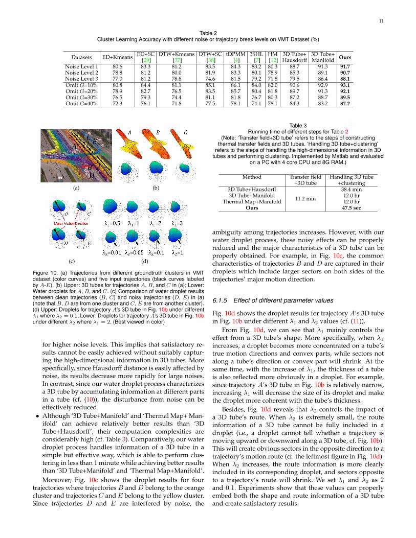
Figs 10 illustrates a more detailed example about the ef-fectiveness of our 3D tube representation. In Fig. 10a, thecolored curves are trajectories to be clustered and the blacktrajectories labeled in A, B, and C are three trajectoriesfrom them. In order to ease the discussion, trajectories fromdifferent groundtruth clusters are displayed by differentcolors. Since trajectories A, B, and C come from threetrajectory clusters which are located close to each otherand have similar motion patterns (cf. the clusters in yellow,orange, and red in Fig. 10a), existing methods have limita-tions in differentiating them which only consider the pair-wise correlation between trajectories (ED+Kmeans, ED+SC,DTW+Kmeans, DTW+SC, HM) or intra-cluster correlationamong trajectories (tDPMM, 3SHL).

With our 3D tube representation, the differences amongA, B, and C can be properly highlighted by embeddingthe complete motion information from all trajectories, asthe upper figures in Fig. 10b. For example, the 3D tube oftrajectory A shows an obvious leftward convex part sincethere is a large left-turn pattern provided by the purplecluster along A’s route. Trajectory B’s tube is thicker sinceit is located in the middle of a large upleft-ward motionpattern jointly provided by the yellow, orange, and redclusters. Besides, trajectory C’s tube includes an obviousrightward convex part due to the rightward contextualpatterns provided by the blue and green clusters next to C .Therefore, by suitably capturing the high-dimensional infor-mation in these 3D tubes, the difference among trajectoriescan be effectively reflected in the resulting droplet vectors(cf. the lower figures in Fig. 10b).

6.1.4 Effectiveness of water droplet process

In order to evaluate our water droplet process, wecompare our approach with ‘3D Tube+Hausdorff’, ‘3DTube+Manifold’, and ‘Thermal Map+Manifold’. Thesemethods use the same 3D tube representation to depict atrajectory, but use different schemes to capture the high-dimensional information in a 3D tube. The clustering resultsof these methods under different noise or trajectory breaklevels are shown in Table 2. Furthermore, Table 3 comparesthe running time of the 3D tube information handling &clustering steps in these methods. We observe that:• From Table 2, the clustering-accuracy difference between

our approach and ‘3D Tube+Hausdorff’ becomes larger

11

Table 2Cluster Learning Accuracy with different noise or trajectory break levels on VMT Dataset (%)

Datasets ED+Kmeans ED+SC[29]

DTW+Kmeans[37]

DTW+SC[38]

tDPMM[4]

3SHL[7]

HM[12]

3D Tube+Hausdorff

3D Tube+Manifold Ours

Noise Level 1 80.6 83.3 81.2 83.5 84.3 83.2 80.3 88.7 91.3 91.7Noise Level 2 78.8 81.2 80.0 81.9 83.3 80.1 78.9 85.3 89.1 90.7Noise Level 3 77.0 81.2 78.8 74.6 81.5 79.2 71.8 79.5 86.4 88.1Omit G=10% 80.8 84.4 81.1 85.1 86.1 84.0 82.0 90.6 92.9 93.1Omit G=20% 78.9 82.7 76.5 83.5 85.7 80.4 81.8 89.7 91.3 92.1Omit G=30% 76.5 79.3 74.4 81.1 81.8 76.7 80.3 87.2 88.7 89.5Omit G=40% 72.3 76.1 71.8 77.5 78.1 74.1 78.1 84.3 83.2 87.2

(a) (b)

(c) (d)

Figure 10. (a) Trajectories from different groundtruth clusters in VMTdataset (color curves) and five input trajectories (black curves labeledby A-E). (b) Upper: 3D tubes for trajectories A, B, and C in (a); Lower:Water droplets for A, B, and C. (c) Comparison of water droplet resultsbetween clean trajectories (B, C) and noisy trajectories (D, E) in (a)(note that B, D are from one cluster and C, E are from another cluster).(d) Upper: Droplets for trajectory A’s 3D tube in Fig. 10b under differentλ1 where λ2 = 0.1; Lower: Droplets for trajectoryA’s 3D tube in Fig. 10bunder different λ2 where λ1 = 2. (Best viewed in color)

for higher noise levels. This implies that satisfactory re-sults cannot be easily achieved without suitably captur-ing the high-dimensional information in 3D tubes. Morespecifically, since Hausdorff distance is easily affected bynoise, its results decrease more rapidly for large noises.In contrast, since our water droplet process characterizesa 3D tube by accumulating information at different partsin a tube (cf. (10)), the disturbance from noise can beeffectively reduced.• Although ‘3D Tube+Manifold’ and ‘Thermal Map+ Man-

ifold’ can achieve relatively better results than ‘3DTube+Hausdorff’, their computation complexities areconsiderably high (cf. Table 3). Comparatively, our waterdroplet process handles information of a 3D tube in asimple but effective way, which is able to perform clus-tering in less than 1 minute while achieving better resultsthan ‘3D Tube+Manifold’ and ‘Thermal Map+Manifold’.Moreover, Fig. 10c shows the droplet results for four

trajectories where trajectories B and D belong to the orangecluster and trajectories C andE belong to the yellow cluster.Since trajectories D and E are interfered by noise, the

Table 3Running time of different steps for Table 2

(Note: ‘Transfer field+3D tube’ refers to the steps of constructingthermal transfer fields and 3D tubes. ‘Handling 3D tube+clustering’

refers to the steps of handling the high-dimensional information in 3Dtubes and performing clustering. Implemented by Matlab and evaluated

on a PC with 4 core CPU and 8G RAM.)

Method Transfer field Handling 3D tube+3D tube +clustering

3D Tube+Hausdorff

11.2 min

38.4 min3D Tube+Manifold 12.0 hr

Thermal Map+Manifold 12.0 hrOurs 47.5 sec

ambiguity among trajectories increases. However, with ourwater droplet process, these noisy effects can be properlyreduced and the major characteristics of a 3D tube can beproperly obtained. For example, in Fig. 10c, the commoncharacteristics of trajectories B and D are captured in theirdroplets which include larger sectors on both sides of thetrajectories’ major motion direction.

6.1.5 Effect of different parameter values

Fig. 10d shows the droplet results for trajectory A’s 3D tubein Fig. 10b under different λ1 and λ2 values (cf. (11)).

From Fig. 10d, we can see that λ1 mainly controls theeffect from a 3D tube’s shape. More specifically, when λ1

increases, a droplet becomes more concentrated on a tube’strue motion directions and convex parts, while sectors notalong a tube’s direction or convex part will shrink. At thesame time, with the increase of λ1, the thickness of a tubeis also reflected more obviously in a droplet. For example,since trajectory A’s 3D tube in Fig. 10b is relatively narrow,increasing λ1 will decrease the size of its droplet and makethe droplet more coherent with the tube’s thickness.

Besides, Fig. 10d reveals that λ2 controls the impact ofa 3D tube’s route. When λ2 is extremely small, the routeinformation of a 3D tube cannot be fully included in adroplet (i.e., a droplet cannot tell whether a trajectory ismoving upward or downward along a 3D tube, cf. Fig. 10b).This will create obvious sectors in the opposite direction to atrajectory’s motion route (cf. the leftmost figure in Fig. 10d).When λ2 increases, the route information is more clearlyincluded in its corresponding droplet, and sectors oppositeto a trajectory’s route will shrink. We set λ1 and λ2 as 2and 0.1. Experiments show that these values can properlyembed both the shape and route information of a 3D tubeand create satisfactory results.

12

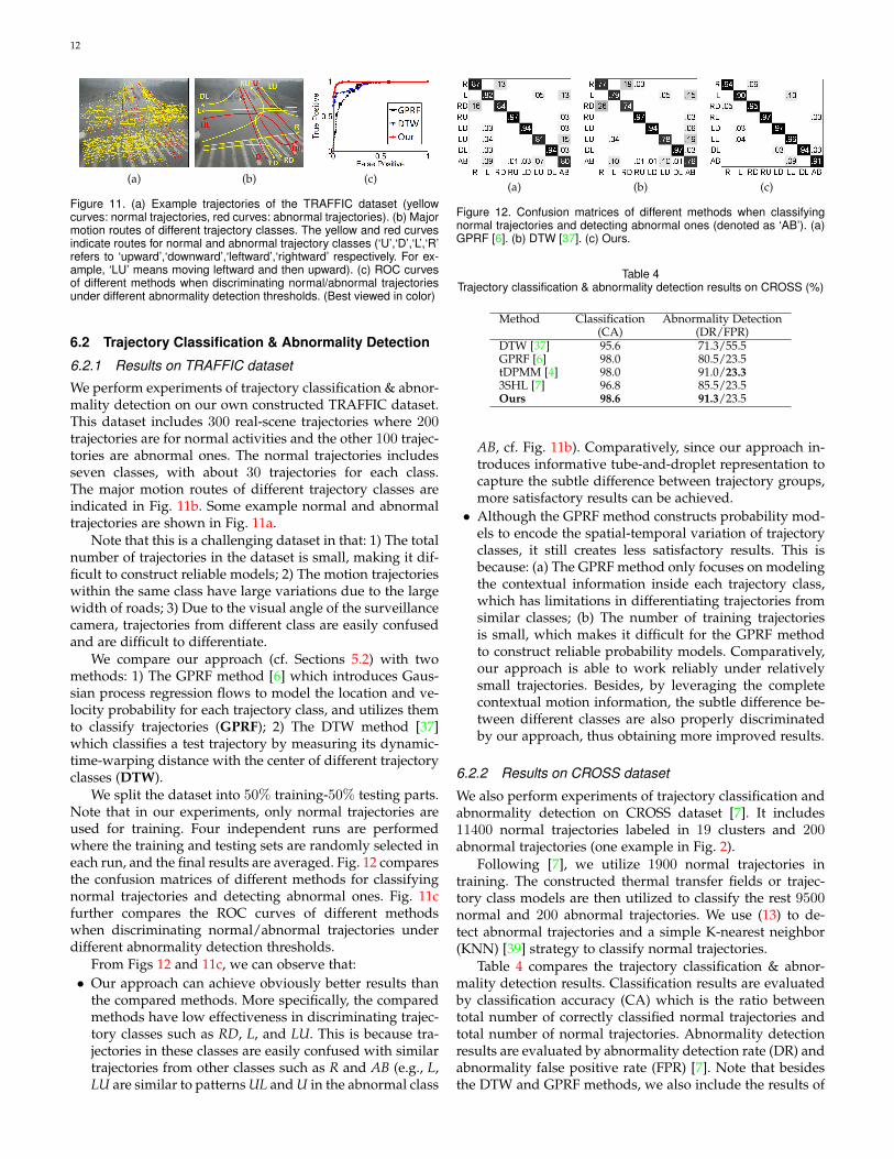
(a) (b) (c)

Figure 11. (a) Example trajectories of the TRAFFIC dataset (yellowcurves: normal trajectories, red curves: abnormal trajectories). (b) Majormotion routes of different trajectory classes. The yellow and red curvesindicate routes for normal and abnormal trajectory classes (‘U’,‘D’,‘L’,‘R’refers to ‘upward’,‘downward’,‘leftward’,‘rightward’ respectively. For ex-ample, ‘LU’ means moving leftward and then upward). (c) ROC curvesof different methods when discriminating normal/abnormal trajectoriesunder different abnormality detection thresholds. (Best viewed in color)

6.2 Trajectory Classification & Abnormality Detection

6.2.1 Results on TRAFFIC dataset

We perform experiments of trajectory classification & abnor-mality detection on our own constructed TRAFFIC dataset.This dataset includes 300 real-scene trajectories where 200trajectories are for normal activities and the other 100 trajec-tories are abnormal ones. The normal trajectories includesseven classes, with about 30 trajectories for each class.The major motion routes of different trajectory classes areindicated in Fig. 11b. Some example normal and abnormaltrajectories are shown in Fig. 11a.

Note that this is a challenging dataset in that: 1) The totalnumber of trajectories in the dataset is small, making it dif-ficult to construct reliable models; 2) The motion trajectorieswithin the same class have large variations due to the largewidth of roads; 3) Due to the visual angle of the surveillancecamera, trajectories from different class are easily confusedand are difficult to differentiate.

We compare our approach (cf. Sections 5.2) with twomethods: 1) The GPRF method [6] which introduces Gaus-sian process regression flows to model the location and ve-locity probability for each trajectory class, and utilizes themto classify trajectories (GPRF); 2) The DTW method [37]which classifies a test trajectory by measuring its dynamic-time-warping distance with the center of different trajectoryclasses (DTW).

We split the dataset into 50% training-50% testing parts.Note that in our experiments, only normal trajectories areused for training. Four independent runs are performedwhere the training and testing sets are randomly selected ineach run, and the final results are averaged. Fig. 12 comparesthe confusion matrices of different methods for classifyingnormal trajectories and detecting abnormal ones. Fig. 11cfurther compares the ROC curves of different methodswhen discriminating normal/abnormal trajectories underdifferent abnormality detection thresholds.

From Figs 12 and 11c, we can observe that:• Our approach can achieve obviously better results than

the compared methods. More specifically, the comparedmethods have low effectiveness in discriminating trajec-tory classes such as RD, L, and LU. This is because tra-jectories in these classes are easily confused with similartrajectories from other classes such as R and AB (e.g., L,LU are similar to patterns UL and U in the abnormal class

(a) (b) (c)

Figure 12. Confusion matrices of different methods when classifyingnormal trajectories and detecting abnormal ones (denoted as ‘AB’). (a)GPRF [6]. (b) DTW [37]. (c) Ours.

Table 4Trajectory classification & abnormality detection results on CROSS (%)

Method Classification Abnormality Detection(CA) (DR/FPR)

DTW [37] 95.6 71.3/55.5GPRF [6] 98.0 80.5/23.5tDPMM [4] 98.0 91.0/23.33SHL [7] 96.8 85.5/23.5Ours 98.6 91.3/23.5

AB, cf. Fig. 11b). Comparatively, since our approach in-troduces informative tube-and-droplet representation tocapture the subtle difference between trajectory groups,more satisfactory results can be achieved.• Although the GPRF method constructs probability mod-

els to encode the spatial-temporal variation of trajectoryclasses, it still creates less satisfactory results. This isbecause: (a) The GPRF method only focuses on modelingthe contextual information inside each trajectory class,which has limitations in differentiating trajectories fromsimilar classes; (b) The number of training trajectoriesis small, which makes it difficult for the GPRF methodto construct reliable probability models. Comparatively,our approach is able to work reliably under relativelysmall trajectories. Besides, by leveraging the completecontextual motion information, the subtle difference be-tween different classes are also properly discriminatedby our approach, thus obtaining more improved results.

6.2.2 Results on CROSS dataset

We also perform experiments of trajectory classification andabnormality detection on CROSS dataset [7]. It includes11400 normal trajectories labeled in 19 clusters and 200abnormal trajectories (one example in Fig. 2).

Following [7], we utilize 1900 normal trajectories intraining. The constructed thermal transfer fields or trajec-tory class models are then utilized to classify the rest 9500normal and 200 abnormal trajectories. We use (13) to de-tect abnormal trajectories and a simple K-nearest neighbor(KNN) [39] strategy to classify normal trajectories.

Table 4 compares the trajectory classification & abnor-mality detection results. Classification results are evaluatedby classification accuracy (CA) which is the ratio betweentotal number of correctly classified normal trajectories andtotal number of normal trajectories. Abnormality detectionresults are evaluated by abnormality detection rate (DR) andabnormality false positive rate (FPR) [7]. Note that besidesthe DTW and GPRF methods, we also include the results of

13

two state-of-the-art methods on CROSS dataset in Table 4(i.e., 3SHL [7] and tDPMM [4]).

Our approach achieves the best performance in classifi-cation. When detecting abnormal trajectories, our approachcan also achieve obviously improved results than the com-pared methods (DTW [37], 3SHL [7], and GPRF [6]) andsimilar results to a state-of-the-art tDPMM method [4].

6.3 3D Action Recognition

Finally, we evaluate the performance of our approach in 3Daction recognition. We perform experiments on a benchmarkMSR-Action3D Dataset [8] which includes 557 3D skeletonsequences for 20 human actions performed by 10 differentsubjects. One example skeleton sequence is shown in Fig. 7.

Following the previous works on MSR-Action3D dataset[8], [40], we evaluate the recognition accuracy over all 20actions where actions of half of the subjects are used fortraining and the rest actions are used for testing. Besides, atrajectory alignment process similar to [31] is applied as apre-processing step to reduce 3D trajectory variations.

We utilize the process in Section 5.3 to implement ourapproach for 3D action recognition, where ‘Droplet+KNN’and ‘Droplet+SVM’ in Table 5 refer to using KNN andSVM classifiers to recognize our droplet feature vectors (cf.(14)), respectively. Moreover, we also include the results bycombining our droplet feature vector with a state-of-the-art‘Moving Poselets’ method [41] which introduces sophisti-cated mid-level classifiers to improve recognition accuracy(cf. ‘Droplet+Moving Poselets’ in Table 5). Specifically, weconcatenate our droplet feature vectors with the body pointvelocity & acceleration features used in [41], and follow the‘Moving Poselets’ classification process [41] to recognize theaction class of the concatenated feature vectors.

We compare our approach with the state-of-the-art 3Daction recognition methods using skeleton sequences [32]–[35], [40]–[43]. Table 5 shows the recognition accuracy. Ac-cording to Table 5, our ‘Droplet+SVM’ approach outper-forms all the existing techniques except [41]. This demon-strates that our tube-and-droplet framework can be reliablyapplied to handle sequence analysis with multiple trajec-tories. Besides, our ‘Droplet+KNN’ approach also achievessatisfactory results. It implies that our droplet featurescan effectively capture the discriminative characteristics oftrajectories, such that good results can be achieved withsimple recognition strategies such as KNN. Moreover, the‘Droplet+Moving Poselets’ approach achieves the best per-formance. It further indicates that our droplet features canbe effectively combined with more sophisticated recognitionstrategies to achieve further improved performances.

7 CONCLUSION

In this paper, we study the problem of informative trajec-tory representation and introduce a novel tube-and-dropletframework. The framework consists of three key ingredi-ents: 1) introducing the idea of constructing thermal transferfields to embed the global motion patterns in a scene; 2)deriving equipotential lines and concatenating them into a3D tube to establish a highly informative representation,which properly embeds both the motion route and the

Table 5Recognition accuracy comparison on MSR-Action3D dataset (%)

Method Recognition AccuracyEigen joints [42] 82.3HON4D+Ddisc [40] 88.9Actionlet Ensemble [32] 88.2Skeleton Quads [34] 89.9Pose Set [43] 90.2Manifold Learning [35] 91.2Moving Pose [33] 91.7Moving Poselets [41] 93.6Droplet+KNN 91.2Droplet+SVM 92.1Droplet+Moving Poselets 93.9

contextual motion pattern for a trajectory; 3) introducinga simple but effective droplet-based process to effectivelycapture the rich information in 3D tube representation. Weapply our tube-and-droplet approach to various trajectoryanalysis applications including clustering, abnormality de-tection, and 3D action recognition. Extensive experiments onbenchmark demonstrate the effectiveness of our approach.

REFERENCES

[1] X. Wang, K. Tieu, and E. Grimson, “Learning semantic scene mod-els by trajectory analysis,” in Proc. European Conf. Comp. Vision,2006, pp. 110–123.

[2] J. J. Little and Z. Gu, “Video retrieval by spatial and temporalstructure of trajectories,” in Proc. of SPIE, 2001, pp. 545–552.

[3] Y.-K. Jung, K.-W. Lee, and Y.-S. Ho, “Content-based event retrievalusing semantic scene interpretation for automated traffic surveil-lance,” IEEE Trans. Intell. Transp. Syst., vol. 2, pp. 151–163, 2001.

[4] W. Hu, X. Li, G. Tian, S. Maybank, and Z. Zhang, “An incremen-tal dpmm-based method for trajectory clustering, modeling, andretrieval,” IEEE Trans. Pattern Anal. Mach. Intell., vol. 35, no. 5, pp.1051–1065, 2013.

[5] H. Xu, Y. Zhou, W. Lin, and H. Zha, “Unsupervised trajectoryclustering via adaptive multi-kernel-based shrinkage,” in Proc.IEEE Intl. Conf. Comp. Vision, 2015, pp. 4328–4336.

[6] K. Kim, D. Lee, and I. Essa, “Gaussian process regression flowfor analysis of motion trajectories,” in Proc. IEEE Intl. Conf. Comp.Vision, 2011, pp. 1164–1171.

[7] B. T. Morris and M. M. Trivedi, “Trajectory learning for activityunderstanding: Unsupervised, multilevel, and long-term adaptiveapproach,” IEEE Trans. Pattern Anal. Mach. Intell., vol. 33, no. 11,pp. 2287–2301, 2011.

[8] W. Li, Z. Zhang, and Z. Liu, “Action recognition based on a bagof 3d points,” in Proc. IEEE Conf. Comp. Vision and Patt. Recog.Workshops, 2010, pp. 9–14.

[9] W. Hu, D. Xie, T. Tan, and S. Maybank, “Learning activity patternsusing fuzzy self-organizing neural network,” IEEE Trans. Syst.,Man, and Cybern. B, vol. 34, no. 3, pp. 1618–1626, 2004.

[10] A. Naftel and S. Khalid, “Motion trajectory learning in the dft-coefficient feature space,” in Proc. IEEE Intl. Conf. Comp. VisionSyst., 2006, pp. 47–47.

[11] T. Palpanas, M. Vlachos, E. Keogh, D. Gunopulos, and W. Truppel,“Online amnesic approximation of streaming time series,” in Proc.Intl. Conf. Data Eng., 2004, pp. 339–349.

[12] W. Lin, H. Chu, J. Wu, B. Sheng, and Z. Chen, “A heat-map-basedalgorithm for recognizing group activities in videos,” IEEE Trans.Circuits Syst. Video Technol., vol. 23, no. 11, pp. 1980–1992, 2015.

[13] X. Wang, K. T. Ma, G.-W. Ng, and W. E. L. Grimson, “Trajectoryanalysis and semantic region modeling using nonparametric hier-archical bayesian models,” Intl. J. Comp. Vision, vol. 95, no. 3, pp.287–312, 2011.

[14] C. Rao, A. Yilmaz, and M. Shah, “View-invariant representationand recognition of actions,” Intl. J. Comp. Vision, vol. 50, no. 2, pp.203–226, 2002.

[15] J. C. Nascimento, M. A. Figueiredo, and J. S. Marques, “Trajectoryclassification using switched dynamical hidden markov models,”IEEE Trans. Image Process., vol. 19, no. 5, pp. 1338–1348, 2010.

14

[16] M. Muller, “Dynamic time warping,” Information Retrieval for Mu-sic and Motion, pp. 69–84, 2007.

[17] M. Vlachos, D. Gunopoulos, and G. Kollios, “Discovering similarmultidimensional trajectories,” in Proc. Intl. Conf. Data Eng., 2002,pp. 673–684.

[18] S. Wold, K. Esbensen, and P. Geladi, “Principal component analy-sis,” Chemometr. Intell. Lab. Syst., vol. 2, no. 1, pp. 37–52, 1987.

[19] G. Baudat and F. Anouar, “Generalized discriminant analysisusing a kernel approach,” Neural Computation, vol. 12, no. 10, pp.2385–2404, 2000.

[20] Y. M. Lui, “Tangent bundles on special manifolds for actionrecognition,” IEEE Trans. Circuits Syst. Video Technol., vol. 22, no. 6,pp. 930–942, 2012.

[21] D. Gong, X. Zhao, and G. Medioni, “Robust multiple manifoldsstructure learning,” in Proc. Intl. Conf. Mach. Learn., 2012, pp. 321–328.

[22] A. Goh and R. Vidal, “Segmenting motions of different types byunsupervised manifold clustering,” in Proc. IEEE Comp. Vision andPatt. Recog., 2007, pp. 1–6.

[23] E. Sangineto, “Pose and expression independent facial landmarklocalization using dense-surf and the hausdorff distance,” IEEETrans. Pattern Anal. Mach. Intell., vol. 35, no. 3, pp. 624–638, 2013.

[24] Y. Gao, M. Wang, R. Ji, X. Wu, and Q. Dai, “3-d object retrieval withhausdorff distance learning,” IEEE Trans. Industrial Electronics,vol. 61, no. 4, pp. 2088–2098, 2014.

[25] S. Patankar, Numerical Heat Transfer and Fluid Flow. CRC Press,1980.

[26] R. H. Pletcher, J. C. Tannehill, and D. Anderson, Computational fluidmechanics and heat transfer. CRC Press, 2012.

[27] J. N. Reddy, An Introduction to Nonlinear Finite Element Analysis:with Applications to Heat Transfer, Fluid Mechanics, and Solid Me-chanics. Oxford University Press, 2014.

[28] B. R. Munson, D. F. Young, and T. H. Okiishi, Fundamentals of FluidMechanics. New York, 1990.

[29] U. Von Luxburg, “A tutorial on spectral clustering,” Statistics andComputing, vol. 17, no. 4, pp. 395–416, 2007.

[30] C.-C. Chang and C.-J. Lin, “LIBSVM: A library for support vectormachines,” ACM Trans. Intell. Syst. Tech., vol. 2, pp. 1–27, 2011.

[31] R. Vemulapalli, F. Arrate, and R. Chellappa, “Human action recog-nition by representing 3d skeletons as points in a lie group,” inProc. IEEE Conf. Comp. Vision and Patt. Recog., 2014, pp. 588–595.

[32] J. Wang, Z. Liu, Y. Wu, and J. Yuan, “Learning actionlet ensemblefor 3d human action recognition,” IEEE Trans. Pattern Anal. Mach.Intell., vol. 36, no. 5, pp. 914–927, 2014.

[33] M. Zanfir, M. Leordeanu, and C. Sminchisescu, “The movingpose: An efficient 3d kinematics descriptor for low-latency actionrecognition and detection,” in Proc. IEEE Intl. Conf. Comp. Vision,2013, pp. 2752–2759.

[34] G. D. Evangelidis, G. Singh, and R. Horaud, “Continuous gesturerecognition from articulated poses,” in Proc. European Conf. Comp.Vision Workshops, 2014, pp. 595–607.

[35] R. Slama, H. Wannous, M. Daoudi, and A. Srivastava, “Accurate3d action recognition using learning on the grassmann manifold,”Pattern Recognition, vol. 48, no. 2, pp. 556–567, 2015.

[36] M. W. Browne, “Cross-validation methods,” Journal of MathematicalPsychology, vol. 44, no. 1, pp. 108–132, 2000.

[37] D. J. Berndt and J. Clifford, “Using dynamic time warping to findpatterns in time series.” in Proc. KDD workshop, vol. 10, no. 16,1994, pp. 359–370.

[38] B. Morris and M. Trivedi, “Learning trajectory patterns by cluster-ing: Experimental studies and comparative evaluation,” in Proc.IEEE Conf. Comp. Vision and Patt. Recog., 2009, pp. 312–319.

[39] K. Fukunaga and L. Hostetler, “K-nearest-neighbor Bayes-riskestimation,” IEEE Trans. Info. Theo., vol. 21, pp. 285 – 293, 1975.

[40] O. Oreifej and Z. Liu, “Hon4d: Histogram of oriented 4d normalsfor activity recognition from depth sequences,” in Proc. IEEE Comp.Vision and Patt. Recog., 2013, pp. 716–723.

[41] L. Tao and R. Vidal, “Moving poselets: A discriminative and inter-pretable skeletal motion representation for action recognition,” inProc. IEEE Comp. Vision and Patt. Recog. Workshop, 2015, pp. 61–69.

[42] X. Yang and Y. Tian, “Eigenjoints-based action recognition usingnaive-bayes-nearest-neighbor,” in Proc. IEEE Comp. Vision and Patt.Recog. Workshops, 2012, pp. 14–19.

[43] C. Wang, Y. Wang, and A. Yuille, “An approach to pose-basedaction recognition,” in Proc. IEEE Comp. Vision and Patt. Recog.,2013, pp. 915–922.

Weiyao Lin received the B.E. and M.E. degreesfrom Shanghai Jiao Tong University, China, in2003 and 2005, and the Ph.D degree from theUniversity of Washington, Seattle, USA, in 2010.

He is currently an associate professor at De-partment of Electronic Engineering, ShanghaiJiao Tong University, China. His research in-terests include image/video processing, videosurveillance, computer vision.

Yang Zhou received the B.S. degree fromShanghai Jiao Tong University, Shanghai, China,in 2013 in Electrical Engineering. He is currentlyworking toward the M.E. degree in Electrical En-gineering from both Shanghai Jiao Tong Univer-sity, China and Georgia Institute of Technology,USA. His research interests include image pro-cessing & computer vision.

Hongteng Xu received the B.S. degree fromTianjin University, Tianjin, China, in 2010. In fall2010, he joined in the dual-master program ofGeorgia Institute of Technology and ShanghaiJiao Tong University, and graduated in Spring2013. Currently, he is a Ph.D. student, Schoolof Electrical and Computer Engineering, GeorgiaTech. His research interests include computervision, data mining and machine learning.

Junchi Yan received the M.S. and Ph.D degreesfrom Shanghai Jiao Tong University, China. He iscurrently a Research Staff Member and MasterInventor with IBM.

He is the recipient of IBM Research Ac-complishment and Outstanding AccomplishmentAward in 2013, 2014. His research interests arecomputer vision and machine learning applica-tions.

Mingliang Xu received the B.E. and M.E. de-gree from Zhengzhou University, China, in 2005and 2008, respectively, and the Ph.D degreefrom the State Key Lab of CAD&CG at ZhejiangUniversity, China, in 2012, all in computer sci-ence. Currently, he is an associate professor inSchool of Information Engineering of ZhengzhouUniversity, China. His research interests includecomputer graphics & computer vision.

Jianxin Wu received his B.S. & M.S. degree incomputer science from Nanjing University, andthe PhD degree in computer science from Geor-gia Institute of Technology.

He is currently a professor in Nanjing Uni-versity, China and was an assistant professorin Nanyang Technological University, Singapore.His research interests are computer vision andmachine learning.

Zicheng Liu is a principal researcher at Mi-crosoft Research Redmond. He received hisPh.D. in computer science from Princeton Uni-versity in 1996, his B.S. from Huazhong NormalUniversity, China, in 1984, and M.S. from Insti-tute of Applied Mathematics, Chinese Academyof Sciences in 1989. Before joining MicrosoftResearch, he worked at Silicon Graphics Inc.

His current research interests include humanactivity recognition, 3D face modelling, and mul-timedia signal processing. He is a fellow of IEEE.