Lecture 20

FLOW-CONTROL VALVES

Learning Objectives

Upon completion of this chapter, the student should be able to:

Explain various functions of flow-control valves.

Explain various classifications of pressure-control valves.

Describe the working and construction of various non-compensated flow-control valves.

Differentiate between compensated and non-compensated flow-control valves.

Identify the graphic symbols for various types of flow-control valves.

Explain different applications of flow-control valves.

Explain the working principle of bleed-off circuits.

Evaluate the performance of hydraulic systems using flow-control valves.

1.1 Introduction

Flow-control valves, as the name suggests, control the rate of flow of a fluid through a hydraulic

circuit. Flow-control valves accurately limit the fluid volume rate from fixed displacement pump

to or from branch circuits. Their function is to provide velocity control of linear actuators, or speed

control of rotary actuators. Typical application include regulating cutting tool speeds, spindle

speeds, surface grinder speeds, and the travel rate of vertically supported loads moved upward and

downward by forklifts, and dump lifts. Flow-control valves also allow one fixed displacement

pump to supply two or more branch circuits fluid at different flow rates on a priority basis.

Typically, fixed displacement pumps are sized to supply maximum system volume flow rate

demands. For industrial applications feeding two or more branch circuits from one pressurized

manifold source, an oversupply of fluid in any circuit operated by itself is virtually assured.

Mobile applications that supply branch circuits, such as the power steering and front end loader

from one pump pose a similar situation. If left unrestricted, branch circuits receiving an

oversupply of fluid would operate at greater than specified velocity, increasing the likelihood of

damage to work, hydraulic system and operator.

1.1.1 Functions of Flow-Control Valves

Flow-controlvalves have several functions, some of which are listed below:

1. Regulate the speed of linear and rotary actuators:They control the speed of piston that

is dependent on the flow rate and area of the piston:

Velocity of piston (Vp) (m/s) = 3

2

Flow rate in the actuator  (m / s)

Piston area  (m )

p

Q

A

2. Regulate the power available to the sub-circuits by controlling the flow to them:

Power (W) = Flow rate (m3/s) ×Pressure (N/m

2)

P = Q×p

3. Proportionally divide or regulate the pump flow to various branches of the circuit:It

transfers the power developed by the main pump to different sectors of the circuit to

manage multiple tasks, if necessary.

2

A partially closed orifice or flow-control valve in a hydraulic pressure line causes resistance to

pump flow. This resistance raises the pressure upstream of the orifice to the level of the relief-

valve setting and any excess pump flow passes via the relief valve to the tank (Fig. 1.1).

In order to understand the function and operation of flow-control devices, one must comprehend

the various factors that determine the flow rate(Q) across an orifice or a restrictor. These are given

as follows:

1. Cross-sectional area of orifice.

2. Shape of the orifice (round, square or triangular).

3. Length of the restriction.

4. Pressure difference across the orifice (Δp).

5. Viscosity of the fluid.

Figure 1.1 simple restrictor-type flow-control valves.

Thus, the law that governs the flow rate across a given orifice can be approximately defined as

2Q p

This implies that any variation in the pressure upstream or downstream of the orifice changes the

pressure differential Δp and thus the flow rate through the orifice (Fig. 1.2).

Variable load

3

Figure 1.2 Variation of flow rate with pressure drop.

1.1.2Classification of Flow-Control Valves

Flow-control valves can be classified as follows:

1. Non-pressure compensated.

2. Pressure compensated.

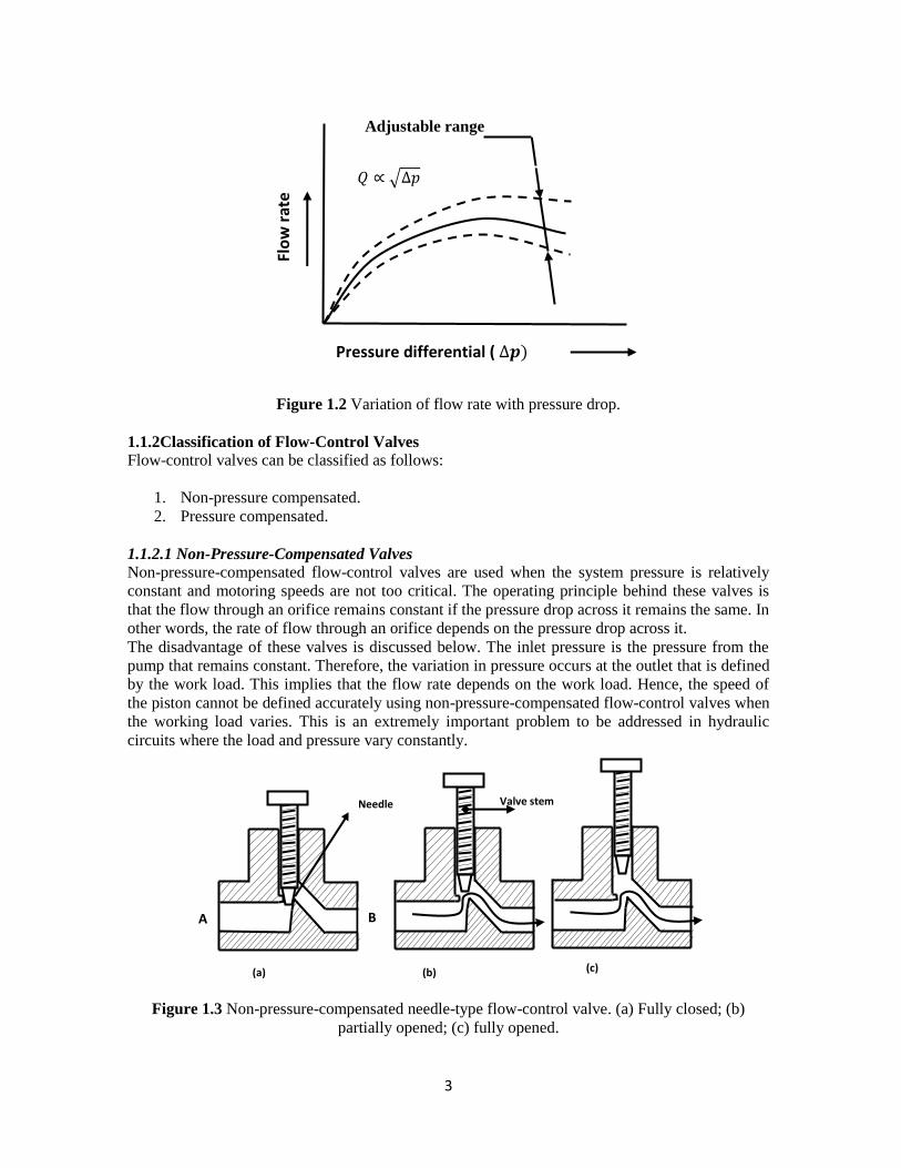
1.1.2.1 Non-Pressure-Compensated Valves

Non-pressure-compensated flow-control valves are used when the system pressure is relatively

constant and motoring speeds are not too critical. The operating principle behind these valves is

that the flow through an orifice remains constant if the pressure drop across it remains the same. In

other words, the rate of flow through an orifice depends on the pressure drop across it.

The disadvantage of these valves is discussed below. The inlet pressure is the pressure from the

pump that remains constant. Therefore, the variation in pressure occurs at the outlet that is defined

by the work load. This implies that the flow rate depends on the work load. Hence, the speed of

the piston cannot be defined accurately using non-pressure-compensated flow-control valves when

the working load varies. This is an extremely important problem to be addressed in hydraulic

circuits where the load and pressure vary constantly.

Figure 1.3 Non-pressure-compensated needle-type flow-control valve. (a) Fully closed; (b)

partially opened; (c) fully opened.

A

(c) (b) (a)

Needle Valve stem

B

Adjustable range

Pressure differential (

Flo

w r

ate

√

4

Schematic diagram of non-pressure-compensated needle-type flow-control valve is shown in Fig.

1.3. It is the simplest type of flow-control valve. It consists of a screw (and needle) inside a tube-

like structure. It has an adjustable orifice that can be used to reduce the flow in a circuit. The size

of the orifice is adjusted by turning the adjustment screw that raises or lowers the needle. For a

given opening position, a needle valve behaves as an orifice. Usually, charts are available that

allow quick determination of the controlled flow rate for given valve settings and pressure drops.

Sometimes needle valves come with an integrated check valve for controlling the flow in one

direction only. The check valve permits easy flow in the opposite direction without any

restrictions. As shown in Fig. 1.4, only the flow from A to B is controlled using the needle. In the

other direction (B to A), the check valve permits unrestricted fluid flow.

Figure 1.4Flow-controlvalve with an integrated check valve.

1.1.2.2Pressure-Compensated Valves

Pressure-compensated flow-control valvesovercome the difficulty causedby non-pressure-

compensated valves by changing the size of the orifice in relation to the changes in the system

pressure. This is accomplished through a spring-loaded compensator spool that reduces the size of

the orifice when pressure drop increases. Once the valve is set, the pressure compensator acts to

keep the pressure drop nearly constant. It works on a kind of feedback mechanism from the outlet

pressure. This keeps the flow through the orifice nearly constant.

B A B A

Restricted flow Free flow

5

Figure 1.5 Sectional view of a pressure-compensated flow-control valve.

Figure 1.6 Graphic symbol of a pressure-compensated flow-control valve.

Schematic diagram of a pressure compensated flow-control valve is shown in Fig. 1.5 and its

graphical symbol in Fig. 1.6. A pressure-compensated flow-control valve consists of a main spool

and a compensator spool. The adjustment knob controls the main spool’s position, which controls

the orifice size at the outlet. The upstream pressure is delivered to the valve by the pilot line A.

Similarly, the downstream pressure is ported to the right side of the compensator spool through the

pilot line B. The compensator spring biases the spool so that it tends toward the fully open

position. If the pressure drop across the valve increases, that is, the upstream pressure increases

relative to the downstream pressure, the compensator spool moves to the right against the force of

the spring. This reduces the flow that in turn reduces the pressure drop and tries to attain an

equilibrium position as far as the flow is concerned.

In the static condition, the hydraulic forces hold the compensator spool in balance, but the bias

spring forces it to the far right, thus holding the compensator orifice fully open. In the flow

condition, any pressure drop less than the bias spring force does not affect the fully open

compensator orifice,but any pressure drop greater than the bias spring force reduces the

compensator orifice. Any change in pressure on either side of the control orifice, without a

corresponding pressure change on the opposite side of the control orifice, moves the compensator

spool. Thus, a fixed differential across the control orifice is maintained at all times. It blocks all

flow in excess of the throttle setting. As a result, flow exceeding the preset amount can be used by

other parts of the circuit or return to the tank via a pressure-relief valve.

Pilot line B

Pilot

line A

Drain

line

A

B Main spool

Compression

spring

Compensator

spool

Adjustment

knob

6

Performance of flow-control valve is also affected by temperature changes which changes the

viscosity of the fluid. Therefore, often flow-control valves have temperature compensation.

Graphical symbol for pressure and temperature compensated flow-control valve is shown in Fig.

1.7.

Figure 1.7Pressure- and temperature-compensated flow-control valve.

1.2Speed-Controlling Circuits

In hydraulic operations, it is necessary to control the speed of the actuator so as to control the

force, power, timing and other factors of the operation. Actuator speed control is achieved by

controlling the rate of flow into or out of the cylinder.

Speed control by controlling the rate of flow into the cylinder is called meter-in control.Speed

control by controlling the rate of flow out of the cylinder is called meter-out control.

1.2.1 Meter-In Circuit

Figure 1.8 shows a meter-in circuit with control of extend stroke. The inlet flow into the cylinder

is controlled using a flow-control valve. In the return stroke, however, the fluid can bypass the

needle valve and flow through the check valve and hence the return speed is not controlled. This

implies that the extending speed of the cylinder is controlled whereas the retracing speed is not.

Figure 1.8Meter-in circuit.

CV FCV

7

1.2.2 Meter-Out Circuit

Figure 1.9 shows a meter-out circuit for flow control during the extend stroke. When the cylinder

extends, the flow coming from the pump into the cylinder is not controlled directly. However, the

flow out of the cylinder is controlled using the flow-control valve (metering orifice). On the other

hand, when the cylinder retracts, the flow passes through the check valve unopposed, bypassing

the needle valve. Thus, only the speed during the extend stroke is controlled.

Both the meter-in and meter-out circuits mentioned above perform the same operation (control the

speed of the extending stroke of the piston), even though the processes are exactly opposite to one

another.

Figure 1.9 Meter-Out circuit.

1.2.3 Bleed-Off Circuit

Compared to meter-in and meter-out circuits, a bleed-off circuit is less commonly used. Figure

1.10 shows a bleed-off circuit with extend stroke control. In this type of flow control, an additional

line is run through a flow-control valve back to the tank. To slow down the actuator, some of the

flow is bledoff through the flow-control valve into the tank before it reaches the actuator. This

reduces the flow into the actuator, thereby reducing the speed of the extend stroke.

The main difference between a bleed-off circuit and a meter-in/meter-out circuit is that in a bleed-

off circuit, opening the flow-control valve decreases the speed of the actuator, whereas in the case

of a meter-in/meter-out circuit, it is the other way around.

FCV

QFCV

CV

8

Figure 1.10 Bleed-off circuits:(a) Bleed-off for both directions and (b) bleed-off for inlet to the

cylinder or motor.

Example 1.1

A 55-mm diameter sharp-edged orifice is placed in a pipeline to measure the flow rate. If the

measured pressure drop is 300 kPa and the fluid specific gravity is 0.90, find the flow rate in units

of 3m /s .

Solution: For a sharp-edged orifice, we can write

V0.0851   SG

pQ AC

where Q is the volume flow rate in LPM,VC is the capacity coefficient = 0.80 for the sharp-edge

orifice, c = 0.6 for a square-edged orifice, A is the area of orifice opening in mm2, p is the

pressure drop across the orifice (kPa) and SG is the specific gravity of the flowing fluid = 0.9.

Now,

2 2 2

orifice  orifice( ) (55 ) 2376 mm4 4

A D

Using the orifice equation we can find the flow rate as

300(LPM) 0.0851 2376  0.80 

0.9Q

= 2953.3 LPM = 0.0492 3 m /s

PRV

PRV

(b) (a)

9

Example 1.2

For a given orifice and fluid, a graph can be generated showing a p versus Q relationship. For

the orifice and fluid in Example 1.1, plot the curves and check the answers obtained

mathematically. What advantage does the graph have over the equation? What is the disadvantage

of the graph?

Solution: From Example 1.1, we have

300

(LPM) 0.0851 2376  0.80 0.9

Q

We can write the general expression as

(LPM) 0.0851 2376 0.80    161.76  170.50.9 0.9

p pQ

p

Using Excel, the graph shown in Fig. 1.11 is obtained.

Figure 1.11 Pressure drop versus flow rate.

From the graph, corresponding to 300 kPa,  p we get Q = 2950 LPM which is close to 2953.3

LPM.A graph is quicker to use but is not as accurate as the equation. A pressure gauge can be

calibrated (according to this relationship) to read Q directly rather than p .

Example 1.3

Determine the flow rate through a flow-control valve that has a capacity coefficient of

2.2LPM/ kPa  and a pressure drop of 687 kPa. The fluid is hydraulic oil with a specific gravity of

0.90.

Solution:For a sharp-edged orifice, we can write

687

2.2 2.2 60.8 LPMSG 0.9

pQ

0

50

100

150

200

250

300

350

400

450

0 500 1000 1500 2000 2500 3000 3500 4000

Pre

ssu

re d

rop

(kP

a)

Flow rate (LPM)

10

Example 1.4

The system shown in Fig. 1.12 has a hydraulic cylinder with a suspended load W. The cylinder

piston and rod diameters are 50.8 and 25.4 mm, respectively. The pressure-relief valve setting is

5150 kPa. Determine the pressure p2 for a constant cylinder speed:

(a) W = 8890 N

(b) W = 0 ( load is removed)

(c) Determine the cylinder speeds for parts (a) and (b) if the flow-control valve has a

capacity coefficient of 0.72LPM/ kPa  . The fluid is hydraulic oil with a specific gravity

of 0.90.

Figure 1.12 Hydraulic cylinder with a suspended weight.

Solution:

For a constant cylinder speed, the summation of the forces on the hydraulic cylinder must be equal

to zero. Thus, we have

1 p 2 p r( ) 0W p A p A A

where 1 pressure-relief valve setting 5150 kPap . Now

W

11

2 2 2

p  P           ( ) (0.0508 ) 0.00203 m4 4

A D

2 2 2

r  R           ( ) (0.0254 ) 0.000506 m4 4

A D

So

2

p r             0.00152  mA A

Case 1: If W = 8890 N.

1 p 2 p r( ) 0W p A p A A

3 3 2 2

2

28890 5150 10 2.0N 3 10 m (0.00152 m ) 0/m p

2

28890 10450 m (0.00152) 0p

2 12700 kPap

Case 2: If W = 0.

3 3 2 2

2

20 5150 10 2.03 10 m (0.001N 52m m ) 0/  p

2 6880 kPap

Case 3: Cylinder speed for case 1: For a sharp-edged orifice, we can write

V

127000.72 85.5 LPM

SG 0.9

pQ C

where2p p because the flow-control valve discharges directly to the oil tank. This is the flow

rate through the flow-control valve and thus the flow rate of the fluid leaving the hydraulic

cylinder. Thus, we have

p p r( )v A A Q

3

2

p 3

1 m 1 min(m/s)(0.00152) m 85.5  L/min

10 L 60 sv

p 0.938  m/sv

Case 4: Cylinder speed for case 2. We have

3 3

V 3

6880 1 m 1 min m0.72 63 LPM=63 L/min 0.00105

SG 0.9 10 L 60 s

pQ C

s

Also we can write

p

3

Velocity×Area

m0.00105

Q

v A

s

2

p (m/s)(0.00152) m 0.00105v

p 0.691  m/sv

Example 1.5

A cylinder has to exert a forward thrust of 100 kN and a reverse thrust of 10 kN. The effects of

using various methods of regulating the extend speed will be considered. In all the cases, the

retract speed should be approximately 5 m/min utilizing full pump flow. Assume that the

12

maximum pump pressure is 160 bar and the pressure drops over the following components and

their associated pipe work (where they are used):

Filter = 3 bar

Directional control valve (DCV) = 2 bar

Flow-control valve (controlled flow) = 10 bar

Flow-control valve (check valve) = 3 bar

Determine the following:

(a) The cylinder size (assume the piston-to-rod area ratio to be 2:1).

(b) Pump size.

(c) Circuit efficiency when using the following:

Case 1: No flow controls (calculate the extend speed).

Case 2: Meter-in flow control for extend speed 0.5 m/min.

Case 3: Meter-out flow control for extend speed 0.05 m/min.

Solution:

Case 1: No flow controls (Fig. 1.13)

Part (a) No flow controls

Maximum available pressure at the full bore end of cylinder = 160 − 3 − 2 = 155 bar

Back pressure at the annulus side of cylinder = 2 bar.

This is equivalent to 1 bar at the full bore end because of the 2:1 area ratio. Therefore, the

maximum pressure available to overcome load at the full bore end is 155 − 1 = 154 bar

Full bore area = Load/Pressure = 100  1  03

1  54  1  05

=0.00649 m

2

Piston diameter = 1/2

4   0.00649

Select a standard cylinder, say with 100-mm bore and 70-mm rod diameter. Then

Full bore area = 7.85 × 103

m2

Annulus area = 4.00 × 103

m2

This is approximately a 2:1 ratio.

Part (b)No flow controls

Flow rate for a return speed of 5 m/min is given by

Area × Velocity = 4.00 × 103

× 5 m3/min = 20 LPM

Extend speed = 3

3

20  10

7.85  10

= 2.55 m/min

Pressure to overcome load on extend = 3

3

100  10

7.85  10

= 12.7 MPa = 127 bar

Pressure to overcome load on retract =

3

3

10  10

4.00  10

= 2.5 MPa = 25 bar

13

(i) Pressure at pump on extend (working back from the DCV tank port)

Pressure drop over DCV B to T 2 × (1/2) 1

Load-induced pressure 127

Pressure drop over DCV P to A 2

Pressure drop over filter 3

Therefore, pressure drop required at the pump during extend stroke = 133 bar

Relief-valve setting = 133 + 10% = 146 bar

(ii) Pressure required at the pump on retract (working from the DCV port as before) is

(2 × 2) + 25 + 2 + 3 = 34 bar

Note: The relief valve will not be working other than at the extremities of the cylinder stroke.

Also, when movement is not required, pump flow can be discharged to the tank at low pressure

through the center condition of the DCV.

Part (c) No flow controls System efficiency:

Energy required to overcome load on the cylinder Flow to the cylinder   Pressure owing to load

Total energy into fluid Flow from the pump   Pressure at the pump

Efficiency on extend stroke = 20  1  27

20  1  33

× 100 = 95.5 %

Efficiency on retract stroke = 20   25 

20   34

× 100 = 73.5 %

14

Figure 1.13 Hydraulic cylinder with no control.

Case 2: Meter-in flow control for the extend speed of 0.5 m/min(Fig. 1.14)

Part (a) meter in controls

From case 1,

Select a standard cylinder, say with 100-mm bore and 70-mm rod diameter.

Cylinder 100-mm bore diameter × 70-mm rod diameter

Full bore area 7.85 × 10–3

m2

Annulus area = 4.00 × 10–3

m2

Load-induced pressure on extend = 127 bar

Load-induced pressure on retract = 25 bar

Pump flow rate = 20 L/min

Part (b) meter in controls

Flow rate required for the extend speed of 0.5 m/min is

7.85 × 10–3

× 0.5= 3.93 × 10–3

m3/min = 3.93 L/min

Working back from the DCV tank port:

Pressure required at the pump on retract is

(2 × 2) + (2 × 3) + 25 + 2 + 3 = 40 bar

Pressure required on the pump at extend is

2 × (1/2) + 127 + 10 + 2 + 3 = 143 bar

Relief-valve setting = 143 + 10% = 157 bar

This is close to the maximum working pressure of the pump (160 bar). In practice, it would be

advisable to select either a pump with a higher working pressure (210 bar) or use the next standard

15

size of the cylinder. In the latter case, the working pressure would be lower but a higher flow rate

pump would be necessary to meet the speed requirements.

Part (c) meter in controls

Now that a flow-control valve has been introduced when the cylinder is on the extend stroke, the

excess fluid will be discharged over the relief valve.

System efficiency on extend = 3.93  1  27

20  1  57

× 100 = 15.9%

System efficiency on retract =    20   25

20   40

1  00 = 62.5%

Figure 1.14 Hydraulic cylinder with meter-in control

Case 3: Meter-out flow control for the extend speed of 0.5 m/min(Fig. 1.15)

Cylinder, load, flow rate and pump details are as before (partsa and b of meter in control).

Part (c) meter out controls

Working back from the DCV tank port:

16

Pressure required at the pump on retract is

(2 × 2) + 25 + 3 + 2 + 3 = 37 bar

Pressure required at the pump on extend is

[2 ×(1/2)] + [10 × (1/2)] + 127 + 2 +3 = 138 bar

Relief-valve setting = 38 + 10 % = 152 bar

System efficiency on extend = 3.93  1  27

20  1  52

× 100 = 16.4%

System efficiency on retract =   20   25

20   37

× 100 = 67.6%

Discussion of results of all three cases: No control, meter-in and meter-out.

As can be seen, meter-out is marginally more efficient than meter-in owing to the ratio of piston to

piston rod area. Both systems are equally efficient when used with through-rod cylinders or

hydraulic motors. It must be remembered that meter-out should prevent any tendency of the load

to run away.

In both cases, if the system runs light, that is, extends against a low load, excessive heat is

generated over the flow controls in addition to the heat generated over the relief valve.

Consequently, there is further reduction in the efficiency. Also, in these circumstances, with

meter-out flow control, very high pressure intensification can occur on the annulus side of the

cylinder and within the pipe work between the cylinder and the flow-control valve. Take a

situation where meter-out circuit is just considered. The load on extend is reduced to 5 kN without

any corresponding reduction in the relief-valve settings.

Flow into the full bore end is 3.91 L/min.

Therefore, excess flow from the pump is

20 – 3.93= 16.07 L/min

that passes over the relief valve at 152 bar.

The pressure at the full bore end of the cylinder is = 152 – 3 – 2 = 147 bar

This exerts a force that is resisted by the load and the reactive back pressure on the annulus side:

147 –

3

3 5

           5  10

7.85  1  0 1  0

= (2 + 10 + p) ×

4.00

7.85

wherep is the pressure within the annulus side of the cylinder and between the cylinder ant the

flow-control valve. So

p = [(147 – 6.4) × 7.85/4.00] – 12 = 264 bar

The system efficiency on extend is

 3.93   6.4  

20  1  52 

× 100 = 0.83%

Almost all of the input power is wasted and dissipates as heat into the fluid, mainly across the

relief and flow-control valves.

17

Figure 1.15 Hydrauliccylinder with meter-out control.

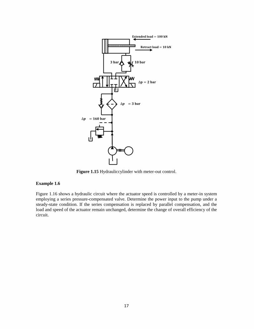
Example 1.6

Figure 1.16 shows a hydraulic circuit where the actuator speed is controlled by a meter-in system

employing a series pressure-compensated valve. Determine the power input to the pump under a

steady-state condition. If the series compensation is replaced by parallel compensation, and the

load and speed of the actuator remain unchanged, determine the change of overall efficiency of the

circuit.

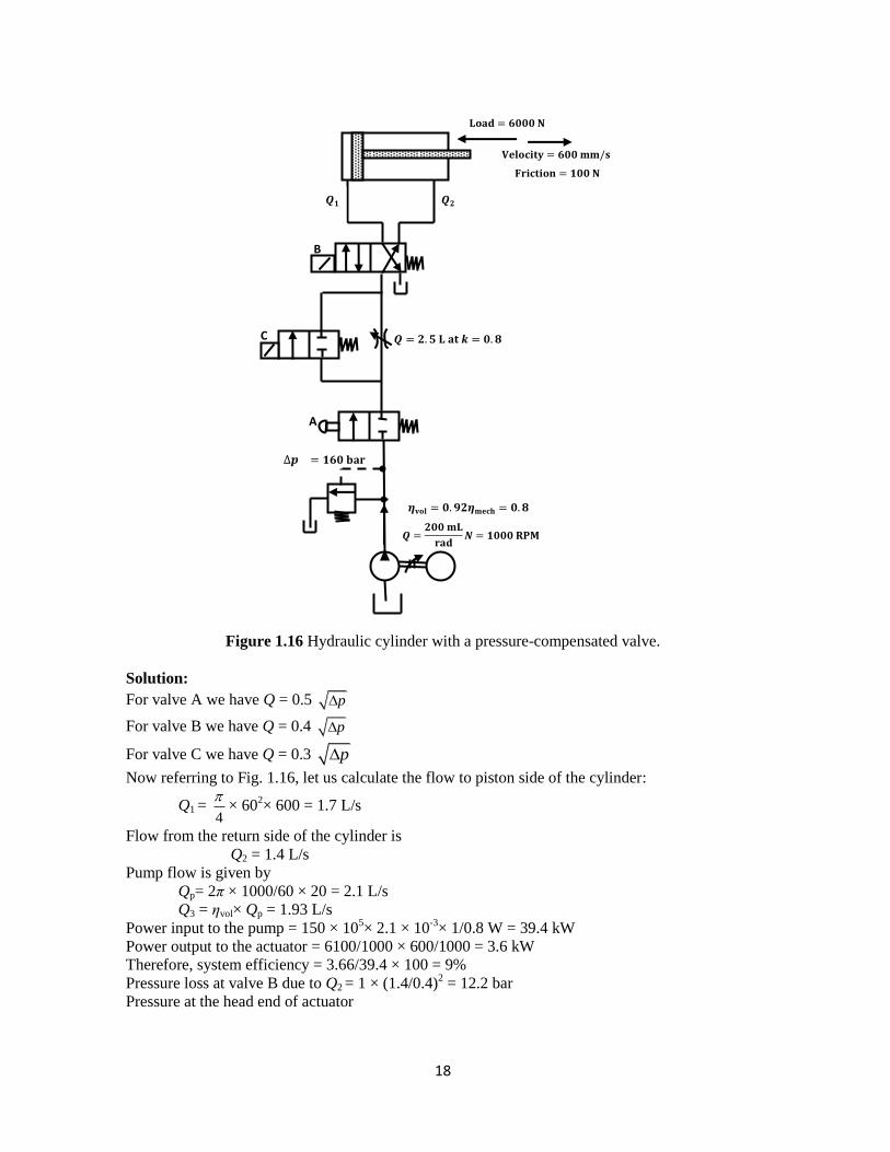
18

Figure 1.16 Hydraulic cylinder with a pressure-compensated valve.

Solution:

For valve A we have Q = 0.5 p

For valve B we have Q = 0.4 p

For valve C we have Q = 0.3 p

Now referring to Fig. 1.16, let us calculate the flow to piston side of the cylinder:

Q1 = 4

× 60

2× 600 = 1.7 L/s

Flow from the return side of the cylinder is

Q2 = 1.4 L/s

Pump flow is given by

Qp= 2π × 1000/60 × 20 = 2.1 L/s

Q3 = ηvol× Qp = 1.93 L/s

Power input to the pump = 150 × 105× 2.1 × 10

-3× 1/0.8 W = 39.4 kW

Power output to the actuator = 6100/1000 × 600/1000 = 3.6 kW

Therefore, system efficiency = 3.66/39.4 × 100 = 9%

Pressure loss at valve B due to Q2 = 1 × (1.4/0.4)2 = 12.2 bar

Pressure at the head end of actuator

A

B

C

19

p ×4

× 60

2× 10

–6 = 6100 + 12.2 × 10

5 ×

4

× (602 – 252) × 10

–6

p = 29 bar

Pressure losses at B due to Q1 = (1.7/0.4)2 = 18 bar

Pressure losses at valve A = (1.7/0.5)2 = 11.6 bar

Therefore, the total pressure, excluding that lost in the pressure-compensated valve if it is of series

type, is

29 + 18 + 11.6 + 4 = 62.6 bar

Hence, 150 – 62.6 = 87.4 bar is dropped in the pressure-compensated valve if it is of series type.

For a parallel pressure-compensated valve, the excess oil Q – Q1 would bypass at

62.6 bar – 11.6 bar = 51 bar

The pump delivery would be at 62.6 bar and hence the total power consumption is

62.6 × 105× 2.1 × 10

3× 1/0.8 W = 16.5 kW

System efficiency = 22.2%

Example 1.7

A flow-control valve is used to control the speed of the actuator as shown in Fig. 1.17 and the

characteristics of the system are given in Table 1.1. Determine the variable flow area Av, the

pressure downstream of the valve fixed orifice p2, the valve displacement x and the spring preload

F for the given motor operating conditions.

Table 1.1

Parameters Value

Valve flow constant (d )C 0.6

Length h 7.8 mm

Valve area gradient for flow area (

vA ), b

1.25 mm2/mm

Fixed orifice flow area (o )A 4.9 mm

2

Valve face area (A) 125 mm2

Spring constant 57 kN/m

Motor displacement (m )D 40 cm

3/rev

Motor torque 60 Nm

Motor speed 350 RPM

Motor volumetric efficiency (v ) 96 %

Motor mechanical efficiency (m ) 97 5

20

System pressure (1)p 14.5 MPa

Return pressure (4 )p 1 MPa

Fluid density 840 kg/m3

Figure 1.17

Solution: Refer to Fig. 1.17, flow from the pump divides as 1Q and

2Q . The pressure drop 1 2p p

occurs across orifice Ao. This makes the valve to move to right against the spring force F. The area

of orifice Av then adjusts to control the flow to the motor:

Let us first convert all the given variables to appropriate units

6 2 6 2

o

7.8 1.25  m,    mm,      57000 N/m,    4.9 1  0 m    1  25 10 m

1000 100,

0

   

h w k A A

3

33 2

m 1̀

40m

100  ,    60 N m,   350 RPM,     840 kg/m , 145000 1000 N/mrev

  

D T n p

V m `4

2 350  96%,     97%,   1000 1000 Pa, 36.652 rad/s

60p

First let us calculate the discharge 2  Q through valve

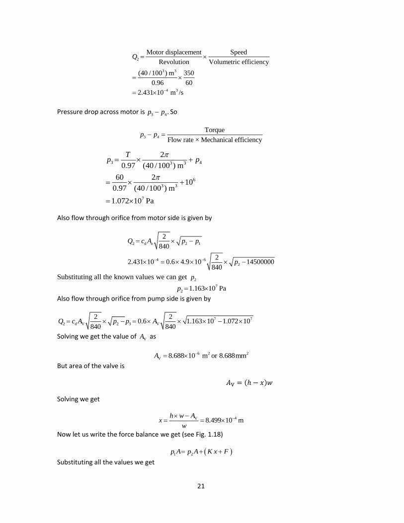
21

2

3 3

4 3

Motor displacement Speed 

Revolution Volumetric efficiency

(40 /100 m 350 

0.96 60

2.431  1  0 m /s

)

Q

Pressure drop across motor is3 4  .p p So

3 4

Torque 

Flow rate × Mechanical efficiencyp p

3 43 3

6

3 3

7

2   

0.97 (40 /100 ) m

60 210

0.97 (40 /100 ) m

1.072  1  0  Pa

Tp p

Also flow through orifice from motor side is given by

2 d o 2 1

4 6

2

2   

840

22.431  10 0.6 4.9 10 14500000

840

Q c A p p

p

Substituting all the known values we can get 2p

7

2   1.163  1  0  Pap

Also flow through orifice from pump side is given by

2 d V 2 3 V

7 72 2   

840 840.6 1.163 10 1.072 10

0Q c A p p A

Solving we get the value of VA as

6 2 2

V 8.688  10 m  or  8.688  mmA

But area of the valve is

(

Solving we get

4V 8.499  10  mh w A

xw

Now let us write the force balance we get (see Fig. 1.18)

1 2       p A p A K x F

Substituting all the values we get

22

2 6 7 6 414500 1000 N/m 125 10   1.163  1  0 125 10 57000  8.499  10   F

310.4 NF

Figure 1.18

A

23

Objective-Type Questions

Fill in the Blanks

1. Non-pressure-compensated flow-control valves are used when the system pressure is relatively

________ and motoring speeds are not too critical.

2. A pressure compensator acts to keep the ________ nearly constant.

3. In ________ flow-control valve consists of a main spool and a compensator spool.

4. Speed control by controlling the rate of flow ________ the cylinder is called meter-in control.

5. In a meter-________ circuit, only the speed during the extend stroke is controlled.

State True or False

1. The speed of a piston can be defined accurately using non-pressure-compensated flow-control

valves when the working load varies.

2. Speed control by controlling the rate of flow out of the cylinder is called meter-in control.

3. In a meter-in circuit, the extending speed of the cylinder is controlled whereas the retracing

speed is not.

4. Compared to the meter-in and meter-out circuits, the bleed-off circuit is more commonly used.

5. In a meter-in circuit, flow coming from the pump into the cylinder is not controlled directly.

However, the flow out of the cylinder is controlled using a flow-control valve.

Review Questions

1. What is the function of a flow-control valve?

2. What are the three ways of applying flow-control valves?

3. What is meant when a flow-control valve is said to be pressure compensated?

4. What is a meter-in circuit and where is it used?

5. What is a meter-out circuit and where is it used?

6. What are the advantages of a meter-in circuit?

7. What are the disadvantages of a meter-in circuit?

8. What are the advantages of a meter-out circuit?

9. What are the disadvantages of a meter-out circuit?

10. What are the advantages of a by-pass or bleed-off circuit?

11.What are the disadvantages of a by-pass or bleed-off circuit?

12. What is a modular valve and what are its benefits?

13. What is a hydraulic fuse?

14.What is the need for temperature compensation in a flow-control valve?

15. What is the difference between a hydraulic fuse and a pressure-relief valve?

24

Answers

Fill in the Blanks

1.Constant

2.Pressure drop

3.Pressure compensated

4.Into

5.Out

State True or False

1.False

2.False

3.True

4.False

5.False