processes

Article

Dynamic Semi-Quantitative Risk Research inChemical Plants

Qiusheng Song 1, Peng Jiang 1,*, Song Zheng 1, Yaguang Kong 1, Ye Zhao 2 and Gang Shen 3

1 Department of Control Science and Engineering, Hangzhou Dianzi University, Hangzhou 310018, China;songqiusheng@hdu.edu.cn (Q.S.); zhs@hdu.edu.cn (S.Z.); ygkong@hdu.edu.cn (Y.K.)

2 Quzhou Special Equipment Inspection Center, Quzhou 324000, China; zhaoye0123@sina.com3 Zhejiang Transit Fluorine Silicon Limited Company, Quzhou 324000, China; shengang1121@sina.com* Correspondence: pjiang@hdu.edu.cn

Received: 26 August 2019; Accepted: 8 November 2019; Published: 12 November 2019�����������������

Abstract: When a major accident occurs in a chemical industry park, it directly affects the personalsafety of operators and neighboring residents and causes major losses; therefore, we should takemeasures to strengthen the management of chemical industry parks. This article proposes andanalyzes a new dynamic semi-quantitative risk calculation model for chemical plants that can beapplied digitally. This model provides a sustainable, standardized, and comprehensive managementstrategy for the safety management of chemical plants and chemical industry park managers.The model and its determined parameters were applied to the safety management of chemicalcompanies within the chemical industry park of Quzhou, Zhejiang Province. From the point of viewof the existing semi-quantitative model, the existing problems of the current model are analyzed,the current model is optimized, and a new dynamic semi-quantitative calculation model scheme isproposed. The new model uses an analytical hierarchy process targeting the factors affecting the risksin chemical plants, and chemical plant semi-quantitative dynamic calculation system consisting ofthe operator, process/equipment, risk, building environment, safety management, and domino effect,and the comprehensive risk of the chemical plant was calculated. The model is ultimately a real-timequantitative value, but its calculation process can compare and analyze the causes of high risk in achemical plant as they relate to these six factors. Its implementation requires only software, whichwill greatly help chemical plant safety management.

Keywords: analytical hierarchy process; chemical plants; dynamic semi-quantitative calculation;risk value

1. Introduction

Chemical industry parks are built in development zones and are based on the development ofoil and chemicals. They have unique inner features, and their most important characteristic is thatthey are potentially dangerous. Due to the nature of chemical products, chemical industrial parksare potentially high risk: chemical plants are concentrated in the parks, and there are many majorhazards such as inflammable, explosive, and toxic chemicals within them. When an accident occurs,the consequences can be very serious. Historical examples include the Bhopal tragedy [1], the PiperAlpha [2], the Flixborough disaster [3], BP Texas City [4], the West Fertilizer explosion [5], the Tianjinexplosion, etc. [6] (details of these events are shown in Table 1).Therefore, the safety management ofchemical industry parks is very important.

Processes 2019, 7, 849; doi:10.3390/pr7110849 www.mdpi.com/journal/processes

Processes 2019, 7, 849 2 of 28

Table 1. Some major chemical accidents in recent years.

Time Accident Location Accident Type Death Toll Direct Property Loss

1974.6.1 Flixborough Chemical explosion 28 unknown1984.12.2 Bhopal Chemical poisoning 25,000 $470 million1988.7.6 Piper Alpha Chemical explosion 167 $7500 million

2013.4.17 State of Texas Chemical explosion 35 unknown2015.8.12 Binhai, Tianjin Chemical explosion 165 $1098 million

To prevent and control major chemical safety accidents, we need to take appropriate measures tostrengthen the management of chemical industry parks. There are many factors affecting chemicalsafety accidents, mainly human, machine, material, method, environment, management, and others;if we can comprehensively monitor and manage these safety factors, we can detect potential safetyproblems in a timely manner and immediately rectify and improve them to prevent major accidents.Targeted management of the risk level of dangerous chemicals in chemical industry parks can beused to fully mobilize the limited resources of government departments and plants. The focus ofsuch management, rational distribution, is one of the most ideal management tools currently used inchemical industry parks. Therefore, chemical industry parks should implement a combination of keymanagement of major chemical hazards and real-time monitoring.

Comparatively more research has been invested in hazard risk assessment, and quantitative riskassessment methods have been used in the overall risk assessment and safety planning of chemicalindustry parks, for example, the U.K.’s Canvey Island research project in 1978, Italy’s Ravenna researchproject in 1979, and the Rijnmond research project in the Netherlands in 1979 [7]. In 2002, the EuropeanUnion research center launched the ARAMIS(accidental risk assessment methodology for industries)project and provided a comprehensive evaluation system [8,9] as a part of this project. In 2004, Khan F.I,Amyotte P.R proposed the comprehensive essential safety index (I2SI), which consists of two mainsub-indices: the risk index (HI) and the underlying safety potential index [10]. Khakzad et al. [11]applied bow-tie and Bayesian network methods in conducting quantitative risk analysis of drillingoperations. Abimbola et al. [12] performed safety and risk analysis of a managed pressure drillingoperation using Bayesian networks. Goerlandt et al. [13] presented a review focusing on the validationof QRA (quantitative risk analysis) in a safety context. Valerie DE Dianous et al. [14] studied theconsequences and causes of all kinds of accidents faced by plants in the chemical industry andemphasized the use of the bow structure diagram method. Christian Delvosalle et al. [15] analyzedthe possible accident scenarios for various major hazards. Bahman [16] proposed a new approach,which can predict and assess the impact of an accident in one process unit on the other process unitsthat could be affected. Jonkman S.N et al. [17] gave a model of quantitative risk measures for loss oflife and economic damage. Selvik J.T et al. presented and discussed the RCM (reliability centeredmaintenance) framework to improve risk and uncertainty assessments. The QRA techniques used arebased on standard methods, such as fault tree and event tree analysis, but also on more tailor-mademethods and approaches to meet the great diversity of processes, hazardous materials, equipmenttypes, and control schemes that characterize the chemical processing industry [18–20]. In chemicalrisk research, governments are constantly exploring the best ways to solve problems via collaboration.Control standards and procedures related to major hazards are promulgated by the United Kingdom,France, the Netherlands, etc. [21–25]. In terms of risk criteria, Kletz [7] proposed that the highest riskof death among residents in the vicinity of chemical facilities is 10−6 per year, and some companiesin the United Kingdom, the United States, and Denmark use this risk standard. According to therisk assessment methods of major hazards and different occasions, the Dutch government has alsoestablished reference values for personal and social risks relating to chemical plants [26,27]. A riskindex was devised to allow the assessment of the risk level originating from a given installation orsite over the affected zone, and a Bayesian network methodology was developed to estimate the totalprobability of a major accident in a chemical plant [28–32]. The current research detailed above, which

Processes 2019, 7, 849 3 of 28

is mainly used for chemical industry park planning and analysis, cannot be easily used for the dynamicsafety management of existing chemical industry parks; in addition, only the main hazards themselveswere considered in these studies, and other major factors that affect safety accidents, such as human,machine, material, method, and environment, were not considered.

To sum up, there are more mature safety assessment methods that have been developed at homeand abroad, but these are mainly relatively static assessment methods for the planning of chemicalindustry parks. For example, Nancy Leveson [33] presented a new accident model founded onbasic systems theory concepts. The use of such a model provides a theoretical foundation for theintroduction of new unique types of accident analysis, hazard analysis, and accident preventionstrategies. Nancy Leveson [34] also described a new method for identifying system-specific leadingindicators based on the accident causal relationship of the STAMP (System-Theory Accident Modeland Process) model and tools that were intended to be built on the model. There are fewer methodsof dynamic assessment generally, and they do not take into account factors beyond the hazardsthemselves, such as the dynamic process of change in the production and storage of hazards or thecombined effects of operators, process, equipment, the building environment, safety management,and the domino effect [35]. The question that remains, and which we address in this paper, is how tocarry out dynamic and quantitative assessment of the major hazards in a chemical industry park andprovide an assessment result of the dangers in the chemical plants to the park managers promptly andintuitively, so that the park managers can detect the potential safety hazards in time and avoid theoccurrence of major safety accidents. The six influencing factors of the model are all dynamic, andeach inspection time point has a comprehensive quantitative value. The dynamic form can ensure thatthe calculated risk value is a real-time quantitative value, which is in line with the actual situation onsite and ensures that this research will have great practical significance.

Therefore, this article is based on the research of dynamic semi-quantitative real-time monitoringand management methods for major hazards in chemical industry parks as they relate to the operators,process/equipment, risk, building environment, safety management, and domino effect. We analyzeand calculate these six factors and give a dynamic semi-quantitative calculation model of chemicalhazards based on an analytical hierarchy process [36]. Using this model, the risk value of each chemicalplant in a park can be accurately calculated, and the safety hazards of each chemical plant can be foundaccording to the risk value. Our focus is on the improvement and tracking of safety hazards to reducethe probability of accidents.

2. Using the Analytical Hierarchy Process to Establish a Dynamic Semi-Quantitative Evaluation Model

At present, the mature safety evaluation model is based on the R value. This model only considersthe four parameters of the existence of dangerous chemicals (storage) in the major hazards identificationof dangerous chemicals (GB18218) specified in the critical mass, which dangerous chemicals these are,the correction coefficient, and the corresponding correction coefficient of major hazards to which thefactory personnel are exposed. For a chemical plant in a chemical industrial park, other influencefactors, such as the huge number and dense distribution of different kinds of chemical hazards in thepark, make it easier for an accident to cause a domino effect. The risk, operators, processes/equipment,building environment, safety management, and other factors in the chemical plant have a great impacton the risk value of the chemical plant. Therefore, we used an AHP (analytical hierarchy process)to conduct dynamic semi-quantitative assessment and monitoring of hazards in chemical plants.At the same time, the influence of the five factors operator, process/equipment, building environment,safety management, and domino effect was added, and the risk value R’ of the danger source wascomprehensively calculated. The description of the letters used in the equations in this section isshown in Table 2.

Processes 2019, 7, 849 4 of 28

Table 2. Parameters of the dynamic semi-quantitative evaluation model of chemical hazards.

Parameters:

(1) Hazards calculation parameter

R risk valueq1,q2, . . . , qn The actual quantity (in storage) of each dangerous chemical (tons)Q1,Q2, . . . , Qn Corresponding critical mass (ton)β1,β2 . . . , βn The corresponding correction coefficientα Correction factor for number of exposed personnelR3 R value after optimizationR1 Hazards in the production processR2 Hazards of the storage tankq1’,q2’, . . . , qn’ Quantity of each dangerous chemical online (ton)Q1’,Q2’, . . . , Qn’ Corresponding critical mass (ton)

(2) The domino effect calculation parameter

∆p Blast overpressure (Pa)p0 Atmospheric pressure (101,325 Pa)Z Dimensionless distanceL The horizontal distance from the target to the source of the blast (m)E The total explosive energy source (J)α’ Equivalent coefficient for vapor cloud, generally 0.04W1 The mass of fuel in the vapor cloud that actually contributes to the blast shockwave (Kg)QC Heat of combustion of the fuel (J/Kg)q (r) Radiation flux to the target (W/m2)

q0 Radiation flux on the surface of the fireball, cylindrical tank to take 270 kW/m2, spherical tank to take 200 kW/m2

R0 Fireball radius (m)r The horizontal distance from the target to the center of the fireball (m)W2 Fireball consumption of combustible material (kg)t Fireball duration (s)P Domino effect probabilityY Domino effect probability unitt’ No-fault timeI Radiation intensity on the target (KW/m2)V Equipment volume (m3)Pblast The domino effect probability of shockwavePheat The domino effect probability of heat radiationγ Domino coefficient

(3) The operator calculation parameter

H1 Personnel qualifying valueH2 Personnel proficiency valuet2 Staff working time at a postK2 Skilled scale factorT2 The time required to reach a certain level of proficiencyH3 Personnel stability valuet3 Working hours at the postK3 Stability ratio coefficientT3 The time it takes for a person to reach a certain level of operational stability after an accidentH4 Personnel workload valuet4 Personnel work time from work start to work endK4 Workload ratio factorT4 Job normal working-class work time, generally taken to be 8 hM0 Jobs required for the number of workersN0 The actual number of jobs at the post, and N0 < M0H5 The reliability value of a single personHs The reliability of the designated postHp The reliability of a single staff memberHu The reliability of unit personnel quality

(4) The process/equipment, building environment, and safety management calculation parameter

D Process/equipment basic scoreXi The result of process/equipment judgment, yes is 1, no 0E Building environment basic scoreYi The result of building environmental judgment, yes is 1 and no is 0F Safety management basic scoreZi The result of safety management judgment, yes is 1 and no is 0

Processes 2019, 7, 849 5 of 28

2.1. Establishing a Dynamic Semi-Quantitative Risk Calculation Model for Chemical Hazards

In view of the difficult problem of chemical hazard risk assessment, the fishbone diagram analysismethod was used to acquire the six factors that impact the hazard risk, and the six factors wereused to construct the model using the analytical hierarchy process. Then, we confirmed the detailedcalculation of each indicator on the model, used the forced pair comparison to confirm the weightof each factor, and finally produced the dynamic semi-quantitative hazard risk calculation model, asshown in Figure 1.

Figure 1. Flowchart for establishing a dynamic semi-quantitative risk calculation model for chemical hazards.

2.2. Dynamic Semi-Quantitative Calculation and Analysis of Hazards

2.2.1. Dynamic and Quantitative Calculation of Risk Values for Hazards

According to the requirements of the Provisional Regulations on the Supervision andAdministration of Major Dangerous Chemicals, which came into force on 1st, December, 2011,the major hazards are graded by the State Administration of Work Safety (No. 40).

(1) The classification index uses the actual (stored) amounts of various dangerous chemicals in theunit and their critical amount ratios specified in “Identification of Major Hazard of DangerousChemicals” (GB18218); the sum of the ratios of the corrected coefficients is the classification index.

(2) R value calculation

The R value is calculated as shown in Equation (1), which is from the “Identification of MajorHazard of Dangerous Chemicals” (GB18218). From the calculation of the R value, we can see that the Rvalue actually represents the inherent danger of the hazard, which is formulated by coupling betweenaccident proneness and the seriousness of accident consequences. The correspondence between majorhazard levels and R values is shown in Table 3.

R = α

(β1

q1

Q1+ β2

q2

Q2+ . . . . . .+ βn

qn

Qn

)(1)

Processes 2019, 7, 849 6 of 28

Table 3. The levels of significance of chemical hazards and the corresponding R values.

Chemical Hazard Significance Level R Value

Level 1 R ≥ 100Level 2 100 > R ≥ 50Level 3 50 > R ≥ 10Level 4 R < 10

2.2.2. Analysis of Dynamic Semi-Quantitative Hazard Calculation Methods

The R value is currently the traditional classification index for major hazards as it is more intuitive,simple, and easy to calculate; however, its equation does not consider more important factors, only thestorage area of the hazard itself, so it is more suitable for small and medium-sized chemical plants.Chemical plants are more concentrated in chemical parks, and because the R value considers too fewfactors and is not comprehensive enough, it cannot easily reflect all aspects of the characteristics ofchemical industry parks. Thus, we need to increase each influence factor and optimize the R value.Using fishbone chart analysis, we can derive the important factors that most affect the risk value of thehazard, as shown in Figure 2.

Figure 2. Fishbone diagram analysis of the main factors that affect the risk values of chemical hazards.

Hazards in the Pipeline

The current classification of major hazards is calculated based on the stored amount of thehazard in the storage area, which is the main factor affecting the plant risk value. However, hazardsin the pipeline are also a great danger. In the event of an accident, these hazards are also moredestructive, especially in chemical plants where the output of hazards is relatively large. Therefore, inthe calculation of the overall risk value of the chemical plant, this part of the hazards also needs to betaken into account.

Domino Effects in Chemical Industry Parks

The domino effect in a chemical industry park can play an amplifying role in the devastation anddamage caused by an accident. This part is also indispensable in the calculation of the risk value of achemical plant in a chemical park. Valerio Cozzani et al. [35] studied the domino effect in hazards andemphasized the importance of including the domino effect in the calculation of the risk value.

Operator, Equipment, Process, and Environment

“Operator” refers to the operators who use dangerous raw materials and manufacture dangerousproducts; they are the biggest difficulties in production management and are the focus of discussion inall management theories at present. Operators’ personality traits, ability levels, and education levelsare not the same, and their attitude towards the work and awareness of the dangers of the product

Processes 2019, 7, 849 7 of 28

are not the same; all these have a great impact on the safety of the operation. In the past, a majorityof chemical accidents have been due to improper operation by operators. “Equipment” refers to theproduction of machines, tools, and other auxiliary production equipment. In the production process,whether the equipment is functioning or the tools are good or bad is another factor affecting safety.“Process” refers to the documents, regulations, and systems to be followed in the production process,including process instructions, guidelines for standard processes, production drawings, productionschedules, product operating standards, inspection standards, and various operating procedures. If theprocess is wrong, this will result in a major chemical plant accident. “Environment” refers to thebuilding environment, including the layout of the building and temperature and humidity control.The environment also has a great impact on the occurrence of safety incidents, such as sudden changesin temperature and humidity, which may be a direct result of safety incidents, or improper design ofthe building environment, which can amplify the scope of and loss resulting from a safety incident.Therefore, in chemical plant risk factor analysis, the operator, equipment/process, and environmentcannot be ignored.

Safety Management

Safety management is an important part of production management and is a comprehensivesystem of science. The object of safety management is the management and control of the status ofall people, objects, and the environment in production. It is a kind of dynamic management. Safetyand danger exist in the same context in mutual opposition and interdependence. As the movement ofthings changes, safety and danger are changing all the time, and the fight is reversed. The state ofthings will tilt toward the victor of the struggle, showing that there is no absolute safety or danger inthe movement of things. To maintain the safety status of production, we must take various measuresto prevent danger. The risk factors are completely controllable; therefore, in chemical industry parkrisk factor analysis, corporate safety management is also the top priority.

2.3. Analysis of Influencing Factors in the Dynamic Quantitative Evaluation

2.3.1. Increased Risk of Quantities in the Pipeline

Hazards in storage are a major risk for all chemical plants in a chemical industry park and forma major part of the risk value. The sum of all similar hazards stored on site needs to be calculated.In addition, there is also a need to supplement this with the risk value in the production pipeline, asshown in Equations (2) to (4).

R3= R1+R2 (2)

R1 = α

(β1

q1

Q1+ β2

q2

Q2+ . . . . . .+ βn

qn

Qn

)(3)

R2 = α

(β1

q′1Q′1

+ β2q′′2Q′2

+ . . . . . .+ βnq′nQ′n

)(4)

2.3.2. Domino Effect

The calculation of the domino effect coefficient includes two parameters: the probability of shockdomino effect (Pblast) and the probability of thermal radiation domino effect (Pheat). The calculation ofthe domino effect probability was obtained using a simulation evaluation of accident consequences.By selecting the explosion and fire models as the accident consequence models, we can get theshockwave domino effect probability and the thermal radiation domino effect probability; while thereare several accident consequence models for a chemical industry park, the more common are explosionand fire.

(1) Explosion—blast shockwave overpressure

Processes 2019, 7, 849 8 of 28

An explosion is a very sharp physical and chemical change of matter. It is also a phenomenon inwhich a large amount of energy is quickly released or rapidly transformed into mechanical work ina short time. It is usually achieved by means of gas expansion, which can be physical explosion orchemical explosion according to the nature of the explosion. Physical explosion is a phenomenon inwhich the material state parameters (temperature, pressure, and volume) change rapidly and emit largeamounts of energy and work externally in an instant. Chemical change is the rapid transformation of asubstance from one chemical structure to another chemical structure, releasing a large amount of energyand doing work externally. The main types of explosion models are blasting energy from compressedgas containers, blasting energy when all of the media are liquid, blasting energy of liquefied gases, andhigh-temperature saturated water, steam cloud explosions, and shockwave overpressure.

Overpressure on the shockwave front in shockwave overpressure models is related to the ability togenerate shockwaves and is also related to the distance from the explosion center. Shock overpressurecan be calculated as shown in Equations (5) to (7).

∆pP0

= 0.137Z−1 + 0.119Z−2 + 0.269Z−1− 0.019 (5)

Z = L•(P0

E

) 13

(6)

E = 1.8α′W1QC (7)

(2) Fire—thermal radiation

There are two main types of fire assessment: pool fire and vapor explosion (BLEVE).Liquid leaks generally cause pool fire, the damage from which is mainly thermal radiation. If the

heat radiation acts on containers and equipment, especially liquefied gas containers, the internalpressure will rapidly rise, causing the container and equipment to rupture; if heat radiation acts oncombustibles, it ignites them; and if heat radiation is applied to personnel, it can cause burns and death.Vapor explosion refers to the sudden boiling of liquid generated by massive overheating causing anexplosive boiling phenomenon. The BLEVE acronym stands for “boiling liquid expanded to vaporexplosion”, but this is too cumbersome, so it is simplified to “vapor explosion”. According to thecharacteristics of dangerous chemicals in a chemical industry park, we selected the vapor explosion(BLEVE) model. The thermal radiation flux of this model is calculated as shown in Equations (8) to (10).

q(r) =q0R0

2r(1− 0.058lnr)

(R02 + r2)3/2(8)

R0 = 2.9W21/3 (9)

t = 0.45W21/3 (10)

(3) The accident domino effect threshold

In order to judge whether a domino effect will occur after a major accident occurs, thresholdvalues of the relevant physical parameters characterizing the damage effect are generally selected fordetermination. If the calculation result of the related physical parameter exceeds the threshold value,a domino effect is considered to be caused.

a. Thermal radiation domino effect threshold

The threshold of heat radiation for atmospheric pressure vessels over more than 10 min is15 kW/m2, and the threshold for thermal radiation for pressure vessels over more than 10 min is50 kW/m2; these were given by Valerio Cozzani et al. [37]. The setting of these thresholds has beenapproved by other international scholars, and this article also adopts these thresholds.

Processes 2019, 7, 849 9 of 28

b. Shock wave domino effect threshold

Along with the thresholds for the domino effect from thermal radiation, Valerio Cozzani et al. [37]gave destruction thresholds for atmospheric pressure vessels, pressure vessels, long vessels, and smallvessels, respectively, of 22 kPa, 16 kPa, 31 kPa, and 37 kPa. The setting of these thresholds has beenapproved by other international scholars, and this article also adopts these thresholds.

(4) Domino effect probability

The domino effect probability formula calculates the probability of damage to equipment basedon the probability function method for empirical data, as shown in Equation (11). The most commonequipment failure probability models are shown in Table 4.

P =1√

2π

∫ Y−5

−∞

e−x22 dx (11)

Table 4. Commonly used equipment failure probability models.

Physical Factors Container Type Threshold Probability Calculation Equations

Overpressure

Atmospheric pressure 22 kPa Y = −18.96 + 2.44lnPsPressure 16 kPa Y = −42.44 + 4.33lnPs

Long type 31 kPa Y = −28.07 + 3.16lnPsSmall type 37 kPa Y = −17.79 + 2.18lnPs

Heat radiationAtmospheric pressure More than 10 m,15 W/m2 Y=12.54 − 1.847lnt’

lnt’ = −1.128lnI − 2.667 × 10−5V + 9.877

Pressure More than 10 m, 50 W/m2 Y=12.54−1.847lnt’lnt’ = −0.947lnI + 8.835V0.032

(5) Domino effect coefficient

The value of the domino coefficient γ considers three aspects:

(1) Domino effect forms, including thermal radiation and shock wave overpressure;(2) The probability of a domino effect;(3) The number of units that may have a secondary accident affected by the domino effect.

The probability of the domino effect can be obtained by simulating and predicting the accidentconsequence of major hazards, the principle of maximum risk, and the principle of probabilitysummation of the forecasting process. Thus, the calculation of γ can be obtained as shown inEquation (12):

γ =n∏

i=1

(1 + Pblast))n∏

k−1

(1 + Pheat) (12)

where i is an accident that occurred in major hazards, causing a second accident in neighboring plant i;k is an accident that occurred in major hazards, causing a second accident in adjacent plant k.

The equations in Section 2.3.2 is from the paper by Valerio Cozzani et al. [37].

2.3.3. Operator

Based on the analysis of human behavior characteristics in the system, the group quality ofoperators in dangerous positions in industrial facilities was evaluated from the aspects of the eligibility,proficiency, stability, and workload of the operators.

Processes 2019, 7, 849 10 of 28

(1) Personnel eligibility

Dangerous chemicals positions must be certified posts; for those with certificates, we set H1 = 1;for those not licensed, H1 = NA (empty value).

(2) Personnel proficiency

The personnel proficiency was calculated as shown in Equation (13).

H2 = 1−1

k2( t2

T2+ 1

) (13)

(3) Personnel stability

The personnel stability was calculated as shown in Equation (14).

H3 = 1−1

k3

[( t3T3

)2+ 1

] (14)

(4) Personnel workload

If a post should have M0-many personnel working but in fact has only N0 people, withM0>N0,the working hours should be converted. Therefore, the personnel workload was calculated as shownin Equation (15).

H4 = 1− k4

t4(M0−N0

M0+ 1

)T4

− 1

2

(15)

(5) Reliability of individual operators

The reliability of individual operators was calculated as shown in Equation (16).

H5 = H1H2H3H4 (16)

(6) The quality of the operator assigned to the post

The work in a position can be performed by a group of people. Suppose there are N-manypeople who can operate in the same place (they will work in the same place at different times). Sincethe relationship between these N individuals is neither “serial” nor “parallel”, the reliability of thedesignated operator was averaged. Therefore, the reliability of the qualifications of the designatedoperators was calculated as shown in Equation (17):

HS =

N∑i=1

H5i

N(17)

where i is the ith person; N is the total number of operators for the same position at different time periods.

(7) The reliability of the quality of a single post

The reliability of the quality of a single post was calculated as shown in Equation (18):

Hp =nΠ

i=1Hsi (18)

where i is the ith person; n is the number of people working on a job.

Processes 2019, 7, 849 11 of 28

(8) Unit operator quality of reliability

The unit operator quality of reliability was calculated as shown in Equation (19):

Hu = 1−mΠ

i=1

(1−Hpi

)(19)

where i is the ith post; m is the number of jobs in a unit.The equations in Section 2.3.3 is from the “Eighth Five-Year Plan” of China’s national science and

technology research topic, which is “Study on Identification and Evaluation Technology of Flammable,Explosive and Toxic Major Hazards”.

2.3.4. Process/Equipment Rating Scale

The process/equipment rating scale comes from the “Eighth Five-Year Plan” of China’s nationalscience and technology research topic, which is “Study on Identification and Evaluation Technology ofFlammable, Explosive and Toxic Major Hazards”. The process/equipment used in the hazardous areasin the chemical plant mainly involves the 13 items shown in Table 5. Each item has several sub-items,and the score of each sub-item may be different. There is a need for comprehensive conversion, heregiven by the rules of each score sheet (sub-item content is reflected in keywords, Table 5).

Table 5. Chemical hazard process/equipment rating scale.

Number Item Content(Keywords) Score (D) Xi

1 Equipmentmaintenance (or) 1. Strict, 2. Basic 8, 6 X11, X12

2 Explosion-proof device(and)

1. Explosive itself,2. Explosion-proof membrane 24, 11 X21, X22

3 Inert gas protection(or) 1. Continuous, 2. Sufficient 13, 15 X31, X32

4 Emergency cooling (or) 1. More than 10 min, 2. About 10 min 10, 12 X41, X42

5 Emergency PowerSupply (or)

1. Multi-channel power supply,2. Generator set 12 X51, X52

6 Electricalexplosion-proof(or)

1. Flameproof, 2. Increased safety,3. Intrinsically safe, 4. Positive

pressure, 5. Oil-filled, 6. Sand-filled,7. No spark, 8. Explosion-proof,

9. Dust Explosion-proof

7X61, X62, X63, X64,

X65,X66, X67, X68, X69

7 Anti-static (and)1. Less production, 2. Leakage,3. Neutralization, 4. Shielding,

5. Smooth surface7 X71, X72, X73, X74,

X75

8 Lightning protection(and)

1. Less production, 2. Leakage,3. Neutralization, 4. Shielding,

5. Smooth surface7 X81, X82, X83, X84,

X85

9 Device for preventingfire (and)

1. Flame arrester, 2. Fluid seal,3. Others 12 X91, X92, X93

10 Process parametercontrol (or)

1. A set, 2. Parallel and manual,3. Parallel and automatic 11 XA1, XA2, XA3

11 Leak detection deviceand response(or)

1. Alarm and confirmation,2. Alarm and protection 11, 15 XB1, XB2

12 Fault alarm andcontrol device (and)

1. Cut off, 2. Control valve,3. Vibration and alarm, 4. Vibration

and protection, 5. Others11, 11, 10, 13, 10 XC1, XC2, XC3,

XC4, XC5

13 Accident emissionsand treatment (and)

1. Safety, 2. Outside the unit,3. Emergency ventilation duct,

4. Double jacket, 5. Protective dike11, 13, 13, 14, 11 XD1, XD2, XD3,

XD4, XD5

Processes 2019, 7, 849 12 of 28

2.3.5. Building Environment Rating Scale

The building environment rating scale comes from the “Eighth Five-Year Plan” of China’s nationalscience and technology research topic, which is “Study on Identification and Evaluation Technology ofFlammable, Explosive and Toxic Major Hazards”. The building environment of the hazardous area inthe chemical plant mainly involves the five items in Table 6. Each item has several sub-items, and thescore of each sub-item may be different. Comprehensive conversion is given by the rules of each scoresheet (sub-item content is reflected in keywords, Table 6).

Table 6. Chemical hazard building environment rating scale.

Number Item Content(Keywords) Score (E) Yi

1 Ventilation plant Full ventilation 6 Y11

2 Pressure relief (or) 1. Auto window, 2. Safety hole, 3. Other 8 Y21, Y22, Y23

3 Monitoring device(and)

1. Control room, 2. Surveillance,3. Troubleshooting 10, 12, 18 Y31, Y32, Y33

4 Plant structure (and)1. Reasonable classification, 2. Fire

resistance, 3. Fire prevention distance,4. Explosion protection, 5. Escape port

5 Y41, Y42, Y43,Y44, Y45

5 Industrial sewer (and) 1. Industrial sewer, 2. Oil trap 5 Y51, Y52

2.3.6. Safety Management Rating Scale

The safety management rating scale comes from the “Eighth Five-Year Plan” of China’s nationalscience and technology research topic, which is “Study on Identification and Evaluation Technology ofFlammable, Explosive and Toxic Major Hazards”. The safety management used in the hazardous areain the chemical plant mainly involves the 10 items shown in Table 7. Each item has several sub-items,and the score of each sub-item may be different. Comprehensive conversion is given by the rules ofeach score sheet (sub-item content is reflected in keywords, Table 7).

Table 7. Chemical hazard safety management rating scale.

Number Item Content(Keywords) Score (F) Zi

1 Safety productionresponsibility system

1. Director, 2. Deputy director, 3. Other deputy director,4. Chief engineer, 5. Head of department, 6. Director of the

workshop, 7. Team leader, 8. Operator, 9. Union leader1.11 Z11~Z19

2 Safety education1. New workers, 2. Special workers, 3. New technologies,4. Returning workers, 5. New jobs, 6. Middle-level cadres,

7. Team leaders, 8. All staff1.25 Z21~Z28

3 Safety technicalmeasures plan

1. Plan, 2. Specific funds, 3. Responsible person,4. Target value 2.50 Z31~Z34

4 Safety inspection 1. Regular, 2. Frequent, 3. Dedicated, 4. Professional,5. Seasonal, 6. Holidays, 7. Focus 1.43 Z41~Z47

5 Safety rules andregulations

1. Rewards, 2. On-duty, 3. Operational procedures,4. Management, 5. Approval, 6. Hazard, 7. Protection,8. Electricity, 9. Overtime, 10. Ignition, 11. Inspection,

12. Leakage prevention, 13. Signs

0.77 Z51~Z5D

6 Safety managementagencies and personnel

1. Committee, 2. Agency, 3. Part-time management,4. Part-time employee insurance, 5. Supervisor 2.00 Z61~Z65

7 Statistical analysis ofaccidents 1. Record, 2. Analyze 3. Statistics 3.33 Z71~Z73

8 Hazard assessmentand rectification

1. Safety evaluation, 2. Hierarchical management,3. Restructuring, 4. Important management 2.50 Z81~Z84

9 Emergency plans andmeasures

1. Command, 2. Procedure, 3. Plan, 4. Device, 5. Safety exit,6. Emergency equipment, 7. Communication, 8. Service

organization, 9. Exercise1.11 Z91~Z99

10 Fire safetymanagement

1. Committee, 2. Responsibility, 3. Inspection, 4. Account,5. Mark, 6. Plane paper, 7. Fire protection, 8. Fire

suppression, 9. Communication, 10. Exercise1.00 ZA1~ZAA

Processes 2019, 7, 849 13 of 28

2.4. Constructing a Dynamic Semi-Quantitative Calculation Model for Chemical Hazards

Any one system includes two parts: one is the thing itself, and the other is an important factoraffecting it. The important factors affecting chemical hazards are the domino effect, operators, process,equipment, the building environment, and safety management. This article focuses on the” dominoeffect, operator, process/equipment, building environment, and safety management” system, using adynamic semi-quantitative system composed of the five parts of the system. The influence coefficientof each index factor can then be calculated, and we can finally calculate the risk value of the hazards.

At the same time, as this article summarizes the previous valuable experience and the currentactual situation, we propose setting six first-level indicators (a hazard risk factor, domino effect factor,operator factor, process/equipment factor, building environment factor, and safety management factor)and a total of 42 secondary indicators of the risk value of dangerous chemical hazards to be used tocarry out dynamic semi-quantitative calculations, as shown in Figure 3.

Figure 3. Structure of the dynamic semi-quantitative calculation model for chemical hazards.

3. Index Value Calculations via an Analytical Hierarchy Model

In the dynamic semi-quantitative calculation model for chemical hazards, the six weighting factorsare the risk value factor of the hazard, domino effect factor, operator factor, process/equipment factor,

Processes 2019, 7, 849 14 of 28

building environment factor, and safety management factor. In this article we aimed to study thedynamic quantitative risk values of chemical hazards. The dynamic focus is on all quantitative andsemi-quantitative data changes which need to be dynamically monitored, such as real-time changes inthe output of hazards in the production pipeline according to the input value of the monitoring point.Therefore, a monitoring point setup matrix was chosen to calculate the overall dynamic quantitativedata. The description of the letters used in the equations in this section is shown in Table 8.

Table 8. Chemical hazard dynamic quantitative calculation model parameters used in the calculationof parameters.

Parameters:

q Chemical hazards storage mass(ton);q’ Chemical hazards production site mass (ton);

Q Chemical hazards storage critical mass (ton);Q’ Chemical hazards production site critical mass (ton);

i The ith monitoring pointm Read m monitoring point dataN n kinds of chemical substances.

b2 Domino effect probability unitb3 Domino effect probability

R’ The final optimized risk value

3.1. Risk Value Factor of a Hazard, Denoted a (Also R3)

From the previous analysis, we define the two matrix equations for the variable q in the chemicalhazards storage area and the variable q’ in the production site, as shown in Equations (20) and (21).

q =

q11 q12 · · · q1mq21 q22 q2m

. . ....

.... . .

qn1 qn2 · · · qnm

(20)

q′ =

q′11 q′12 · · · q′1mq′21 q′22 q′2m

. . ....

.... . .

q′n1 q′n2 · · · q′nm

(21)

When the chemical hazards in the storage area and production pipeline are determined, thecorrection factor and critical value of the hazard can be found in the table. The correction coefficient isβ, the chemical hazards storage critical mass is Q, and the chemical hazards production site criticalmass is Q’, so the relative ratios in the available matrices are as shown in Equations (22) and (23).

A =[ β1

Q1

β2Q2

· · ·βnQn

](22)

A′ =[ β1

Q′1β2

Q′2· · ·

βnQ′n

](23)

Processes 2019, 7, 849 15 of 28

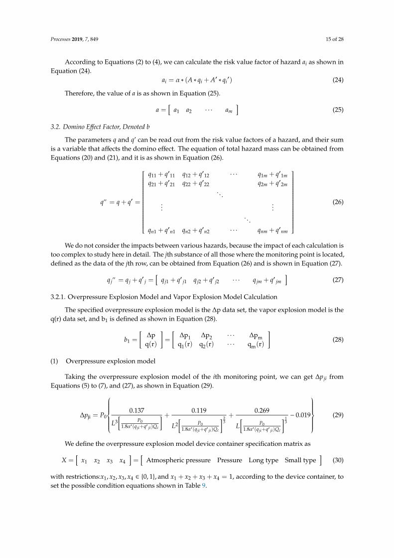
According to Equations (2) to (4), we can calculate the risk value factor of hazard ai as shown inEquation (24).

ai = α ∗ (A ∗ qi + A′ ∗ qi′) (24)

Therefore, the value of a is as shown in Equation (25).

a =[

a1 a2 · · · am]

(25)

3.2. Domino Effect Factor, Denoted b

The parameters q and q’ can be read out from the risk value factors of a hazard, and their sumis a variable that affects the domino effect. The equation of total hazard mass can be obtained fromEquations (20) and (21), and it is as shown in Equation (26).

q′′ = q + q′ =

q11 + q′11 q12 + q′12 · · · q1m + q′1mq21 + q′21 q22 + q′22 q2m + q′2m

. . ....

.... . .

qn1 + q′n1 qn2 + q′n2 · · · qnm + q′nm

(26)

We do not consider the impacts between various hazards, because the impact of each calculation istoo complex to study here in detail. The jth substance of all those where the monitoring point is located,defined as the data of the jth row, can be obtained from Equation (26) and is shown in Equation (27).

q j′′ = q j + q′ j =

[q j1 + q′ j1 q j2 + q′ j2 · · · q jm + q′ jm

](27)

3.2.1. Overpressure Explosion Model and Vapor Explosion Model Calculation

The specified overpressure explosion model is the ∆p data set, the vapor explosion model is theq(r) data set, and b1 is defined as shown in Equation (28).

b1 =

[∆p

q(r)

]=

[∆p1 ∆p2 · · · ∆pm

q1(r) q2(r) · · · qm(r)

](28)

(1) Overpressure explosion model

Taking the overpressure explosion model of the ith monitoring point, we can get ∆p ji fromEquations (5) to (7), and (27), as shown in Equation (29).

∆pji = P0

0.137

L3[

P01.8α′(q ji+q′ ji)Qc

] + 0.119

L2[

P01.8α′(q ji+q′ ji)Qc

] 23

+0.269

L[

P01.8α′(q ji+q′ ji)Qc

] 13

− 0.019

(29)

We define the overpressure explosion model device container specification matrix as

X =[

x1 x2 x3 x4]=

[Atmospheric pressure Pressure Long type Small type

](30)

with restrictions:x1, x2, x3, x4 ∈ {0, 1}, and x1 + x2 + x3 + x4 = 1, according to the device container, toset the possible condition equations shown in Table 9.

Processes 2019, 7, 849 16 of 28

Table 9. Overpressure model equipment container condition correspondence table.

Number x Value Condition Result

1 x1 = 1 ∆p ≥ 22 kpa b2 = Y=−18.96 + 2.44lnPs∆p < 22 kpa b3 = 0

2 x2 = 1 ∆p ≥ 16 kpa b2 = Y=−42.44 + 4.33lnPs∆p < 16 kpa b3 = 0

3 x3 = 1 ∆p ≥ 31 kpa b2 = Y=−28.07 + 3.16lnPs∆p < 31 kpa b3 = 0

4 x4= 1 ∆p ≥ 37 kpa b2 = Y=−17.79 + 2.18lnPs∆p < 37 kpa b3 = 0

(2) Vapor explosion modell

Taking the vapor explosion model of the ith monitoring point, we can get qji(r) and ti fromEquations (8) to (10), and (27), as shown in Equations (31) and (32).

qji(r) =q0

[2.9 ∗

(q ji + q′ ji

)1/3]2

r(1− 0.058lnr){[2.9 ∗

(q ji + q′ ji

)1/3]2+ r2

}3/2(31)

tji = 0.45 ∗(q ji + q′ ji

)1/3(32)

We define the vapor explosion model device container specification matrix as shown inEquation (33).

Y =[

y1 y2]=

[Atmospheric pressure Pressure

](33)

With restrictions y1, y2 ∈ {0, 1}, and y1 + y2 = 1, according to the device container, to set thepossible condition equations in Table 10.

Table 10. Steam model equipment container condition correspondence table.

Number y Value Condition Result

1 y1 = 1 qji(r) ≥ 15 kpa and t ≥ 10 min b2 = Y = 12.54 − 1.847(−1.128lnI − 2.667 × 10−5V + 9.877)qji(r) < 15 kpa or t < 10 min b3 = 0

2 y2 = 1 qji(r) ≥ 50 kpa and t ≥ 10 min b2 = Y = 12.54−1.847(−0.947lnI + 8.835V0.032)qji(r) < 50 kpa or t < 10 min b3 = 0

3.2.2. Overpressure Explosion and Vapor Explosion Model Probability Calculations

We define the overpressure explosion probability as the b3i data set and the vapor explosionprobability as the b’3i data set; the explosion probability matrix can then be constructed as shown inEquations (34) to (36).

b3 =

[b31 b32 · · · b3m

b′31 b′32 · · · b′3m

](34)

b3i =1√

2π

∫ b2i−5

−∞

e−x2/2dx (35)

b′3i =1√

2π

∫ b′2i−5

−∞

e−x2/2dx (36)

Processes 2019, 7, 849 17 of 28

3.2.3. Domino Effect Coefficient

Because the multilayer domino effect is complicated, but the calculation method is the same,we only consider the domino effect for a single layer. According to Equation (12), the domino effectcoefficient is as shown in Equation (37).

b4i = (1 + b3i)(1 + b′3i) (37)

The output domino effect coefficient b is as shown in Equation (38).

b =[

b41 b42 · · · b4m]

(38)

3.3. Operator Factor, Denoted c

In the calculation of the operator’s index coefficient, there are five items involved in the calculationof important information: the post (g), certificate (t1), working age (t2), accident-free time (t3), andworking time (t4).We set the input matrix as shown in Equation (39).

Ci =

Name 1Name 2

...

Name n

=

g1 t11 t21 t31 t41

g2 t12 t22 t32 t42

......

......

...

gn t1n t2n t3n t4n

i

(39)

This article uses real-time quantitative data, so there is no situation of different people in the samelocation; that is, N = 1 and M0 = N0.When gk = gj (k , j, k = 1,2, . . . ,n, j = 1,2, . . . ,n), from Equations(13)–(15), Hpi is as shown in Equation (40).

Hpi =n∏

j=1

1− 1

k2( t2

T2+ 1

) ∗1− 1

k3

(( t3T3

)2+ 1

) ∗

1− k4

(t4

T4− 1

)2 (40)

The elements u in the set {g1,g2, . . . ,gn}i can make up Hp, so the operator risk is as shown inEquation (41).

Hui = 1−mΠj=1

(1−Hpj

)(41)

From the calculation process, it can be seen that Hu has a maximum close to 1. Taking intoaccount the limited impact of personnel factors, when the value is 0.8, the coefficient c is specified as 1.The worse the indicator, the greater the coefficient c. The highest value of Hu is 1 and the lowest valueis specified as 0.6, so when the value is lower than 0.6, it is calculated using 0.6 instead. Therefore, therange of c values is 0.8 to 1.33.

When Hui ≤ 0.6, we let Hui = 0.6, and ci is calculated as shown in Equation (42).

ci =0.8Hui

(42)

The coefficient c is as shown in Equation (43).

c =[

c1 c2 · · · cm]

(43)

Processes 2019, 7, 849 18 of 28

3.4. Process/Equipment Factor, Denoted d

The process/equipment index factor includes a total of 13 second-level factors, namely, equipmentmaintenance, explosion-proof devices, inert gas protection, emergency cooling, emergency powersupply, electrical explosion-proofing, anti-static, lightning protection, devices for preventing fire,process parameter control, leak detection device and response, fault alarm and control devices, andaccidental discharge and treatment. There is a certain number of third-level index factors for eachsecond-level index factor, and the scores for each third-level index factor are not the same. There aretwo kinds of calculation logic, “and” and “or”, for the third-level indices, with the highest total scorebeing 310 points. Coefficient d is defined as 1 at 248 points (80%), and the worse the indicator, thegreater the coefficient d. The highest is 310 points, and when the value is less than 186 points (60%),it is calculated using 186 points. Therefore, the range of d values is 0.8 to 1.33.

According to Table 5, the score matrix

D = [8 6 24 11 13 15 10 12 12 7 7 7 12 11 11 15 11 11 10 13 10 11 13 13 14 11]

can be built for input data Xi, where

Xi = [X11 X12 X21 X22 X31 X32 X41 X42 X5 X6 X7 X8 X9 XA XB1 XB2 XC1 XC2 XC3 XC4 XC5 XD1 XD2 XD3 XD4 XD5]T

with restrictions as follows:

(1) The original input data are only 0 or 1, that is, X11, X12, . . . , XD5 ∈ {0,1};(2) X11 + X12 ≤ 1;(3) X31 + X32 ≤ 1;(4) X41 + X42 ≤ 1;(5) X5 = X51 + X52 ≤ 1;(6) X6 = X61 + X62 + X63 + X64 + X65 + X66 + X67 + X68 + X69 ≤ 1;(7) X7 = X71 + X72 + X73 + X74 + X75 ≤ 1;(8) X8 = X81 + X82 + X83 + X84 + X85;(9) X9 = X91 + X92 + X93;(10) XA = XA1 + XA2 + XA3 ≤ 1;(11) XB1 + XB2 ≤ 1.

According to the above score matrix, input data, and restrictions, we can get xi, where xi is themultiplication of matrix D and matrix Xi, as shown in Equation (44).

xi = DXi (44)

when xi ≥ 186, the definition of value d is as shown in Equation (45).

di =248xi

(45)

when xi < 186, the definition of value d is di = 1.33.The process/equipment index coefficient d is as shown in Equation (46).

d =[

d1 d2 · · · dm]

(46)

3.5. Building Environmental Factor, Denoted e

The building environmental index factor includes a total of five second-level factors, namely,ventilation plant, pressure relief, monitoring device, plant structure, and industrial sewer. There area certain number of third-level index factors for each second-level index factor, and the third-level

Processes 2019, 7, 849 19 of 28

index factor scores are not the same. There are two kinds of calculation logic, “and” and “or”, for thethird-level indices, with the highest total score being 89 points. Coefficient e is defined as 1at 71 points(80%), and the worse the indicator, the greater the coefficient e. The highest is 89 points, and when thevalue is less than 53 points (60%), it is calculated using 53 points. Therefore, the range of e values is 0.8to 1.33.

According to Table 4, the score matrix

E = [6 8 8 8 10 12 18 5 5 5 5 5 5 5]

can be built with input data Yi such that Yi= [Y11 Y21 Y22 Y23 Y31 Y32 Y33 Y41 Y42 Y43 Y44 Y45 Y51 Y52]T

and with restrictions as follows:

(1) The original input data are only 0 or 1, that is, Y11, Y21, . . . , Y52 ∈ {0,1};(2) Y21 + Y22 + Y23 ≤ 1.

According to the above score matrix, input data, and restrictions, we can get yi where yi is themultiplication of matrix E and matrix Yi, as shown in Equation (47).

yi = EYi (47)

when yi ≥ 53, the definition of e is as shown in Equation (48).

ei =71yi

(48)

when yi < 53, the definition of e is ei = 1.33.The construction environmental index coefficient e is as shown in Equation (49).

e =[

e1 e2 · · · em]

(49)

3.6. Safety Management Factor, Denoted f

The safety management index factor includes a total of 10 s-level factors, namely, safety productionresponsibility system, safety education, safety technical measures plan, safety inspection, safety rulesand regulations, safety management agencies and personnel, statistical analysis of accidents, hazardassessment and rectification, contingency plans and measures, and fire safety management. There are acertain number of third-level index factors for each second-level index factor, and the third-level indexfactor scores are not the same. The total score is 100 points. At 80 points, coefficient f is defined as 1,and the worse the indicator, the greater the coefficient f. The highest is 100 points, and when the valueis less than 60 points, it is calculated using 60 points. Therefore, the range of f values is 0.8 to 1.33.

According to Table 5, score matrix

F = [1.1 1.25 2.50 1.43 0.77 2.00 3.30 2.50 1.11 1.00]

can be built for input data Zi, where Zi= [Z1 Z2 Z3 Z4 Z5 Z6 Z7 Z8 Z9 ZA]T, with restrictions as follows:

(1) The original input data are only 0 or 1, that is, Z11, Z12, . . . , ZAA ∈ {0,1};(2) Z1 = Z11 + Z12 + Z13 + Z14 + Z15 + Z16 + Z17 + Z18 + Z19;(3) Z2 = Z21 + Z22 + Z23 + Z24 + Z25 + Z26 + Z27 + Z28;(4) Z3 = Z31 + Z32 + Z33 + Z34;(5) Z4 = Z41 + Z42 + Z43 + Z44 + Z45 + Z46 + Z47;(6) Z5 = Z51 + Z52 + Z53 + Z54 + Z55 + Z56 + Z57 + Z58 + Z59 + Z5A + Z5B + Z5C + Z5D;(7) Z6 = Z61 + Z62 + Z63 + Z64 + Z65;(8) Z7 = Z71 + Z72 + Z73;

Processes 2019, 7, 849 20 of 28

(9) Z8 = Z81 + Z82 + Z83 + Z84 + Z85 + Z86 + Z87 + Z88 + Z89;(10) Z9 = Z91 + Z92 + Z93 + Z94 + Z95 + Z96 + Z97 + Z98 + Z99;(11) ZA = ZA1 + ZA2 + ZA3 + ZA4 + ZA5 + ZA6 + ZA7 + ZA8 + ZA9 + ZAA.

According to the above score matrix, input data, and restrictions, we can get zi, where zi is themultiplication of matrix F and matrix Zi as shown in Equation (50).

zi = FZi (50)

when zi ≥ 60, the definition of f is as shown in Equation (51).

fi =80zi

(51)

when zi < 60, the definition of f is fi = 1.33.The safety management index coefficient f is as shown in Equation (52).

f =[

f1 f2 · · · fm]

(52)

3.7. Calculation Results

We used forced pair comparison (Table 11) to calculate the final optimized risk value R’ of thehazards. R’ is as shown in Equation (53):

Ri′ = R3i ∗

5∑j = 1

ωjKi(j) (53)

where Ki(j) is a five-point indicator function of i monitoring points.

Table 11. Pairwise comparison to determine the weight of each factor.

Evaluation Items One-to-One Comparison Result Points Accumulated Weight (ωj)

Domino effect 1 1 1 1 4 0.4

Operator 0 1 1 0 2 0.2

Process/equipment 0 0 1 0 1 0.1

Building environment 0 0 0 1 1 0.1

Safety management 0 1 1 0 2 0.2

Total 10 1.0

4. Case Analysis

4.1. Major Hazards Factory Fact Sheet

At present, there are a total of 64 chemical plants in the particular chemical industry park weare studying; each chemical plant in it has its own characteristics. This chemical industrial park ispotentially high-risk, and the chemical plants in the park are concentrated, and there are many majorhazards such as inflammable, explosive and toxic. Applying our dynamic semi-quantitative model,chemical park managers can understand and grasp the risk values and risk trends of each chemicalplant in the park, and further grasp the risk level of each chemical plant. For these chemical plantswhere the first-level risk or risk trend is bad, the chemical park managers should focus on monitoringand management, and notify the corresponding chemical plant to improve so as to reduce risks. One ofthe chemical plants is a high-yield one in this chemical industrial park, and a co-author of this articleis an employee of the chemical plant who was able to provide accurate data for calculations, so this

Processes 2019, 7, 849 21 of 28

chemical plant was chosen as a calculation case. The chemical plant has a spherical tank area whichhas two spherical tanks that are pressure vessels filled with methanol and ethanol, respectively. Thehazard masses are subject to real-time monitoring. We chose 15 monitoring points, that is, m=15, in themonitoring data and calculated the variable q in storage and the variable q’ in the production pipelineas follows (unit: ton). In the two rows of the matrices in the follow-up case, the one above is methanoland that below is ethanol, as shown in Equations (54) to (56).

q ∼ q′ ∼[

MethanolEthanol

](54)

The variables q and q’ were therefore calculated as shown in Equations (55) and (56).

q =

[200 70 80 180 250 200 150 350 180 120 210 300 50 80 260200 130 40 120 250 400 150 150 220 180 210 500 150 150 240

](55)

q′ =[

3 6 4 6 0 0 8 5 7 8 10 14 10 8 47 6 8 6 10 20 12 10 8 10 9 16 30 12 15

](56)

The resident population within 500 m of the hazards is 302, and the distance to a surroundinghazard is 70 m (the distance to other hazards is over 500 m, giving no possible impact). The names,post, certificate, working age, accident-free time, and working time of operators on the 15 monitoringpoints are shown in Table 12.

Table 12. Information on operators at the monitoring points.

MonitoringPoint Name Post Certificate Working

Age (Years)Accident-FreeTime (Years)

Working Time(Hours/Day)

1 Tom Storage Yes 1 1 82 Tom Storage Yes 1 1 93 Tom Storage Yes 1 1 104 Tom Storage Yes 1 1 85 Tom Storage Yes 2 2 86 Tom Storage Yes 2 0 87 Tom Storage Yes 2 0 108 Tom Storage Yes 2 1 89 Jack Storage Yes 5 5 8

10 Jack Storage Yes 5 5 1011 Mark Storage Yes 2 0 812 Mark Storage Yes 2 0 813 Mark Storage Yes 2 0 814 Jose Storage Yes 1 1 815 Joe Storage Yes 4 4 10

4.2. Dynamic Quantitative Calculation of Hazards

4.2.1. Risk Value Factor of Hazards, Denoted a

As the hazards are methanol and ethanol, we can look up the table to obtain α = 2; the resultingA and A′ are shown in Equation (57).

A =[

1.520

1.520

]and A′ =

[1.52

1.52

](57)

The value of a can be obtained from ai = α ∗ (A ∗ qi + A′ ∗ qi′) and a =

[a1 a2 · · · am

], as

shown in Equation (58).

a =[

75 48 36 63 90 120 75 97.5 82.5 72 91.5 165 90 64.5 103.5]

(58)

Processes 2019, 7, 849 22 of 28

4.2.2. Domino Effect Factor, Denoted b

From the risk value factor of hazards (previous section), we know that the parameters q and q’ arelarge variables that affect the domino effect. The total hazards calculation can then be obtained fromEquations (26) and (27), as shown in Equation (59) (unit: ton).

q′′ =[

203 76 84 186 250 200 158 355 187 128 220 314 60 88 264207 136 48 126 260 420 162 160 228 190 219 516 180 162 255

](59)

(1) Overpressure explosion

From the look-up table, α’ = 0.04, methanol’s heat of combustion Qc = 22,675 kJ/kg, ethanol’sheat of combustion Qc = 29,640 kJ/kg, p0 = 101,325 pa, and L = 70 m is given in the example; fromEquation (29), ∆p can be obtained as shown in Equation (60).

∆p =

[243 118 126 227 285 240 200 378 228 171 258 342 100 130 298304 219 103 207 365 542 251 248 328 284 318 645 272 251 359

](60)

Since it is a pressure vessel, b2 can be obtained according to Equation (30) and Table 9, and it is asshown in Equation (61).

b2 =

[11.2 8.1 8.4 11.0 12.0 11.2 10.4 13.2 11.0 9.7 11.5 12.7 7.4 8.6 12.112.2 10.8 7.5 10.6 13.0 14.7 11.4 11.3 12.6 11.9 12.4 15.5 11.7 11.4 12.9

](61)

Therefore, according to Equation (35), the probability of overpressure explosion is as shown inEquation (62).

b3c =

[1 1 1 1 1 1 1 1 1 1 1 1 1 1 11 1 1 1 1 1 1 1 1 1 1 1 1 1 1

](62)

(2) Vapor explosion

From the look-up table, q0 = 200 kw/m2, and L = 70 m is given in the example, so q(r) and t can beobtained from Equations (31) and(32) as shown in Equations(63) and (64).

q(r) =[

49 56 56 49 47 49 51 43 49 53 48 45 57 56 4649 53 58 53 47 42 51 51 48 50 48 40 50 51 47

](63)

t =[

26 19 20 26 28 26 24 32 26 23 27 31 18 20 2927 23 16 23 29 34 25 25 27 26 27 36 25 25 29

](64)

Since it is a pressure vessel, we claim q(r) ≥ 50 kpa and t ≥ 600 s (10 min). It can be seen fromthe above equation that t is less than 600 s, so they do not all produce the domino effect of a vaporexplosion; thus, the probability of vapor explosion is 0, as shown in Equation (65).

b′3c =

[0 0 0 0 0 0 0 0 0 0 0 0 0 0 00 0 0 0 0 0 0 0 0 0 0 0 0 0 0

](65)

(3) Domino effect coefficient

Methanol and ethanol produce the same domino effect, so we only need to take one set of data;from Equation (38), the domino effect coefficient b is as shown in Equation (66).

b =[

2 2 2 2 2 2 2 2 2 2 2 2 2 2 2]

(66)

Processes 2019, 7, 849 23 of 28

4.2.3. Operator Factor, Denoted c

From the input monitoring point operator post information in Table 12 and Equation (40), Hp canbe obtained as shown in Equation (67).

Hp =[

0.83 0.81 0.77 0.83 0.92 0.48 0.45 0.86 0.97 0.91 0.48 0.48 0.48 0.83 0.90]

(67)

According to Hp and Equation (41), Hu can be obtained as shown in Equation (68).

Hu =[

0.83 0.81 0.77 0.83 0.92 0.48 0.45 0.86 0.97 0.91 0.48 0.48 0.48 0.83 0.90]

(68)

when Hui ≤ 0.6, we let Hui = 0.6; the H’u values obtained after adjustment are as shown in Equation(69).

H′u =[

0.83 0.81 0.77 0.83 0.92 0.60 0.86 0.97 0.91 0.60 0.60 0.60 0.60 0.83 0.90]

(69)

By Equation (42), the available operator factor coefficient c is as shown in Equation (70).

c =[

0.97 0.99 1.03 0.97 0.87 1.33 1.33 0.94 0.82 0.88 1.33 1.33 1.33 0.97 0.88]

(70)

4.2.4. Process/Equipment Factor, Denoted d

From the input data Xi, a preliminary summary of available data is given in Table 13.

Table 13. Summary of input information for calculation of the process/equipment index.

XiMonitoring Points

1 2 3 4 5 6 7 8 9 10 11 12 13 14 15

X11 1 0 1 0 1 1 0 0 1 1 0 0 0 0 0X12 0 0 0 1 0 0 1 1 0 0 0 0 1 1 1X21 1 1 0 0 1 1 1 0 0 1 0 1 0 1 1X22 1 1 0 1 1 1 1 0 0 1 1 0 1 0 1X31 1 0 0 1 0 1 1 0 0 0 0 1 0 1 0X32 0 1 1 0 1 0 0 0 1 0 0 0 1 0 1X41 1 0 0 1 1 1 0 0 0 0 1 0 1 1 1X42 0 1 0 0 0 0 0 0 1 1 0 0 0 0 0X5 1 0 0 1 1 1 1 1 1 1 0 0 1 1 1X6 1 0 1 1 1 0 1 0 1 0 1 1 1 0 0X7 1 0 0 1 1 1 0 0 1 1 0 0 1 1 1X8 2 3 5 4 1 3 4 5 2 3 5 5 2 4 3X9 3 2 1 1 2 2 2 2 3 3 3 2 2 1 1XA 1 0 1 1 1 0 0 1 1 1 1 0 0 0 0XB1 1 1 0 0 0 0 1 1 1 1 0 1 0 1 1XB2 0 0 1 1 1 0 0 0 0 0 1 0 0 0 0XC1 1 1 1 0 1 1 1 1 1 1 1 1 0 1 0XC2 0 1 1 1 0 1 1 1 1 0 1 0 0 0 0XC3 0 1 1 1 0 0 1 1 1 1 1 1 0 0 0XC4 1 1 1 1 0 0 0 1 0 0 0 1 1 0 1XC5 1 1 1 1 1 1 0 0 0 0 0 1 1 0 1XD1 1 1 1 1 1 1 0 0 0 0 0 1 1 0 1XD2 1 1 1 0 1 1 1 0 1 0 1 1 1 0 1XD3 0 1 1 0 1 1 1 0 0 1 1 1 1 0 1XD4 0 1 1 0 0 0 1 1 1 1 1 1 1 0 1XD5 1 1 0 0 1 0 0 1 0 1 1 1 0 0 1

From xi=DXi, xi can be obtained as shown in Equation (71).

x =[

278 235 209 187 220 199 208 169 192 212 208 220 180 134 214]

(71)

Processes 2019, 7, 849 24 of 28

According to the value of x, we can further calculate d as shown in Equation (72).

d =[

0.89 1.06 1.19 1.33 1.13 1.25 1.19 1.33 1.29 1.17 1.19 1.13 1.33 1.33 1.16]

(72)

4.2.5. Building Environmental Factor, Denoted e

From the input data Yi, a preliminary summary of available data is given in Table 14.

Table 14. Summary of input information for calculation of the building environmental index.

YiMonitoring Points

1 2 3 4 5 6 7 8 9 10 11 12 13 14 15

Y11 1 0 1 0 1 1 0 1 1 1 0 0 0 0 1Y21 1 0 0 0 0 0 1 0 0 1 0 1 0 1 1Y22 0 1 0 1 1 1 0 0 0 0 1 0 1 0 0Y23 0 0 0 0 0 0 0 1 1 0 0 0 0 0 1Y31 1 1 0 1 0 1 1 1 1 0 1 1 0 1 0Y32 1 1 1 0 1 0 1 0 1 0 0 0 1 0 1Y33 1 1 1 1 0 1 0 1 1 1 1 1 1 1 1Y41 1 0 0 1 1 1 0 0 0 0 1 0 1 1 1Y42 0 1 0 0 0 0 0 0 1 1 0 1 0 0 0Y43 1 0 0 1 1 1 1 1 1 1 0 0 1 1 1Y44 1 0 1 1 1 0 1 0 1 0 1 1 1 0 0Y45 1 0 0 1 1 1 0 1 1 1 1 0 1 1 1Y51 1 1 1 0 0 0 1 1 1 1 1 0 0 1 1Y52 1 1 1 1 0 0 0 1 1 0 1 0 1 1 1

From yi = DYi, we can calculate y, and it is as shown in Equation (73).

y =[

84 63 51 61 46 57 45 62 84 52 61 46 63 61 77]

(73)

According to the value of y, we can further calculate e as shown in Equation (74).

e =[

0.85 1.13 1.33 1.16 1.33 1.25 1.33 1.15 0.85 1.33 1.16 1.33 1.13 1.16 0.92]

(74)

4.2.6. Safety Management Factor, Denoted f

From the input data Zi, a preliminary summary of available data is given in Table 15.

Table 15. Summary of input information for calculation of the safety management index.

ZiMonitoring Points

1 2 3 4 5 6 7 8 9 10 11 12 13 14 15

Z1 10 10 10 7.7 6.6 10 3 10 8.8 7.7 10 8.8 7.7 10 10Z2 10 8.8 8.8 7.5 7.5 8.8 8.8 7.5 7.5 10 10 10 7.5 7.5 10Z3 10 7.5 7.5 5.0 5.0 5.0 7.5 10 10 10 7.5 7.5 10 10 7.5Z4 10 8.6 8.6 7.1 7.1 5.7 7.1 7.1 8.6 8.6 8.6 10 10 10 8.6Z5 10 9.2 9.2 8.5 8.5 6.9 6.9 10 10 10 6.9 6.9 8.5 9.2 10Z6 10 8.0 10 10 8.0 6.0 8.0 6.0 10 10 10 6.0 6.0 10 8.0Z7 10 10 6.6 6.6 6.6 6.6 3.3 10 10 10 10 6.6 6.6 10 10Z8 10 10 7.5 5.0 5.0 5.0 2.5 7.5 7.5 7.5 10 10 10 10 10Z9 10 10 10 6.6 7.7 8.8 5.5 10 10 8.8 7.7 7.7 8.8 6.6 10ZA 8 9.0 9.0 10 8.0 9.0 5.0 9.0 9.0 7.0 7.0 8.0 10 10 9.0

From zi = FZi, we can calculate z as shown in Equation (75).

z =[

98 91 87 74 70 72 58 87 91 90 88 82 85 93 93]

(75)

Processes 2019, 7, 849 25 of 28

According to the value of z, we can further calculate f as shown in Equation (76).

f =[

0.82 0.88 0.92 1.08 1.14 1.11 1.33 0.92 0.88 0.89 0.91 0.98 0.94 0.86 0.86]

(76)

4.3. The Final Optimized Hazard Risk Value

According to Equation (53), we can get R’; the specific values of R’ are shown in Equation (77),and the data trend of R’ is shown in Figure 4.

R′ =[

99.9 66.9 51.9 91.9 130.2 184.6 118.8 138.5 111.7 101.1 135.7 248.8 135.0 91.3 140.4]

(77)

Figure 4. Evaluation results trend.

4.4. Comparison WITH the Traditional Method of Calculating Hazard Risk Values

The traditional R value can be calculated using Equation (1), as shown in Equation (78).

R =[

60 30 18 45 75 90 45 75 60 45 63 120 30 34.5 75]

(78)

The risk value comparison results are shown in Figure 5. According to the data in Figure 5, thetraditional R value only considers the hazard of the storage area in the chemical plant, and the riskvalue is thus relatively low. Only one point out of the 15 monitored time points exceeds the first levelof the danger standard value of 100. The final optimized hazard risk value was calculated from datafrom hazards in the storage area, hazards in the processing pipelines, the domino effect, operators,process/equipment, the building environment, and safety management. Out of the 15 monitoringpoints in time, 10 points exceeded the first level of the danger standard value of 100, and it is obviousthat the optimized risk value has a more realistic result. Using the optimized hazard risk value as anindicator of the overall risk assessment in chemical plants, the real-time data of the six influencingfactors can be obtained separately, which can greatly help in the safety analysis of chemical plants.For example, when R’ ≥ 100, the chemical plant is a first-level risk and needs to be heavily regulated.The chemical industry park managers can monitor the risk value fluctuations of these first-level riskchemical plants in real time. At the same time, the data can be used to determine which one of thesix factors is the most influential on the danger risk value; this can then be used to find the source ofthe problem in time and arrange immediate improvements to reduce the chemical plant risk level tosecondary risk. If it cannot be reduced to secondary risk, other measures need to be provided to ensurethe safety of chemical production and to prevent accidents. Attention must be paid to trends in therisk value in real time. Once there is an abnormality, it is necessary to stop production and handle theabnormality in time. Here, the threshold (R = 100) is a criterion in the calculation of the traditionalrisk value. As the six factors increase, the threshold will change. This optimized threshold for R’ also

Processes 2019, 7, 849 26 of 28

needs to be accurate after statistics and calculations based on long-term data; in subsequent use, thethreshold will be formulated according to the actual situation.

Figure 5. The final optimized risk value trend in contrast with the traditional risk value trend.

5. Conclusions

In this article, we proposed and analyzed a new dynamic semi-quantitative risk calculation modelfor chemical plants that can be applied digitally. This model provides a sustainable, standardized,and comprehensive management strategy for the safety management of chemical plants and chemicalindustry park managers. The model and its determined parameters were applied to the dynamicsemi-quantified safety management of chemical plants with in the chemical industry park of Quzhou,Zhejiang Province. From the point of view of the existing semi-quantitative model, the existingproblems of the current model were analyzed, the current model was optimized, and a new dynamicsemi-quantitative evaluation model scheme was proposed. The new model employs an analyticalhierarchy process to comprehensively assess and compare the differences in the risk values of hazardsamong plants. The dynamic semi-quantitative calculation system for managing hazards is composedof six elements: operator, process/equipment, hazard risk, building environment, safety management,and domino effect. The model finally produces a dynamic quantification value, which can be usedto compare the risk value of the chemical company from six angles directly reflected through thecorresponding software, allowing it to play a greater role in the safety management of the plant.The establishment of this model involves many basic disciplines, such as management, mathematics,operations research, control science, computer science, etc. A combination of these basic disciplineswas used to get this dynamic quantitative risk value. Of course, the model is not perfect, giving room tofurther optimize the threshold and some parameter settings in future to make the model more practicaland accurate. In addition to the above research topics, future research should also explore other aspectsof chemical safety management in order to establish a complete chemical safety management andemergency rescue system. At the same time, we will continue to study the systematic engineeringneeded to combine the many basic disciplines involved in the model and use the thinking of systemengineering to establish a theoretical framework of modern safety engineering based on safety riskanalysis management.

Author Contributions: Q.S. and P.J. proposed the computational model and wrote the paper. S.Z. and Y.K.contributed to the analysis of the results. Y.Z. and G.S. contributed to the data. All the authors reviewedthe manuscript.

Funding: This work was supported by the Provincial Key R&D Program of Zhejiang Province (No. 2017C03019),National Key R&D Program of China (No. 2016YFC0201400), International Science and Technology CooperationProgram of Zhejiang Province for Joint Research in High-tech Industry (No. 2016C54007), Zhejiang Joint Fund forIntegrating of Informatization and Industrialization (No. U1509217), and National Natural Science Foundation ofChina (No. U1609212).

Processes 2019, 7, 849 27 of 28

Conflicts of Interest: There are no conflicts to declare.

References

1. Willey, R.J.; Hendershot, D.C.; Berger, S. Berger The Accident in Bhopal: Observations 20 Years Later. ProcessSaf. Prog. 2010, 26, 180–184. [CrossRef]

2. Shallcross, D.C. Using concept maps to assess learning of safety case studies—The Piper Alpha disaster.Educ. Chem. Eng. 2013, 8, e1–e11. [CrossRef]

3. Tauseef, S.M.; Abbasiand, T.; Abbasi, S.A. Development of a new chemical process-industry accident databaseto assist in past accident analysis. J. Loss Prev. Process Ind. 2011, 24, 426–431. [CrossRef]

4. Manca, D.; Brambilla, S. Dynamic simulation of the BP Texas City refinery accident. J. Loss Prev. Process Ind.2012, 25, 950–957. [CrossRef]

5. Pittman, W.; Han, Z.; Harding, B.; Rosas, C.; Jiang, J.; Pineda, A.; Mannan, M.S. Lessons to be learned from ananalysis of ammonium nitrate disasters in the last 100 years. J. Hazard. Mater. 2014, 280, 472–477. [CrossRef][PubMed]

6. Jain, P.; Rogers, W.J.; Pasman, H.J.; Keim, K.K.; Mannan, M.S. A Resilience-Based Integrated Process SystemsHazard Analysis (RIPSHA) Approach: Part I Plant System Layer. Process Saf. Environ. Prot. 2018, 116, 92–105.[CrossRef]

7. Bottelberghs, P.H. Risk analysis and safety policy developments in the Netherlands. J. Hazard. Mater. 2000,71, 59. [CrossRef]

8. Zarei, E.; Azadeh, A.; Khakzad, N.; Aliabadi, M.M.; Mohammadfam, I. Dynamic safety assessment of naturalgas stations using Bayesian network. J. Hazard. Mater. 2017, 321, 830–840. [CrossRef] [PubMed]

9. Cahen, B. Implementation of new legislative measures on industrial risks prevention and control in urbanareas. J. Hazard. Mater. 2006, 130, 293–299. [CrossRef] [PubMed]

10. Khan, F.I.; Amyotte, P.R. I2SI: A comprehensive quantitative tool for inherent safety and cost evaluation.J. Loss Prev. Process Ind. 2005, 18, 310–326. [CrossRef]

11. Khakzad, N.; Khanand, F.; Amyotte, P. Quantitative risk analysis of offshore drilling operations: A Bayesianapproach. Saf. Sci. 2013, 57, 108–117. [CrossRef]

12. Abimbola, M.; Khan, F.; Khakzad, N.; Butt, S. Safety and risk analysis of managed pressure drilling operationusing Bayesian network. Saf. Sci. 2015, 76, 133–144. [CrossRef]

13. Goerlandt, F.; Khakzadand, N.; Reniers, G. Validity and validation of safety-related quantitative risk analysis:A review. Saf. Sci. 2016, 99, 127–139. [CrossRef]

14. De, D.V.; Fiévez, C. ARAMIS project: A more explicit demonstration of risk control through the use ofbow-tie diagrams and the evaluation of safety barrier performance. J. Hazard. Mater. 2006, 130, 220–233.

15. Delvosalle, C.; Fievez, C.; Pipart, A.; Debray, B. ARAMIS project: A comprehensive methodology for theidentification of reference accident scenarios in process industries. J. Hazard. Mater. 2006, 130, 200. [CrossRef][PubMed]

16. Abdolhamidzadeh, B.; Abbasi, T.; Rashtchian, D.; Abbasi, S.A. A new method for assessing domino effect inchemical process industry. J. Hazard. Mater. 2010, 184, 416. [CrossRef] [PubMed]

17. Jonkman, S.N.; Van Gelder, P.H.A.J.M.; Vrijling, J.K. An overview of quantitative risk measures for loss of lifeand economic damage. J. Hazard. Mater. 2003, 99, 1–30. [CrossRef]

18. Arendt, J.S. Using quantitative risk assessment in the chemical process industry. Reliab. Eng. Syst. Saf. 1990,29, 133–149. [CrossRef]

19. Khan, F.I.; Abbasi, S.A. Techniques and methodologies for risk analysis in chemical process industries. J. LossPrev. Process Ind. 1998, 11, 261–277. [CrossRef]

20. Sciver, G.R.V. Quantitative risk analysis in the chemical process industry. Reliab. Eng. Syst. Saf. 1990, 29,55–68. [CrossRef]

21. Christou, M.D.; Mattarelli, M. Land-use planning in the vicinity of chemical sites: Risk-informed decisionmaking at a local community level. J. Hazard. Mater. 2000, 78, 191. [CrossRef]

22. Christou, M.D.; Amendolaand, A.; Smeder, M. The control of major accident hazards: The land-use planningissue. J. Hazard. Mater. 1999, 65, 151–178. [CrossRef]

23. Hauptmanns, U. A risk-based approach to land-use planning. J. Hazard. Mater. 2005, 125, 1–9. [CrossRef][PubMed]

Processes 2019, 7, 849 28 of 28

24. Dechy, N.; Mouilleau, Y. Some lessons of the Toulouse disaster, 21st september 2001. In Proceedings of theHRO International Conference 2007, Deauville, France, 29–31 May 2007.

25. Spaziante, A.; Carpignano, A. Land use planning around Seveso installations: The Italian approach.Res. Nurs. Health 2001, 8, 1763.

26. Basta, C.; Neuvel, J.M.; Zlatanova, S.; Ale, B. Risk-maps informing land-use planning processes A surveyon the Netherlands and the United Kingdom recent developments. J. Hazard. Mater. 2007, 145, 241–249.[CrossRef] [PubMed]

27. Cozzani, V.; Bandini, R.; Basta, C.; Christou, M.D. Application of land-use planning criteria for the control ofmajor accident hazards: A case-study. J. Hazard. Mater. 2006, 136, 170–180. [CrossRef] [PubMed]

28. Khakzad, N.; Reniers, G. Risk-based design of process plants with regard to domino effects and land useplanning. J. Hazard. Mater. 2015, 299, 289–297. [CrossRef] [PubMed]

29. Huang, L.; Wan, W.; Li, F.; Li, B.; Yang, J.; Bi, J. A two-scale system to identify environmental risk of chemicalindustry clusters. J. Hazard. Mater. 2011, 186, 247–255. [CrossRef] [PubMed]

30. Brown, D.F.; Dunn, W.E. Application of a quantitative risk assessment method to emergency responseplanning. Comput. Oper. Res. 2007, 34, 1243–1265. [CrossRef]

31. Planas, E.; Arnaldos, J.; Silvetti, B.; Vallée, A.; Casal, J. A risk severity index for industrial plants and sites.J. Hazard. Mater. 2006, 130, 242–250. [CrossRef] [PubMed]

32. Dakkoune, A.; Vernières-Hassimi, L.; Leveneur, S.; Lefebvre, D.; Estel, L. Risk analysis of French chemicalindustry. Saf. Sci. 2018, 105, 77–85. [CrossRef]

33. Leveson, N. A new accident model for engineering safer systems. Saf. Sci. 2004, 42, 237–270. [CrossRef]34. Leveson, N. A systems approach to risk management through leading safety indicators. Reliab. Eng. Syst. Saf.

2015, 136, 17–34. [CrossRef]35. Cozzani, V.; Gubinelli, G.; Antonioni, G.; Spadoni, G.; Zanelli, S. The assessment of risk caused by domino

effect in quantitative area risk analysis. J. Hazard. Mater. 2005, 127, 14–30. [CrossRef] [PubMed]36. Othman, M.R.; Idris, R.; Hassim, M.H.; Ibrahim, W.H.W. Prioritizing HAZOP analysis using analytic

hierarchy process (AHP). Clean Technol. Environ. Policy 2016, 18, 1345–1360. [CrossRef]37. Cozzani, V.; Gubinelliand, G.; Salzano, E. Escalation thresholds in the assessment of domino accidental

events. J. Hazard. Mater. 2006, 129, 1–21. [CrossRef] [PubMed]

© 2019 by the authors. Licensee MDPI, Basel, Switzerland. This article is an open accessarticle distributed under the terms and conditions of the Creative Commons Attribution(CC BY) license (http://creativecommons.org/licenses/by/4.0/).