1 07. The planning problem 2 Inputs: 1. A description of the world state 2. The goal state...

1

07

Alireza yousefpour [email protected]

2

The planning problem

Inputs:1. A description of the world state2. The goal state description3. A set of actions

Output:A sequence of actions that if applied to the

initial state, transfers the world to the goal state

3

An example – Blocks world

Blocks on a table Can be stacked, but only one block on top

of another A robot arm can pick up a block and move

to another position On the table On another block

Arm can pick up only one block at a time Cannot pick up a block that has another one

on it

4

STRIPS Representation

State is a conjunction of positive ground literals

On(B, Table) Λ Clear (A) Goal is a conjunction of positive ground

literals Clear(A) Λ On(A,B) Λ On(B, Table)

STRIPS Operators Conjunction of positive literals as preconditions Conjunction of positive and negative literals as

effects

5

More on action schema

Example: Move (b, x, y) Precondition:

Block(b) Λ Clear(b) Λ Clear(y) Λ On(b,x) Λ (b ≠ x) Λ (b ≠ y) Λ (y ≠ x)

Effect: ¬Clear(y) Λ ¬On(b,x) Λ Clear(x) Λ On(b,y)

An action is applicable in any state that satisfies its precondition

Delete list Add list

6

STRIPS assumptions

Closed World assumption Unmentioned literals are false (no need to

explicitly list out) STRIPS assumption

Every literal not mentioned in the “effect” of an action remains unchanged

Atomic Time (actions are instantaneous)

7

STRIPS expressiveness

Literals are function free: Move (Block(x), y, z)

operators can be propositionalized

Move(b,x,y) and 3 blocks and table can be expressed as 48 purely propositional actions

No disjunctive goals: On(B, Table) V On(B, C)

No conditional effects: On(B, Table) if ¬On(A, Table)

8

Planning algorithms

Planning algorithms are search procedures

Which state to search? State-space search

Each node is a state of the world Plan = path through the states

Plan-space search Each node is a set of partially-instantiated

operators and set of constraints Plan = node

9

State search

Search the space of situations, which is connected by operator instances

The sequence of operators instances = plan

We have both preconditions and effects available for each operator, so we can try different searches: Forward vs. Backward

10

Planning: Search Space

AC

B A B C A CB

CBA

BA

C

BAC

B CA

CAB

ACB

BCA

A BC

AB

C

ABC

11

Forward state-space search (1)

Progression Initial state: initial state of the problem Actions:

Applied to a state if all the preconditions are satisfied

Succesor state is built by updating current state with add and delete lists

Goal test: state satisfies the goal of the problem

12

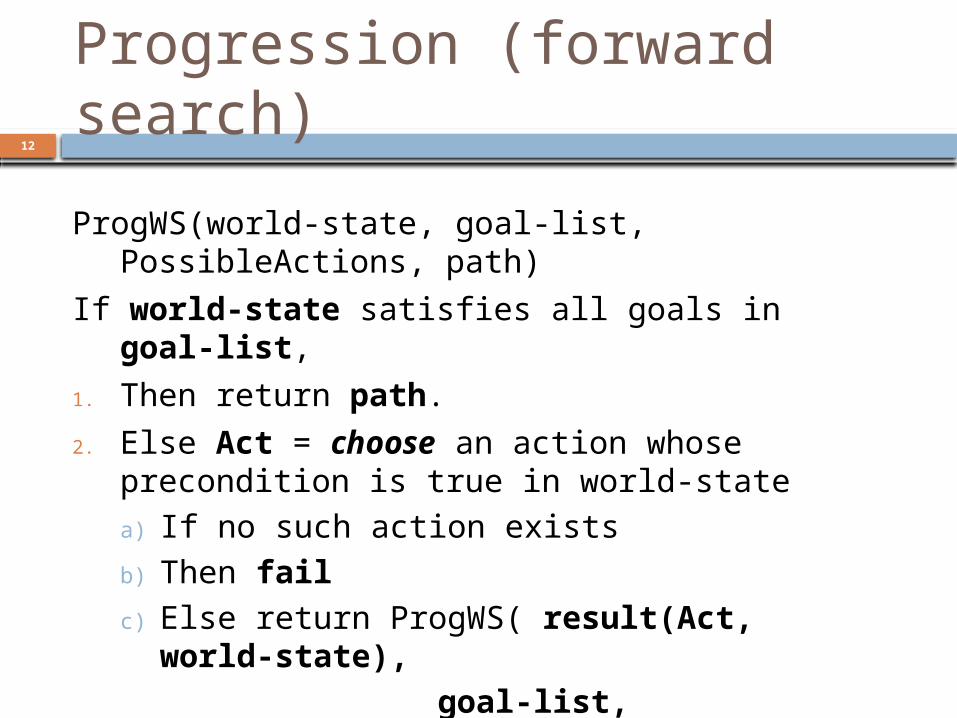
Progression (forward search)

ProgWS(world-state, goal-list, PossibleActions, path)

If world-state satisfies all goals in goal-list,

1. Then return path.

2. Else Act = choose an action whose precondition is true in world-statea) If no such action existsb) Then failc) Else return ProgWS( result(Act, world-

state), goal-list,

PossibleActions, concatenate(path,

Act) )

13

Forward search in the Blocks world

…

…

14

Forward state-space search (2)

Advantages No functions in the declarations of goals

search state is finite Sound Complete (if algorithm used to do the

search is complete) Limitations

Irrelevant actions not efficient Need heuristic or pruning procedure

15

Backward state-space search (1)

Regression Initial state: goal state of the problem Actions:

Choose an action that Is relevant; has one of the goal literals in its effect

set Is consistent; does not negate another literal

Construct new search state Remove all positive effects of A that appear in goal Add all preconditions, unless already appears

Goal test: state is the initial world state

16

Regression (backward search)RegWS(initial-state, current-goals, PossibleActions,

path)1. If initial-state satisfies all of current-goals2. Then return path3. Else Act = choose an action whose effect

matches one of current-goalsa. If no such action exists, or the effects of Act

contradict some of current-goals, then failb. G = (current-goals – goals-added-

by(Act)) + preconds(Act)c. If G contains all of current-goals, then faild. Return RegWS(initial-state, G,

PossibleActions, concatenate(Act,

path))

17

Backward state-space search (2)

Advantages Consider only relevant actions much

smaller branching factor Limitations

Still need heuristic to be more efficient

18

Comparing ProgWS and RegWS

Both algorithms are sound (they always return a valid plan) complete (if a valid plan exists they will find

one)

Running time is O(bn)where b = branching factor,

n = number of “choose” operators

19

Blocks world: STRIPS operators

Pickup(x)Pre: on(x, Table),

clear(x), aeDel: on(x, Table), ae Add: holding(x)

Putdown(x)Pre: holding(x)Del: holding(x)Add: on(x, Table), ae

UnStack(x,y)Pre: on(x, y), ae

Del: on(x, y), ae

Add: holding(x), clear(y)

Stack(x, y)Pre: holding(x), clear(y)

Del: holding(x), clear(y)

Add: on(x, y), ae

20

STRIPS Planning

Current state: on(A,table), on(C, B), on(B,table), on(D,table), clear(A),

clear(C), clear(D), ae. Goal

on(A,C), on(C,D)

A

C

B D

C

A

D

21

STRIPS Planningon(A,C), on(D,A)

on(A,table), on(C, B), on(B,table), on(D,table), clear(A), clear(C), clear(D), ae.

Current State

Plan: Goalstack:

on(A,C)

Stack(A, C)

holding(A), clear(C)

holding(A)

Pickup(A)

on(A,Table), clear(A), ae

ACB D

CAD

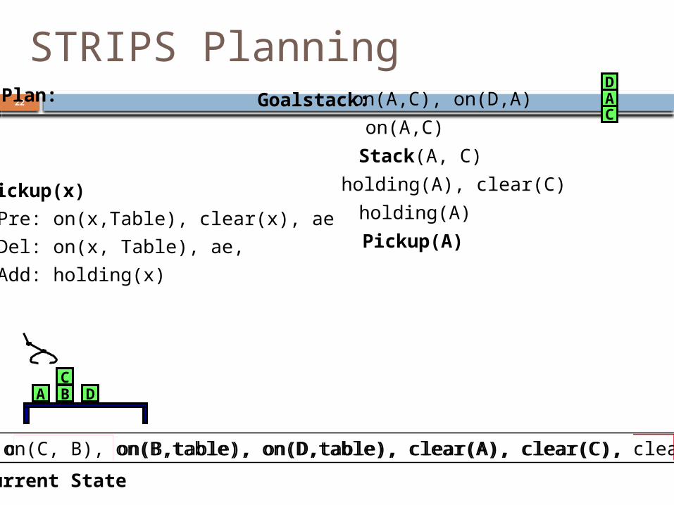
22



Current State

Plan: Goalstack:

on(A,C)

Stack(A, C)

holding(A), clear(C)

holding(A)

Pickup(A)

ACB D

CAD

Pickup(x)

Pre: on(x,Table), clear(x), ae

Del: on(x, Table), ae,

Add: holding(x)

holding(A), on(C, B), on(B,table), on(D,table), clear(A), clear(C), clear(D).

23

STRIPS Planning

holding(A), on(C, B), on(B,table), on(D,table), clear(A), clear(C), clear(D).

on(A,C), on(D,A)

Current State

Plan: Goalstack:

on(A,C)

Stack(A, C)

A

CB D

CAD

Stack(x, y)

Pre: holding(x), clear(y)

Del: holding(x), clear(y)

Add: on(x, y), ae

Pickup(A)

on(A,C), on(C, B), on(B,table), on(D,table), clear(A), clear(D), ae.

24


on(A,C), on(C, B), on(B,table), on(D,table), clear(A), clear(D), ae.

Current State

Plan: Goalstack:

on(D, A)

Stack(D,A)

holding(D), clear(A)

holding(D)

Pickup(D)

on(D,Table), clear(D), ae

ACB D

CAD

on(A,C), on(C, B), on(B,table), holding(D), clear(A), clear(D)on(A,C), on(C, B), on(B,table), on(D,A), clear(A), ae

Stack(A, C)

Pickup(A)

25


Current State

Plan: Goalstack:

on(D, A)

Stack(D,A)


holding(D)

Pickup(D)

ACB

D

CAD

on(A,C), on(C, B), on(B,table), holding(D), clear(A), clear(D)on(A,C), on(C, B), on(B,table), on(D,A), clear(A), ae

Stack(A, C)

Pickup(A)

26

STRIPS Planning: Getting it Wrong!on(A,C), on(D,A)


Current State

Plan: Goalstack:

on(D,A)

Stack(D, A)


holding(D)

Pickup(D)

on(D,Table), clear(D), ae

ACB D

CAD

on(A,table), on(C, B), on(B,table), holding(D), clear(A), clear(C), clear(D)

27

STRIPS Planning: Getting it Wrong!

on(A,table), on(C, B), on(B,table), holding(D), clear(A), clear(C), clear(D)

on(A,C), on(D,A)

on(A,table), on(C, B), on(B,table), on(D,A), clear(C), clear(D), ae.

Current State

Plan: Goalstack:

on(D,A)

Stack(D, A)

Pickup(D)

ACB

D

CAD

28

STRIPS Planning: Getting it Wrong!

on(A,C), on(D,A)

on(A,table), on(C, B), on(B,table), on(D,A), clear(C), clear(D), ae.

Current State

Plan: Goalstack:

Stack(D, A)

Pickup(D)

ACB

D

CAD

Now What?– We chose the wrong goal first– A is no longer clear.– stacking D on A messes up the preconditions for

actions to accomplish on(A, C)– either have to backtrack, or else we must undo

the previous actions

29

STRIPS planning (Goalstack planning)

Works on one subgoal at a time Insists on completely achieving that

subgoal before considering other subgoals May have to backtrack:

If it chooses the wrong order to work on the subgoals

If it chooses the wrong action to achieve a subgoal

Searches backwards from goal – uses goal to guide choice of actions

30

Limitation of state-space search

Linear planning or Total order planning Example

Initial state: all the blocks are clear and on the table

Goal: On(A,B) Λ On(B,C) If search achieves On(A,B) first, then needs

to undo it in order to achieve On(B,C) Have to go through all the possible

permutations of the subgoals

31

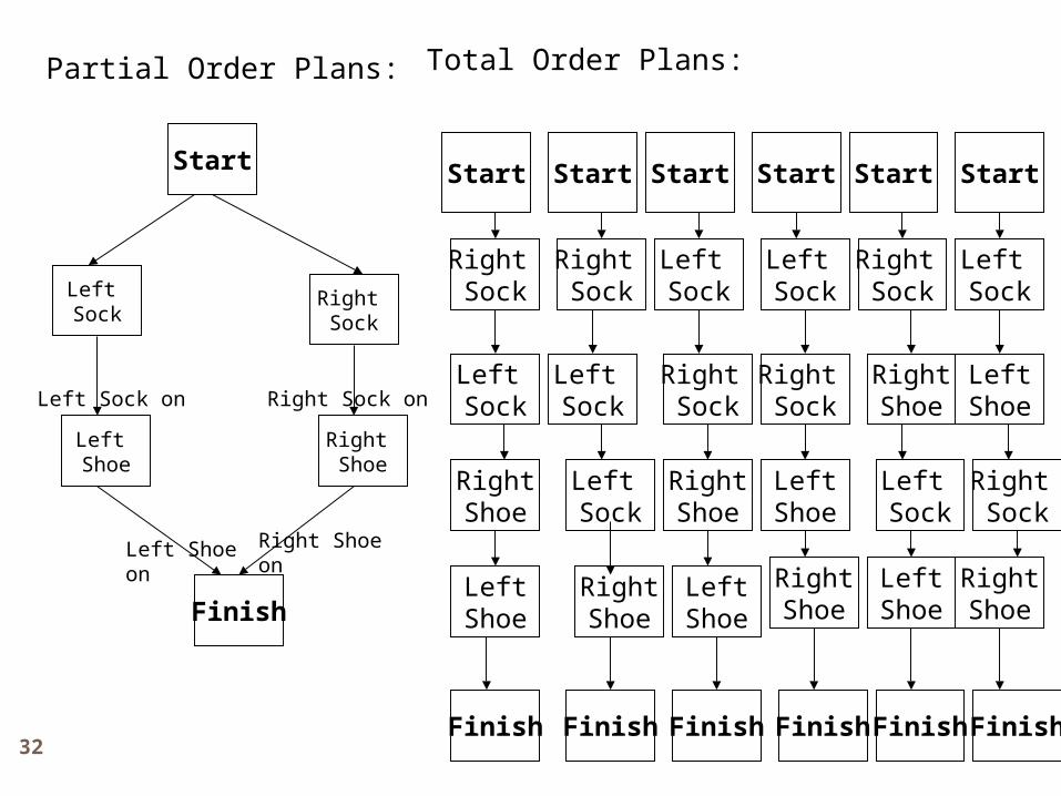
Search through the space of plans

Nodes are partial plans, links are plan refinement operations and a solution is a node (not a path).

This can be powerful if the plan representation and refinements change the search space.

POP creates partial-order plans following a “least commitment” principle.

32

Left Sock

Start

Finish

Right Shoe

Left Shoe

Right Sock

Start

Right Sock

Finish

LeftShoe

RightShoe

Left Sock

Start Start Start Start Start

Right Sock

Right Sock

Right Sock

Right Sock

Right Sock

Left Sock

Left Sock

Left Sock

Left Sock

Left Sock

Left Sock

RightShoe

RightShoe

RightShoe

RightShoe

RightShoe

LeftShoe

LeftShoe

LeftShoe

LeftShoe

Finish Finish Finish Finish Finish

Left Shoe on Right Shoe on

Left Sock on Right Sock on

Partial Order Plans: Total Order Plans:

33

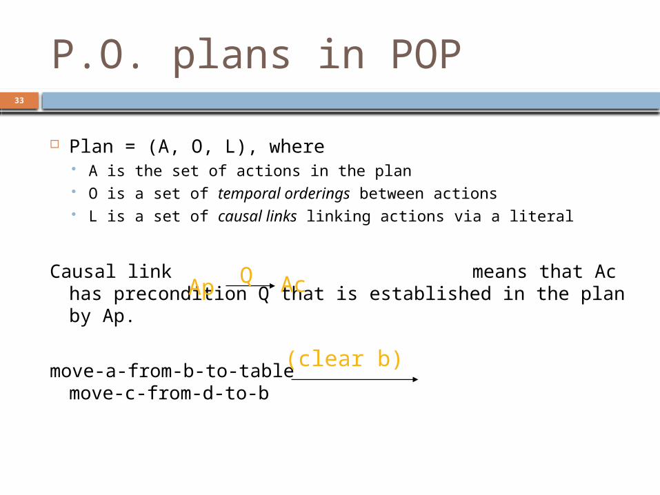
P.O. plans in POP

Plan = (A, O, L), where A is the set of actions in the plan O is a set of temporal orderings between actions L is a set of causal links linking actions via a literal

Causal link means that Ac has precondition Q that is established in the plan by Ap.

move-a-from-b-to-table move-c-from-d-to-b

Ap AcQ

(clear b)

34

Threats to causal links

Step At threatens link if:1. At has (~Q) as an effect2. At could come between Ap and Ac, i.e., O

is consistent with Ap < At < Ac

Ap AcQ

35

Threat Removal

Threats must be removed to prevent a plan from failing

Demotion adds the constraint At < Ap to prevent clobbering, i.e. push the clobberer before the producer

Promotion adds the constraint Ac < At to prevent clobbering, i.e. push the clobberer after the consumer

36

Initial (Null) Plan

Initial plan has A = { A0, A¥} O = {A0 < A¥} L = {}

A0 (Start) has no preconditions but all facts in the initial state as effects.

A¥ (Finish) has the goal conditions as preconditions and no effects.

37

POP algorithmPOP((A, O, L), agenda, PossibleActions):1. If agenda is empty, return (A, O, L)2. Pick (Q, An) from agenda3. Ad = choose an action that adds Q.

a. If no such action exists, fail.b. Add the link Ad Ac to L and the ordering Ad < Ac to Oc. If Ad is new, add it to A.

4. Remove (Q, An) from agenda. If Ad is new, for each of its preconditions P add (P, Ad) to agenda.

5. For every action At that threatens any link 1. Choose to add At < Ap or Ac < At to O.2. If neither choice is consistent, fail.

6. POP((A, O, L), agenda, PossibleActions)

Q

Ap AcQ

38

Sussman Anomaly

A0(on C A) (on-table A) (on-table B) (clear C) (clear B)

A ¥

(on A B) (on B C)(on-table C)

39

Work on open precondition (on B C)


A ¥

(on A B) (on B C)

A1: move B from Table to C

(on B C)-(on-table B) -(clear C)

(clear B) (clear C) (on-table B)

(on-table C)

40

Work on open precondition (on A B)


A ¥

(on A B) (on B C)



(clear B) (clear C) (on-table B)A2: move A from Table to B

(clear A) (clear B) (on-table A)

(on A B)-(on-table A) -(clear B)

(on-table C)

41

Work on open precondition (on-table C)


A ¥

(on A B) (on B C)



(clear B) (clear C) (on-table B)

A2: move A from Table to B

(clear A) (clear B) (on-table A)

(on A B)-(on-table A) -(clear B)

A3: move C from A to Table

(clear C)(on C A)

-(on C A)(on-table C) (clear A)

(on-table C)

42

Analysis

POP can be much faster than the state-space planners because it doesn’t need to backtrack over goal orderings (so less branching is required).

Although it is more expensive per node, and makes more choices than RegWS, the reduction in branching factor makes it faster, i.e., n is larger but b is smaller!

43

More analysis

Does POP make the least possible amount of commitment?

Lifted POP: Using Operators, instead of ground actions,

Unification is required

44

POP in the Blocks world

On(x,y), Cl(x), ~Cl(y), ~On(x,z)

PutOn(x,y)

Cl(x), Cl(y), On(x,z)

PutOnTable(x)

On(x, z) Cl(x)

On(x,Table), Cl(x), ~On(x,z)

45


46


47


48


49

Example 2

A0: Start At(Home) Sells(SM,Banana) Sells(SM,Milk)

Sells(HWS,Drill) A¥ : Finish

Have(Drill) Have(Milk) Have(Banana) At(Home)

Have(y)

Buy (y,x)

At(x), Sells(x,y)

GO (x,y)

At(x) At(y) ~At(x)

50

POP Example

finish

start

51

POP Example

finish

start

Have(M) Have(B)

Sells(SM, M) Sells(SM,B) At(H)

52

POP Example

finish

start

Have(M)

Buy (M,x1)

At(x1) Sells(x1,M)

Have(M) Have(B)


53

POP Example

finish

start

Have(M)

Buy (M,x1)

At(x1) Sells(x1,M)

Have(M) Have(B)


54

POP Example

finish

start

Have(M)

Buy (M,x1)

At(x1) Sells(x1,M)

Have(M) Have(B)


55

POP Example

finish

start

Have(B)Have(M)

Buy (M,x1)

At(x1) Sells(x1,M)

Buy (B,x2)

Have(M) Have(B)

At(x2) Sells(x2, B)


56

POP Example

finish

start

Have(B)Have(M)

Buy (M,x1)

At(x1) Sells(x1,M)

Buy (B,x2)

Have(M) Have(B)

At(x2) Sells(x2, B)


57

POP Example

finish

start

Have(B)

x1 = SM

Have(M)

Buy (M,x1)

At(x1) Sells(x1,M)

Buy (B,x2)

Have(M) Have(B)

At(x2) Sells(x2, B)


58

POP Example

finish

start

Have(B)

x1 = SM

Have(M)

x2 = SM

Buy (M,x1)

At(x1) Sells(x1,M)

Buy (B,x2)

Have(M) Have(B)

At(x2) Sells(x2, B)


59

POP Example

finish

start

Have(B)

x1 = SM

Have(M)

x2 = SM

GO (x3,SM)

At(x3)

At(SM)

Buy (M,x1)

At(x1) Sells(x1,M)

Buy (B,x2)

Have(M) Have(B)

At(x2) Sells(x2, B)


60

POP Example

finish

GO (x3,SM)

start

Have(B)

x1 = SM

Have(M)

x2 = SM At(x3)

At(SM)

Buy (M,x1)

At(x1) Sells(x1,M)

Buy (B,x2)

Have(M) Have(B)

At(x2) Sells(x2, B)


61

POP Example

finish

GO (x3,SM)

start

Have(B)

x1 = SM

Have(M)

x2 = SM At(x3)

At(SM)

Buy (M,x1)

At(x1) Sells(x1,M)

Buy (B,x2)

Have(M) Have(B)

At(x2) Sells(x2, B)


62

POP Example

finish

GO (x3,SM)

start

Have(B)

x1 = SM

Have(M)

x2 = SM At(x3)

At(SM)

x3 = H

Buy (M,x1)

At(x1) Sells(x1,M)

Buy (B,x2)

Have(M) Have(B)

At(x2) Sells(x2, B)


63

POP Example

finish

GO (x3,SM)

start

Have(B)

x1 = SM

Have(M)

x2 = SM At(x3)

At(SM)

x3 = H

Buy (M,x1)

At(x1) Sells(x1,M)

Buy (B,x2)

Have(M) Have(B)

At(x2) Sells(x2, B)


1 07. The planning problem 2 Inputs: 1. A description of the world state 2. The goal state...

Documents

Transcript of 1 07. The planning problem 2 Inputs: 1. A description of the world state 2. The goal state...