08-DataAcquisition

8/6/2019 08-DataAcquisition

http://slidepdf.com/reader/full/08-dataacquisition 1/20

Panorama Technologies

Chapter 8Data Acquisition

This chapter describes the principal ways in which data acquisition aects the seismicdata processing eort. This includes information about array eects, aperture, aliasing,and the physical arrangement of the acquisition methods themselves.

It may be that the most frequently asked question about seismic acquisition is aboutthe optimum approach to seismic acquisition. Fundamentally this is a question aboutthe geometry and sampling rate of the receiver array, but it easily expands to includewhat source we should use, what microphones we should employ, whether or not weshould use geophone sub-arrays, how big our aperture should be, and, nally, whattemporal and spatial sampling rates we should select. In the spatial sense, we havealways acquired seismic data digitally. We never had continuous (analog) sampling inspace; analog data was only acquired in time.

The answers to these questions are mathematically and physically clear. For eachsource, the receiver array should consist of point receivers (no arrays) densely sampledover a wide aperture array encompassing a large square area. The source, howeverit is formed, should be a point source (no arrays) generating energy uniformly in alldirections. For maximum benet, there should be full source-receiver reciprocity; thatis, for each receiver position, there should be a source, and for each source there shouldbe a receiver. Hopefully, this chapter will make the reason for these statements clear.

Unfortunately, there are many reasons why the mathematics and physics are almost

always ignored—primarily, economics and practicality trump correctness. Furthermore,faced with budget limitations in an era when oil was relatively easy to nd, littleor no consideration was given to the underlying mathematical assumptions. Manygeophysicists assumed that mathematics, including the wave equation, did not applyto the seismic acquisition process. Arrays were designed to control perceived noise,but frequently depressed the dip response. Fancy acquisition geometries were designedto reduce costs, but resulted in data sets that could not image geologic objectives.Illumination studies were conducted in an attempt to determine the impact of any given

229



Array Effects Panorama Technologies

acquisition style, but, because they were often based on one-way equations or rays, thestudies had no real impact on the solution—such studies can be fairly meaningless sincecomplicated waveforms exist in even relatively simple geologic environments.

In contrast, mathematics does not lie. Mathematics, physics and a tremendous amount of

empirical evidence suggests that imaging is a complex process almost totally controlledby the degree to which mathematical assumptions are honored. While we will not gointo the mathematics in detail, we hope to provide a reasonable clarication of whywe should acquire data in a precise, mathematically-correct manner. We will show thatacquisition schemes can and should be modied to meet implicit assumptions.

Array Effects

Instead of recording single, non-overlapping shots into straight-line arrays, acquisitionbecame one in which each shot was recorded by a line of receivers laid out on eitherside of the central shot. When receivers are laid out on only one side of a source, theresulting acquisition is said to be single ended. Figure 8-1 shows a typical single-endedacquisition, where a modern land vibrator provides the energy source causing thesubsurface waveeld and its reection. Receiver arrays record the response.

Figure 8-1. Schematic of typical multi-fold, single-end seismic recording process

The bottom part of this gure shows how receiver arrays can be arranged and summedto produce a single trace. The output of this sub-array forces us to recognize that eachtrace can be aected by the array response. Although such arrays were supposed toreduce noise when it was not economically feasible to record the full output at eachlocation, the mathematics says we should record and image using all receivers.

230 Modeling, Migration and Velocity Analysis



Panorama Technologies Array Effects

Array eects are rarely considered as part of the overall acquisition-data processing-imaging methodologies. In fact, the underlying mathematics is based on the assumptionthat each receiver is a so-called point receiver, but this assumption is wrong when anarray is involved. Figure 8-2 demonstrates the smearing that arrays cause. The threeimages show the eect of recording every trace, a group of 8 traces, and a group of 16

traces. Note the considerable blurring caused by the mixing. While it appears to improvecontinuity and reduce noise, the net eect tends to be unwanted dip reduction.

Figure 8-2. The effect of seismic arrays.

Among other things, smearing can reduce the dip response of the recording systemand thereby seriously decrease the quality of the ultimate image. Although it seemslike a good idea to use arrays, and, when steep dips are not an issue, it seems to make

sense, that is never really the case. The use of arrays is a fundamental violation of themathematical assumptions in all cases. Today, it is probably possible to record all thereceivers. The aect of any given array can be emulated in the processing stage, soapplying it in the eld seems to be unnecessary and it is perhaps a big mistake.

Chapter 8. Data Acquisition 231



Aperture Panorama Technologies

Aperture

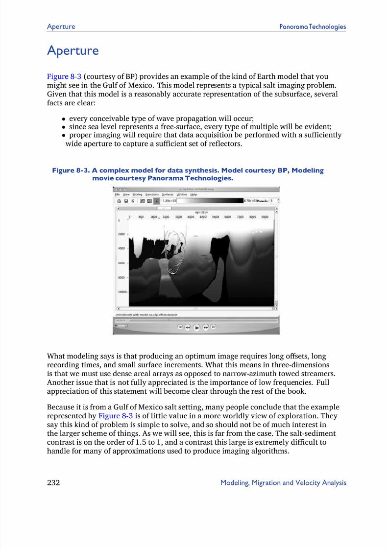
Figure 8-3 (courtesy of BP) provides an example of the kind of Earth model that youmight see in the Gulf of Mexico. This model represents a typical salt imaging problem.

Given that this model is a reasonably accurate representation of the subsurface, severalfacts are clear:

• every conceivable type of wave propagation will occur;• since sea level represents a free-surface, every type of multiple will be evident;• proper imaging will require that data acquisition be performed with a suciently

wide aperture to capture a sucient set of reectors.

Figure 8-3. A complex model for data synthesis. Model courtesy BP, Modelingmovie courtesy Panorama Technologies.

What modeling says is that producing an optimum image requires long osets, longrecording times, and small surface increments. What this means in three-dimensionsis that we must use dense areal arrays as opposed to narrow-azimuth towed streamers.

Another issue that is not fully appreciated is the importance of low frequencies. Fullappreciation of this statement will become clear through the rest of the book.

Because it is from a Gulf of Mexico salt setting, many people conclude that the examplerepresented by Figure 8-3 is of little value in a more worldly view of exploration. Theysay this kind of problem is simple to solve, and so should not be of much interest inthe larger scheme of things. As we will see, this is far from the case. The salt-sedimentcontrast is on the order of 1.5 to 1, and a contrast this large is extremely dicult tohandle for many of approximations used to produce imaging algorithms.




Panorama Technologies Aperture

Figure 8-4 provides an example of the kind of complex geology we nd on land. Thisperceived Oklahoma subsurface model from an over-thrust area in the southwestern partof the state faithfully represents a granitic overthrust in a very complex geologic setting.Once again, modeling tells us that to properly image subsurface structure, it is absolutelynecessary to acquire long osets and times. Thus, in both land and marine, satisfying

mathematical assumptions means that acquisition arrays must be composed of pointreceivers, they must be areal in extent, and they must be densely sampled.

Figure 8-4. A complex model for data synthesis. Model courtesy ChesapeakeEnergy, Modeling movie courtesy Panorama Technologies.

The rocks are hard, the near surface velocity is highly variable, and it is not unrealistic toassume that the true Earth model should really include anisotropy. Again, all waveformsare present in the simulation, and unraveling them requires that, to the extent possible,all waveforms be used in the imaging.

A big dierence between imaging land and marine data is the lack of water cover for

land data. When water is present, it is relatively easy to gure out what the near surfacepropagation parameters should be since it is not necessary to rely on the recorded datato determine the velocity of water. When water is not present, we must estimate thenear surface velocity structure (compressional and shear) from the data itself, but thisis very dicult to do because the number of traces that can be used to do this is highlyrestricted by the acquisition parameters. Sucient oset is seldom available to do evensimple semblance-based picking. What modern methods need is data that are t forpurpose; data must contain the information necessary to permit accurate estimation of the Earth model.




Aliasing Panorama Technologies

Aliasing

Aliasing happens when the frequency of repetition is too fast for the true nature of the repetition to be recognized. For example, everyone who has ever watched an old

American Western movie has seen wagon wheels, maybe like those in Figure 8-5, spindiametrically opposed to the direction of travel (backwards). This occurs because thethirty-frame per second sampling rate of the movie camera is incapable of resolving thefaster rate of the wheel spin. The net result is that the wheel appears to spin at a slowerrate in the wrong (backwards) direction.

Figure 8-5. Wheels alias when in motion.

For our purposes, spatial aliasing in seismic exploration makes it impossible to correctly

distinguish and image dipping events at their true position and angle. Many peopleargue that the mathematics of sampling is incorrect because they believe that if thehuman eye can recognize the correct pattern, the more mathematical migrationalgorithms should also be able to do so. But our brains make the event appearcontinuous, and handles it from there, while discrete mathematics cannot do this. Themathematics of discrete migration algorithms make strong demands on what kind of datathey can handle because they cannot make the data continuous before they process it.Consequently, both acquisition design and the imaging algorithm must take aliasing intoaccount. In some cases, the algorithm can be designed to handle any aliasing problemor issue automatically and directly. However, when this is not the case, aliasing mustbe avoided during the acquisition process itself. The elimination of aliasing ensures that

dipping events are imaged as optimally as possible.

Data acquisition parameters play an important role in subsequent imaging exercises,while imaging algorithms vary considerably in their sensitivity to acquisition parameters.Understanding the impact of acquisition parameters on imaging techniques is the key toproducing superior images.

Many geophysicists believe that there is some magic level of sampling, or that thesampling rules seemingly demanded by acquisition and processing are unnecessarily




Panorama Technologies Aliasing

strict. The basic idea that the human eye is better than the computer at being able tosee through under-sampled data is probably true. However, ensuring that any givenimaging application produces the most optimum results limits both the kind and styleof the acquisition method. For the most part, data must be sampled suciently nely toensure that the imaging algorithm can image target objects without loss of dip or image

quality.

Figure 8-6 provides simple, conservative formulas relating the important parametersthat aect the relationship of dipping reectors at their true subsurface position to theirapparent dip on a two-dimensional seismic recording when the source and receiversare coincident and the velocity is constant. The relationship between apparent dip, asspecied by a change in time versus a change in space, coupled with Shannon’s samplingtheorem, tells us when to expect and how to handle potential aliasing caused by spatialsampling intervals.

Figure 8-6. Aliasing Formulas

The trigonometric function of the true dip of the subsurface event turns out to be theratio of half of the relative change in two-way time of the event at its apparent position,

, to the spatial range over which the time change takes place, , multiplied by theassumed constant velocity of sound in the medium.

After this simple concept is understood, it is straightforward to use the Nyquistrelationship between time sampling and frequency to rewrite the basic formula interms of frequency. The Nyquist relationship states that a signal must be sampled ata rate greater than twice the highest frequency component of the signal to accuratelyreconstruct the waveform; otherwise, the high-frequency content will alias at a frequencyinside the spectrum of interest.





Note that xing any three parameters in the variety of formulas rewriting the basicformula produces provides a bound for the fourth. In 3D, it is important to do thecalculations based on the largest spatial interval in the data set, Thus, if we want tomake sure that we can image a given set of dips at a given frequency and velocity, wemust make sure that the data has been recorded at the correct spatial spacing, or we

must migrate it at the proper sampling interval.

You should understand that these are conservative formulas. The fact that velocities varyhelps the imaging process because, in this kind of medium, ray bending improves theability to image steeper dips. In precise mathematical terms, note that:

(8-1)

=

=

2sin

We all claim to understand the idea that when we sample a signal at a xed evenincrement, the resulting set of samples can be used to reconstruct the original signal

completely, but only up to a xed frequency determined by the sampling rate (that is,the Nyquist frequency). Thus, if we sample at 250 samples per second (in other words,4 milliseconds per sample), the highest possible frequency we can record correctly is125 Hz, or exactly half the sampling rate. Note that in this case, the Nyquist frequencyis determined equally from 250 or half of 1.0/.004. Thus, 125 = 1.0/.008. A similarequivalence is available for surface sampling parameters. If lines are spaced at 100meters, the spatial Nyquist frequency in the line direction is 1.0/200. This Nyquistfrequency species the maximum wavenumber or wavelength that can be safelyrecovered from the surface sampled data in the line direction.

Figure 8-7 shows a schematic of a single plane monochromatic wave front traveling

at a slight angle relative to the vertical. The wave front on the right is recordedin time, while that on the left is recorded in depth. The wave front in this case ispropagating in a constant velocity medium and is characterized by its vertical andhorizontal wavenumbers, or their reciprocal wavelengths. The vertical wavenumber,, is completely determined by the frequency, , and the velocity, . In contrast, thehorizontal wavenumber, , is impacted by the angle of propagation. Later, we will seethat this dependence on angle can be used to specify a simple migration algorithm.




Panorama Technologies Aliasing

Figure 8-7. Wavenumbers

Figure 8-7 also shows the relationship between monochromatic wavefronts true dip.The gure shows how the trigonometric functions relating apparent dip to true dip areexpressed in the frequency domain. The most important formulas say that the sine of thetrue dip angle, , is equal to the tangent of the apparent dip angle, .

It is important to note that in the real world, this means that we must consider measuredseismic data to be digital in character, since the sources and receivers are at discretelocations. Since modern data is also digital in time, reection seismic processing todayis purely digital. Since wavenumbers of plane waves carry information about the angleof propagation, this suggests that there will be some issues with regard to the aliasing of

dipping subsurface reectors. The impact of aliasing on our ability to image subsurfaceevents will be discussed in subsequent sections.

Aliasing appears in many ways. Figure 8-8 demonstrates the appearance of aliasingon zero oset sections. Here we see the dierence between sampling at 27.5 feet and110 feet. The gure on the left at 27.5 feet is clearly less aliased than the one on theright at 110 feet; that is, the section on the left has been sampled suciently nely toalmost completely eliminate all aliasing for this level of dip. The section on the right wasconstructed by simply eliminating traces from the one on the left. Evidence of aliasingis represented by the grainy appearance and by the areas where events that follow somehyperbolic-like trajectory appear more like a single at event.





Figure 8-8. Aliasing when the data are flat.

The synthetic CDP in Figure 8-9 is a normal moveout corrected CDP or midpoint

gather with both at and hyperbolic arrivals. It demonstrates a form of aliasing thatoccurs when the moveout of an event is so strong that the recorded spatial samplingcannot handle its rapidity adequately. This means that events can be aliased in oseteven when all dips are perfectly sampled in space. This gure shows a synthetic(raytraced) CDP with multiples that are aliased in oset. While the human eye has nodiculty recognizing the pattern of these events, many noise suppression and migrationalgorithms will treat these events in a predictable, but incorrect manner. For example, aRadon transform is not be able to completely remove the event from the record.

Figure 8-9. Offset aliasing.




Modern Acquisition Geometries Panorama Technologies

acquisition produces data sets with uniform surface coverage. Because the number of recording lines is small, it usually only produces narrow azimuth data.

As was the case for our split-spread acquisition, each gather from either of the recordinggeometries in Figure 8-10 can be migrated independently of any other similar gather.

Thus, we can conceive of migrating common azimuth volumes for detailed illuminationcomparisons. Note that this kind of acquisition produces ve dimensional data sincethere are two coordinates for the source, two coordinates for the receiver, and onecoordinate for time. The most important point is that widely spaced lines are good forquick coverage but are bad for spatial sampling.

Sampling will become an issue later when we discuss its impact on high resolutionmigration algorithms. Although this style of sampling can generate many dierentazimuths, each azimuth is poorly sampled, meaning that, in some cases, azimuthmigration cannot be performed.

CATS, NATS, and WATS

Marine data acquisition has evolved from single cable, single source acquisition to multi-cable multiple source, multiple boat and even ocean bottom (OBC) congurations thatcan record long oset data in record time. Again, redundant coverage can be sorted intoany of the orders discussed in old-fashioned, split-spread shooting.

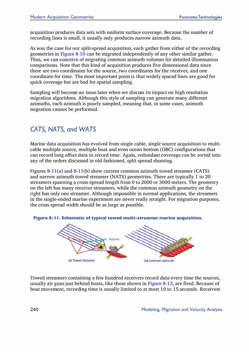
Figures 8-11(a) and 8-11(b) show current common azimuth towed streamer (CATS)and narrow azimuth towed streamer (NATS) geometries. There are typically 1 to 20streamers spanning a cross-spread length from 0 to 2000 or 3000 meters. The geometryon the left has many receiver streamers, while the common azimuth geometry on theright has only one streamer. Although impossible in normal applications, the streamersin the single-ended marine experiment are never really straight. For migration purposes,the cross-spread width should be as large as possible.

Figure 8-11. Schematic of typical towed multi-streamer marine acquisition.

Towed streamers containing a few hundred receivers record data every time the sources,usually air guns just behind boats, like those shown in Figure 8-12, are red. Because of boat movement, recording time is usually limited to at most 10 to 15 seconds. Receivers




Panorama Technologies Modern Acquisition Geometries

in each streamer data are very nely sampled in each dimension. Cable spacing israrely more than 100 meters with the number of cables ranging between 1 and 20. Thenumber of traces per shot is large while the shot density per unit area can be relativelylow. Although this kind of geometry has been used for many years and has provento be reasonably good for advanced imaging techniques, it is still somewhat far from

what the mathematics and physics demands. An important issue with this approach iscable feathering caused by water currents, which usually means that it is not possibleto achieve the precise common azimuth form shown in the right half of Figure 8-11.Since most of the algorithms we consider must be run on a grid, traces may have to beregularized to that grid to ensure algorithm accuracy and nal image quality.

Figure 8-12. Schlumberger (Western Geophysical, GECO) boats in operation. Notethe towed streamers and the triangular shape of the Ramform gunboats.





Figure 8-13(a) and (b) show a wide angle towed streamer (WATS) acquisition andcomposite shot. In WATS schemes, gunboats make multiple passes over the same shotline. One gunboat is placed at the head and to one side of the receiver array and theother is on the same side at the end of the array. The boat towing the receiver arrayparallels the gunboats, but traverses an every widening path in accordance with each

pass of the source boats. Part (a) shows double gunboats recorded by a single eightstreamer receiver boat to achieve shot centered receiver arrays. Four or more widerreceiver swaths may have to be recorded to produce sucient data to produce receiverarrays with areal coverage, as indicated by the surface coverage in the composite shotlayout in Part (b). The WATS technology may be the rst marine acquisition scheme thatactually honors the mathematical assumptions underlying seismic imaging algorithms.

Figure 8-13. The geometry of wide azimuth towed streamer acquisition.

(a). Wide azimuth towed streameracquisition

(b). Wide azimuth towed streamercomposite shot

The composite shot in Figure 8-13(b) can contain a huge number of receivers. This gurewas constructed based on the assumption that the receiver boat could eectively tow justeight streamers. Utilization of receiver boats towing 16 or more streamers would cut thework load signicantly while still producing a composite shot that is much closer to thetrue mathematical ideal. When 8,000 meter streamers are separated by 100 meters, eightstreamer WATS shots have an areal extent of approximately 6,000 meters by 16,000meters but could certainly cover an area 16,000 meters on a side. As shown by BP, thesetypes of acquisitions do, in fact, produce data sets fully capable of imaging complexsubsurface geology.

Vertical Cables (VC)

Vertical cables, as shown in Figure 8-14, are just that. Receivers are actually placedalong a vertical cable suspended at a xed surface location either by sea anchors orby a tether attached to the ocean bottom. Usually source and receiver reciprocity isused to change the acquisition process into an equivalent one where the sources are





assumed to be along the cable and the receivers on the surface. While vertical cableacquisition is certainly capable of generating the equivalent of the composite shots of WATS, this particular approach has never achieved its promise, probably because of the inability to keep the cable in a xed and completely vertical position. Furthermore,processing common receiver gathers as if they were common source gathers is much

more computationally ecient than processing common-shot gathers.

Figure 8-14. Marine Vertical Cable Acquisition.

Ocean Bottom (OBC)

Since gunboats can shoot in a virtually unlimited set of locations, OBC acquisition cangenerate areal array shots quite easily. In Figure 8-15, receivers are laid on the ocean

bottom and sources are located on the surface in gun boats like those shown in Figure 8-16. The receivers on the ocean bottom can be organized into a grid or as a small set of cables similar to those used on the surface. The grid can be positioned on the bottom bya remotely operated vehicle, by a manned submersible, or by simply allowing the cablesor receiver unit to sink to the bottom. Wireless communication can be used to accuratelylocate the receivers when in position.

Figure 8-15. Schematic of a typical ocean bottom acquisition.





Figure 8-16. Fairfield gunboats near shore. OBC acquisition removes many restrictions on where source boats can sail.

Because the sources are at the surface, the gun boat can move in any direction desired.As a result, many azimuths can be recorded during the acquisition session. Data fromthe receivers can be recorded on the gun boat or on another boat especially designedfor recording and processing. If sea-oor cables are used, this acquisition can be verysimilar to orthogonal shooting on land. The basic dierence is that the source boat

can move in any desired direction and consequently can generate full azimuth surveys.Usually source-receiver reciprocity is used to view a common-receiver gather as a singleshot, making source spacing and density extremely important. Because receivers areactually on the ocean bottom, this data usually must be preprocessed almost as if it wasland data. Certainly, receiver coupling or lack thereof, and the consequent amplitudedierences must be addressed and eliminated or at least suppressed.

Regardless of how they are generated, seismic waveelds are the result of particlemotion in the medium. Figure 8-17 shows two types of motion: compressional andshear. The red wavefront particles are vibrating tangentially to the wavefront as partof a shear wave. In a medium where velocity varies with angle (that is, an anisotropic

medium), there are two orthogonal shear waves. Shear waves do not propagate in a uidor gas. Particles on the blue wavefront vibrate perpendicular to the wavefront in the raydirection and consequently are part of a compressional wave. Perhaps the best exampleof a compressional wave is sound in air. Particles in air are compressed and raried asthe wave front progresses. Compressional waves travel in virtually all uids and solids.Shear waves in solids generally travel at about 60% of the speed of compressional waves.Typical speeds of compressional waves are 330 m/s in air, 1450 m/s in water and about5000 m/s in granite.





Figure 8-17. Shear versus Compressional waves

Shear waves are much more dicult to visualize than compressional waves. A good wayto think of shear propagation is to consider a deck of cards. It is quite easy to slide thecards in the deck against each other and so generate a wave that propagates through thedeck from one end to the other. While this is not necessarily how such waves propagatein the earth, the existence of shear propagation is not in question. Since shear wavescannot propagate in water, it is impossible to record shear waves in the water layer, butthis does not mean that marine recordings do not contain shear wave information sinceall recordings, both land and marine, contain converted wave data. Seismic data fromland and OBC data can both contain direct shear reections, but data recorded in watercontains only shear-related compressional waves that are direct conversions from shearto compressional at the water-ocean-bottom interface.

Practical acquisition of OBC data, as shown in Figures 8-18, 8-19, and 8-20 takesseveral forms. Whether the receivers are cables, as shown in Figure 8-18, or individualunits like those shown in Figures 8-19 and 8-20, the primary objective is to place the

receivers on the ocean bottom at precisely known locations, but this is not always easyto do. For example, cables are usually towed and then dropped, but even with radiosensors, it is not always possible to determine their exact ocean bottom position. Theunits in Figures 8-19 and the more modern version in Figure 8-20 contain computersystems that can accurately determine position and relay the information back to therecording instruments. In addition, they have sucient local storage to record severalshot responses before they must transmit the data to the primary storage system.

Figure 8-18. Ocean bottom layout and acquisition. This figure shows the cablesand sensors used to acquire data from ocean bottom cables.





Figure 8-19. This figure shows boxlike ocean bottom receivers being deployedoverboard (bottom left and top right) in both deep and shallowmarine environments. The top left composite demonstrates thatsource boats can operate close to shore and platforms.

Figure 8-20. Fairfield Industries’ latest ocean bottom recorder contains fourphones and all the electronics necessary to record source-responses.

The secondary objective of OBC recording is to ensure that each component of theOBC receiver is correctly oriented. Each OBC phone contains a hydrophone, twoshear phones, and one accelerometer. The two shear phones must be level and theirorientation xed relative to the rest of the receiver units. Consequently, they are

gimbaled and adjustable based on each unit’s digital compass. Clearly, OBC acquisitionis dicult and potentially expensive.

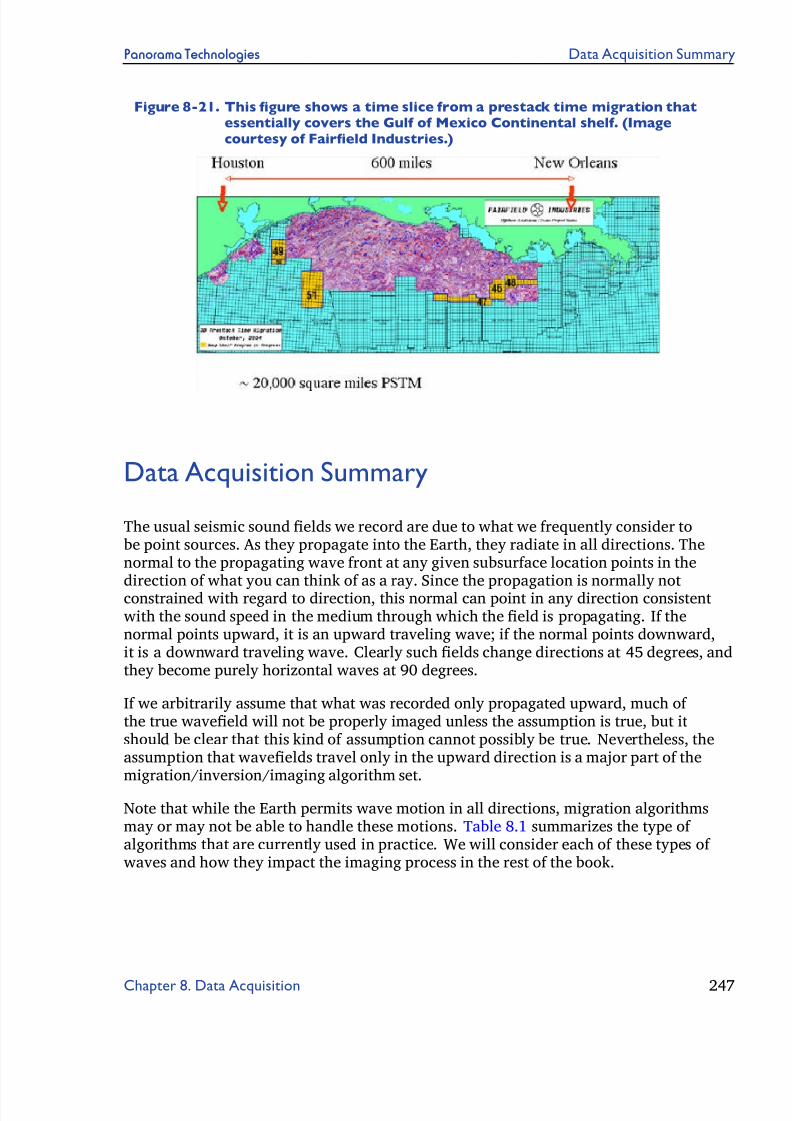
Regardless of which acquisition method is employed, the net result are data volumes thatare truly massive. Figure 8-21 shows a single time slice through 20,000 square milesof prestack, time-migrated Gulf of Mexico data with an average redundancy of about90. Simple back of the envelope calculations suggest that the size of this data volumeis several hundred terabytes or more. One can easily imagine ocean bottom acquisitionsmore than four times as large as this one.




Panorama Technologies Data Acquisition Summary

Figure 8-21. This figure shows a time slice from a prestack time migration thatessentially covers the Gulf of Mexico Continental shelf. (Imagecourtesy of Fairfield Industries.)

Data Acquisition Summary

The usual seismic sound elds we record are due to what we frequently consider tobe point sources. As they propagate into the Earth, they radiate in all directions. Thenormal to the propagating wave front at any given subsurface location points in thedirection of what you can think of as a ray. Since the propagation is normally notconstrained with regard to direction, this normal can point in any direction consistentwith the sound speed in the medium through which the eld is propagating. If thenormal points upward, it is an upward traveling wave; if the normal points downward,it is a downward traveling wave. Clearly such elds change directions at 45 degrees, andthey become purely horizontal waves at 90 degrees.

If we arbitrarily assume that what was recorded only propagated upward, much of the true waveeld will not be properly imaged unless the assumption is true, but itshould be clear that this kind of assumption cannot possibly be true. Nevertheless, theassumption that waveelds travel only in the upward direction is a major part of themigration/inversion/imaging algorithm set.

Note that while the Earth permits wave motion in all directions, migration algorithmsmay or may not be able to handle these motions. Table 8.1 summarizes the type of algorithms that are currently used in practice. We will consider each of these types of waves and how they impact the imaging process in the rest of the book.




Data Acquisition Summary Panorama Technologies

Table 8.1. Wave Motion Hierarchy

Wave Motion Wave Type

Waves move in all directions Two-way wave motionTurning waves and rays

Waves move is almost alldirections Almost two-way wave motion

Limited turning waves and raysWaves move upward only Propagation angles less than 90 degrees

No turning waves or raysWaves move downward only Propagation angles less than 90 degrees

No turning waves or rays

The measurement of seismic waves is accomplished using a variety of receivers orphones. These devices can measure the velocity of particle motion (accelerometers),

pressure changes (marine geophones), and even the two shear waves. Modern OBCdata is usually acquired using all four of these devices. Note that, although each classof phone records only data of that type, it also records all waves that converted fromone form to another. Thus, unraveling, migrating, or imaging these data is only possibleif they are all handled together. This is still a daunting task, even with today’s massivecomputer power. The following list summarizes the type of microphones in use today.

• Accelerometers—Particle Velocity• Geophone or hydrophone—Vertical Pressure change• Shear Horizontal• Shear Orthogonal

08-DataAcquisition

Documents

Transcript of 08-DataAcquisition