0. Time-Continous Stochastic Processes0. Time Continous Stochastic Processesprocess X(t) single realisation of X(t) : sample function x(t)

• A process is stationary, if the ensemble averages (moments, autocorrelation function, cross-correlation function, probability density functions) are independent of time.

• If you can calculate the expected values of a process by averaging one sample function in time domaininstead of averaging an ensemble of sample functionsinstead of averaging an ensemble of sample functions, then the process is ergodic.

• An ergodic process is always stationary tooAn ergodic process is always stationary too , but a stationary process need not to be ergodic.

• We will only consider ergodic processes on the next slides.

Correlation Functions0-1

y g p

Time-Continous Stochastic ProcessesTime Continous Stochastic Processesprocess , function :( )( )tXg( )tX

∞ 2/T

moments ( )( ){ }tXgE ( ) ( ) =⋅= ∫∞−

dxxpxg X ( )( )∫−

∞→

2/

2/

1limT

TTT

dttxg

∞

{ } ( ) XX dxxpxX μ=⋅= ∫∞

∞−

E1st moment:

{ } ( )∫∞

∞−

⋅= dxxpxX X22E2nd moment:

{ } { } { }( ) ( )∫∞

∞−

⋅−==−=− dxxpxXXX XXXX22222 EEE μσμvariance:

Power Density Spectrum0-2

∞−

Correlation Functions of Continous Processes

autocorrelation function (ACF) of a complex-valued process X(t):

( ) ( ) ( ){ } ( ) ( )( ) ( ) ( )( ){ }22112121 EE, ττττττττ IRIRXX jXXjXXXXr +⋅−=⋅= ∗

stationary processes: τττ +tt 21 , ( ) ( ) ( ){ }ττ +⋅= ∗ tXtXrXX E

autocovariance function:

( ) ( )[ ] ( )[ ]{ } ( ) 2E XXXXXXX rtXtXc μτμτμτ −=−+−= ∗∗

cross correlation function (CCF) of two processes X(t) and Y(t):

zero mean processes ( ) ( )ττ XXXX rc =

cross-correlation function (CCF) of two processes X(t) and Y(t):

( ) ( ) ( ){ }2121 E, ττττ YXrXY ⋅= ∗ stationary ( ) ( ) ( ){ }ττ +⋅= ∗ tYtXrXY E

Correlation Functions0-3

Correlation Functions of Continous ProcessesCorrelation Functions of Continous Processescharacteristics of ACF

( ) ( )ττ ∗=− XXXX rr• ( ) ( )ττ XXXX rr =−real processes ACF is even

•

•

( ){ } ( )0max XXXX rr =ττ

( ) ( ) ( ){ } ( ){ }2EE0 tXtXtXrXX =⋅= ∗ zero mean 2Xσ( ) =0XXr( ) ( ) ( ){ } ( ){ }EE0 tXtXtXrXX Xσ( )XX

characteristics of CCF

( ) ( )∗ ( ) ( )( ) ( )ττ ∗=− YXXY rr•

• ( ) ( ) YXXYXY rc μμττ ⋅−= ∗

( ) ( )ττ YXXY rr =−real processes

cross-covariance

• uncorrelated processes:

• orthogonal processes: ( ) 0=τXYr( ) ( ) YXXYXY rc μμττ ⋅== ∗0

0=YX μμuncorr. processes with or

Correlation Functions0-4

( )

Power Density Spectrum(Power Density Spectrum, PDS)

• definition (Wiener-Khintshine theorem)

explanation of plausibility:see slide 9{ } τττω τω derrjS j

XXXXXX ∫∞

∞−

−== )()()( F

ACF is conjugate even power density spectrum is real

• process average power (zero mean):

{ } ∫∞

∞−

=== )0()(21)(Var 2

XXXXX rdjStX ωωπ

σ

• white noise: PDS is a constant ( infinite power only a model)• white noise: PDS is a constant ( infinite power only a model)

{ } )(2/2/)(

- with 2/)(1

0

τδτ

ωω

==

∞<<∞=− NNr

NjSXXF

Power Density Spectrum0-5

{ } )(2/2/)( 000 τδτ ⋅== NNrXX F

Definition of Wiener-Khintschine : explanation of plausibilityplausibility

finite sample function: otherwise

if0

)()(

TtTtxtxT

≤≤−

⎩⎨⎧

= ( )ωjXT

finite energy: ( ) ( ) ωωπ djXdttxT

TTT∫ ∫

−

∞

∞−

= 2212 Theorem of Parseval

T

average power: PDS of sample func.( )∫ ∫∞

∞

=T

TTT ddttx ωπ2

1221 ( ) 2

21 ωjXTT

definition: PDS of the ergodic process X(t)f l f ti ith i fi it l th

− ∞−T

mean of a sample function with infinite length :

( ) ( ) 221lim ωω jXjS TTTXX ⋅=

∞→

Power Density Spectrum0-6

→

Definition of Wiener-Khintschine : explanation of plausibilityplausibility

Wiener-Khintschine: ( )τXXr( ) ( ){ } ∫∞

−== ττω τω derjS jXXXX F

ergodic processes: ( ) ( ){ }τ+← ∗ tXtXE ( ) ( )dttxtxT

TTTTT ∫

−

∗

∞→+⋅ τ2

1lim( ) =τXXr

∞−

( )ωjS == ∫∞

− ττω de j( ) ( )dttxtxT

TT∫ ∗ +⋅ τ1lim( )ωjSXX ∫∞−

τde( ) ( )dttxtxT

TTTT ∫−

∞→+τ2lim

( ) ( ) ωjexx −∗ += 1lim ∫T

dττ τ dtttT

∫ ( ) ( ) ωjexx −∗ += 1lim dtttT

∫ ττ τ dT

∫( ) ( )TTTTexx

∞→+⋅= 2lim ∫

−T

dττ dtttT∫−

( ) ( )TTTTexx

∞→+= 2lim dttt

T∫−

ττ dT∫−

Power Density Spectrum0-7

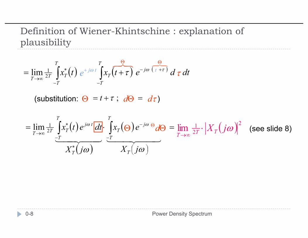
Definition of Wiener-Khintschine : explanation of plausibilityplausibility

( ) ( ) ( ) dtdetxtx jT T

TTτωτ +−∗∫ ∫ += 1lim ttje ω+ τ48476876 ΘΘ

( ) ( ) dtdetxtxT T

TTTTτ

− −∞→ ∫ ∫ +2lim e τ

(substitution: )=+= ;τt τddΘΘ

(see slide 8)( ) 221lim ωjXTTT⋅

∞→( ) ( ) =⋅= −∗

∞→ ∫∫ ωω exdtetx jT

Ttj

T

TTT 21lim ΘΘ Θd

T ∞→

( ) ⎟⎠⎞⎜

⎝⎛

−

∗

−∞→ ∫∫

44 344 214434421ωω jXjX T

T

T

TT

Power Density Spectrum0-8

Response of a linear system to a random input signalResponse of a linear system to a random input signal

impulse response: ( )( )⎩

⎨⎧

tYtX

th:signal output random

:signal input random)(

(Energy-) ACF : ( ) ( ) ( ) ( ) ( )ττττ −∗=+= ∗∞

∞−

∗∫ hhdtththr Ehh

ACF of the output:

CCF f i / t t

( ) ( ) ( ) ( )∗=∗= ττττ XXEhhXXYY rrrr ( ) ( )ττ −∗ ∗hh

( ) ( ) ( )hCCF of in- / output: ( ) ( )∗= ττ XXXY rr ( )τh

PDS of output process: ( ) ( )= ωω jSjS ( ) 2ωjH no phase information!PDS of output process:

Cross-power density spectrum:(between input and output)

( ) ( ) ⋅= ωω jSjS XXYY ( )ωjH

( ) ( ) ⋅= ωω jSjS XXXY ( )ωjH

no phase information!

Response of a Linear System0-9

( p p )

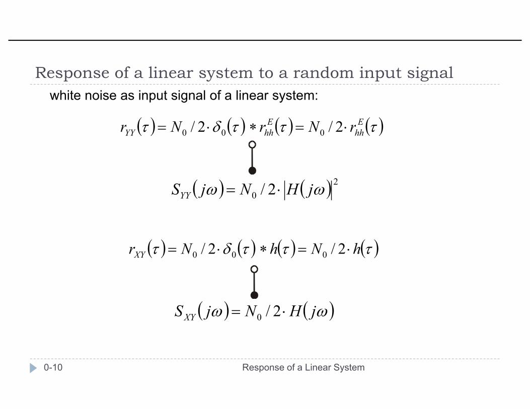
Response of a linear system to a random input signalResponse of a linear system to a random input signalwhite noise as input signal of a linear system:

( ) ( ) ( ) ( )τττδτ EE rNrNr ⋅=∗⋅= 2/2/( ) ( ) ( ) ( )τττδτ hhhhYY rNrNr ⋅=∗⋅= 2/2/ 000

2( ) ( ) 20 2/ ωω jHNjSYY ⋅=

( ) ( ) ( ) ( )τττδτ hNhNrXY ⋅=∗⋅= 2/2/ 000

( ) ( )ωω jHNjSXY ⋅= 2/0

Response of a Linear System0-10