02.09.09 IT 60101: Lecture #15 1

Foundation of Computing Systems

Lecture 15

Searching Algorithms

02.09.09 IT 60101: Lecture #15 2

Searching Techniques

• Several searching techniques

• Linear search– Sequential search with array– Sequential search with linked list– Binary search– Interpolation

– Hashing

• Nonlinear search

– Tree search

» Binary tree search: AVL, Red-black, Splay trees search

– Graph search

» DFS, BFS

02.09.09 IT 60101: Lecture #15 3

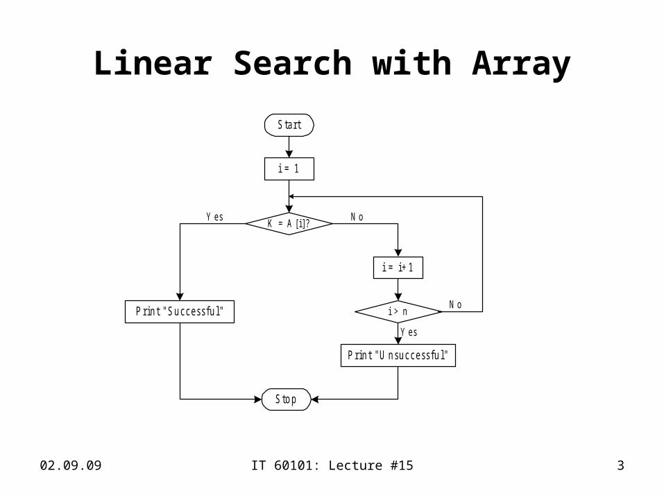
Linear Search with Array

S ta r t

i = 1

K = A [i]?

P r in t " S u c c e s s fu l"

P r in t " U n su c c e ss fu l"

i = i+ 1

i > n

S to p

Y es

Y es

N o

N o

02.09.09 IT 60101: Lecture #15 4

Complexity Analysis: Linear Search

• Case 1: The key matches with the first element• T(n) = 1

• Case 2: Key does not exist• T(n) = n

• Case 3: The key is present at any location in the array

n

ii ipnT

1

)(

npppp ni

121

n

i

in

nT1

1)(

2

1)(

nnT

02.09.09 IT 60101: Lecture #15 5

Complexity Analysis: Summary

2

1)(

nnT

Case Number of key comparisons Asymptotic complexity Remark

Case 1 T(n) = 1 T(n) = O(1) Best case

Case 2 T(n) = n T(n) = O(n) Worst case

Case 3 T(n) = O(n) Average case

02.09.09 IT 60101: Lecture #15 6

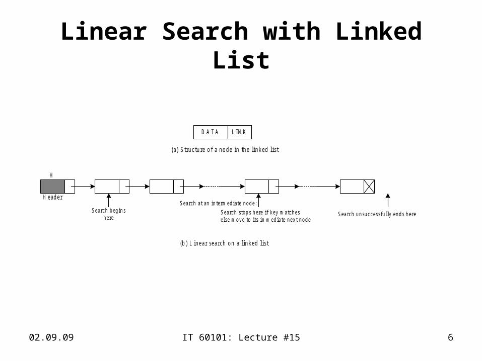
Linear Search with Linked List

D A T A L IN K

(a) S tru c tu re o f a n o d e in th e lin ked lis t

(b ) L in ear search o n a lin ked lis t

H

H ead er

S ea rch b eg in sh ere

S ea rch a t an in term ed ia te n od e:

S ea rch s top s h ere if k ey m atch eselse m ove to its im m ed ia te n ex t n od e

S ea rch u n su ccessfu lly en d s h ere

02.09.09 IT 60101: Lecture #15 7

Complexity Analysis: Linear Search with Linked List

2

1)(

nnT

Case Number of key comparisons Asymptotic complexity Remark

Case 1 T(n) = 1 T(n) = O(1) Best case

Case 2 T(n) = O(n) Average case

Case 3 T(n) = O(n) Worst case2

1)(

nnT

02.09.09 IT 60101: Lecture #15 8

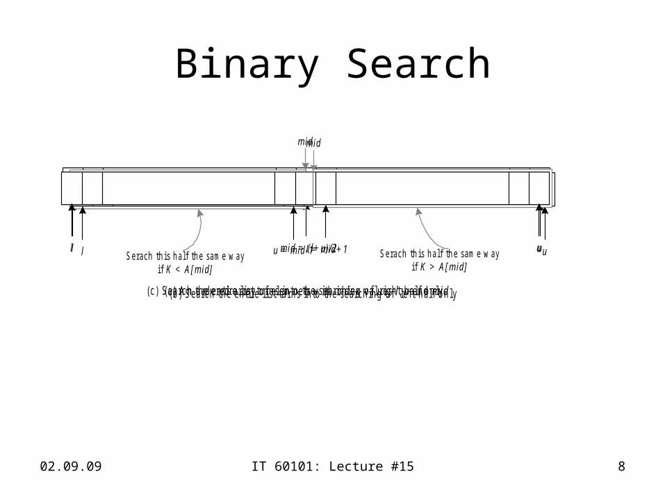
Binary Search

l um id = (l+ u )/2

(a ) A n o rd e re d a r ra y o f e le m n e ts w ith in d e x v a lu e s l , u a n d m id

l u

m id

(b ) S e a rc h th e e n tire lis t tu rn s in to th e se a rc h in g o f le f t-h a lf o n ly

u = m id -1S erach th is h a lf th e sam e w ayif K < A [m id ]

l u

m id

l = m id + 1 S erach th is h a lf th e sam e w ayif K > A [m id ]

(c ) S e a rc h th e e n tire l is t tu rn s in to th e se a rc h in g o f r ig h t-h a lf o n ly

02.09.09 IT 60101: Lecture #15 9

Complexity Analysis of Binary Search

5

F

2 8

9631

74F

F

F

F

F

F

F

F F

<

<

< <

<

<

<

<

<

=

=

= =

=

= =

==

>

> >

>>

> >

> >1 0

F

< = >

02.09.09 IT 60101: Lecture #15 10

Complexity Analysis of Binary Search5

F

2 8

9631

74F

F

F

F

F

F

F

F F

<

<

< <

<

<

<

<

<

=

=

= =

=

= =

==

>

> >

>>

> >

> >1 0

F

< = >

Let n be the total number of elements in the list under search and there exist an integer k such that

• For successful search: – If , then the binary search algorithm requires at least one comparison

and at most k comparisons.

• For unsuccessful search: – If , then the binary search algorithm requires k comparisons.– If , then the binary search algorithm requires either k-1 or k number

of comparisons.

kk n 22 1

12 kn

122 1 kk n

02.09.09 IT 60101: Lecture #15 11

Binary Search: Complexity Analysis

• Best case

T(n) = 1

• Worst case T(n) = 1log2 n

02.09.09 IT 60101: Lecture #15 12

Binary Search: Complexity Analysis

• Average Case– Successful search

– Unsuccessful search

1)( n

InT

1)('

n

EnT

12log

log)( 22

nn

nnnT

1

2log)(' 2

n

nnT

02.09.09 IT 60101: Lecture #15 13

Interpolation Search

02.09.09 IT 60101: Lecture #15 14

Interpolation Search: Complexity Analysis

n

n22 loglog

nn

n

Interpolation search

Successful 1

Unsuccessful

Best case Worst case Average case

02.09.09 IT 60101: Lecture #15 15

Comparison: Successful Search

0

20

40

60

80

100

10 100 500 1000 5000 10000

Input Size

Search array

B inary search

In terpo la tion search

Search lis t

Tim

e (

s)

02.09.09 IT 60101: Lecture #15 16

Comparison: Unsuccessful Search

0

20

40

60

80

100

Input Size

Tim

e (

s)

Search A rray

B inary Search

In terpo la tion search

Search lis t

10 100 500 1000 5000 10000

02.09.09 IT 60101: Lecture #15 17

Nonlinear Search Techniques

A V L T re e se a rc h

N o n lin e a r se a rc h in g

T re e se a rc h G ra p h se a rc h

S p la y tre e se a rc h

R e d -b la c k tre e se a rc h

B in a ry tre e se a rc h D e p th f ir s t s e a rc h

B re d a th f ir s t s e a rc h

02.09.09 IT 60101: Lecture #15 18

Nonlinear Search Techniques: Binary

Search Tree Search

1)1(log2 2 n 1)1(log2 2 n 1)1(log2 2 n

71

14

nH

n 44 1 nH 44 1 nH

Successful search Unsuccessful search

RemarkMinimum number of comparisons

Maximum number of comparisons

Minimum number of comparisons

Maximum number of comparisons

Case 1 1 Best

Case 2 1 2n-1 3 2n+1 Worst

Case 3

1

Average

02.09.09 IT 60101: Lecture #15 19

Graph Search : DFS

1. Push the starting vertex into the stack OPEN

2. While OPEN is not empty do

3. POP a vertex V

4. If V is not in VISIT

5. Visit the vertex V

6. Store V in VISIT

7. Push all the adjacent vertex of V onto OPEN

8. EndIf

9. EndWhile

10. Stop

02.09.09 IT 60101: Lecture #15 20

DFS: Example

v

v

v

v

v

v

v1

2 3

4

5 6

7

v8

v

v

v

v

v

v

v1

2 3

4

5 6

7

v8

D F S

v

v

v

v

v

v

v1

2 3

4

5 6

7

v8

v

v

v

v

v

v

v1

2 3

4

5 6

7

v8

D F S

G 1 G 2

02.09.09 IT 60101: Lecture #15 21

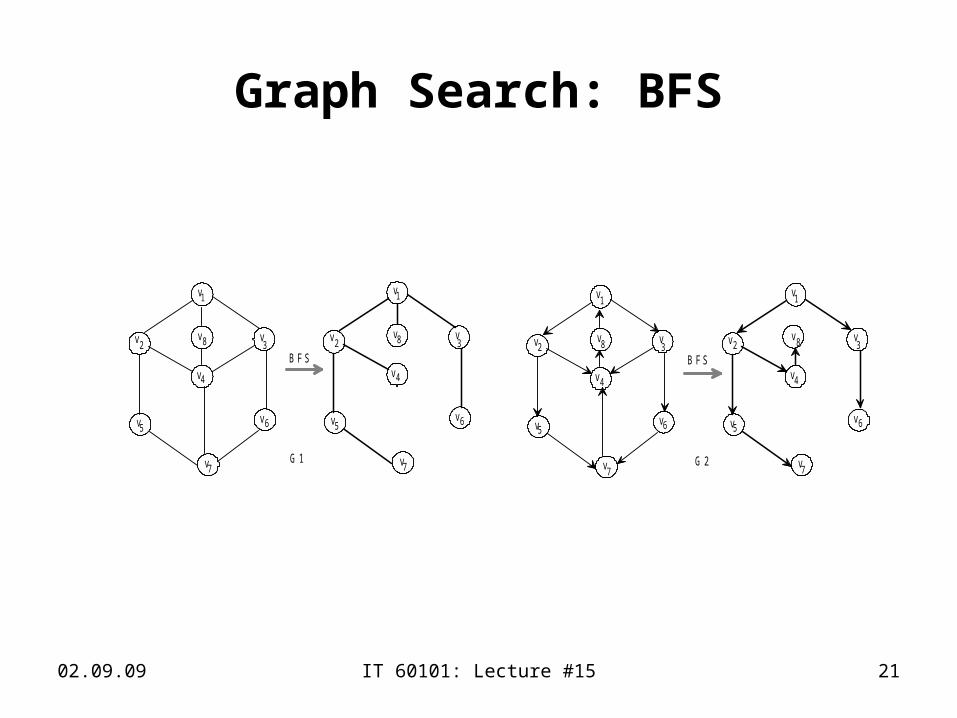
Graph Search: BFS

v

v

v

v

v

v

v1

2 3

4

5 6

7

v8

v

v

v

v

v

v

v1

2 3

4

5 6

7

v8

B F S

G 2

v

v

v

v

v

v

v1

2 3

4

5 6

7

v8

v

v

v

v

v

v

v1

2 3

4

5 6

7

v8

B F S

G 1

02.09.09 IT 60101: Lecture #15 22

Complexity of Graph Search

• T(n) = n.e

• T(n) = n(n-1)

02.09.09 IT 60101: Lecture #15 23

Hashing Techniques

• Address calculation search

1

2

i

m

f(K ) =

K

K...

K

.

.

.

.

.

.

.K

1

2

nA cces tab le

F ile s to rage o fn record s

02.09.09 IT 60101: Lecture #15 24

Hashing Techniques

• Hashing• Is a mappinf from key to its index (location)

.

.

.

.

.

.

.

.

.

.

.

.

.

.

.

.

.

.

.

.

. . .

.

.

.

.

.

.

.. . .

.

.

.

.

.

.

.......

.

.

.

.

.

. . . . .

.........

.

.

.

.

.

.

.

.

.

.

.

.

.

.

.

.

.

.

.

.

.

.

.

.

.

.

.

.

K IH :K I 63 347 734 943 145 986 274 383 501 911 0IK

93 5 , 6 284 373 36

55 9 , 3 1 , 7 744 93

21 011 90

02.09.09 IT 60101: Lecture #15 25

Some Hash Functions

• Division Method

H(k) = k (mod h) if indices starts from 0

H(k) = k (mod h) + 1 if indices start from 1

• Examples

H(31) = 31(mod 13) = 5

H(31) = 31 (mod 13) + 1 = 6

02.09.09 IT 60101: Lecture #15 26

Some Hash Functions

• Midsquare Method

k : 1234 2345 3456

k2: 1522756 5499025 11943936

H(k): 525 492 933

• Limitations• Computationally expensive

02.09.09 IT 60101: Lecture #15 27

Some Hash Functions

• Folding Method

H(k) = k1 + k2 + ... + kn

• Examplek: 1522756 5499025 11943936

Chopping: 01 52 27 56 05 49 90 25 11 94 39 36

Pure folding: 01 + 52 + 27 + 56 05 + 49 + 90 + 25 11 + 94 + 39 + 36

= 136 = 169 = 180

Fold shifting: 10 + 52 + 72 + 56 50 + 49 + 09 + 25 11 + 94 + 93 + 36

= 190 = 133 = 234

Fold boundary: 10 + 52 + 27 + 65 50 + 49 + 90 + 52 11 + 94 + 39 + 63

= 154 = 241 = 207

02.09.09 IT 60101: Lecture #15 28

Collision Resolution Techniques

• Closed hashing – also called linear probing

• Open hashing – also called chaining.

02.09.09 IT 60101: Lecture #15 29

Closed Hashing

• The search will continue until any one of the following cases occurs:

• The key value is found.

• Unoccupied (or empty) location is encountered.

• It reaches to the location where the search was started.

02.09.09 IT 60101: Lecture #15 30

Closed Hashing

• Example• Input: 15  11  25  16  9  8  12  8

• Hash function: H(k) = k mod 7 + 1

1

23456789

1 0

1

23456789

1 0

1

2345

6789

1 0

1

23456789

1 0

1 5 1 5

1 1

1 5

1 12 5

In itia lly th eh a sh ta b le is e m p ty

in se rtio n o f 1 5 in se rtio n o f 1 1 in se rtio n o f 2 5

*

*

*

02.09.09 IT 60101: Lecture #15 31

Closed Hashing

• Example• Input: 15  11  25  16  9  8  12 

• Hash function: H(k) = k mod 7 + 1

1

2345

6789

1 0

1

23456789

1 0

1

2345

6789

1 0

1

2345

6789

1 0

1 5

1 6

1 12 5

1 51 6

91 1

2 5

1 5

1 69

1 12 58

1 51 6

91 12 58

1 2

In se rtio n o f 1 6 In se rtio n o f 9 In se rtio n o f 8

* **

*

In se rtio n o f 1 2

02.09.09 IT 60101: Lecture #15 32

Drawback of Closed Hashing

• Clustering

– key values are clustered in large groups and as a result sequential search becomes slower and slower.

• Following are some solutions known to avoid this situation:

• Random probing

• Double hashing or rehashing

• Quadratic probing

02.09.09 IT 60101: Lecture #15 33

Open Hashing

• Also called separate chaining– This method uses a hash table as an array of pointers– Each pointer points a linked list

• hash table is an array of list headers.

1

23456789

0 1 0

1 2 8 2

4 32 4 6 4 5 4

3 6 1 6

5 7

1 9 3 9

02.09.09 IT 60101: Lecture #15 34

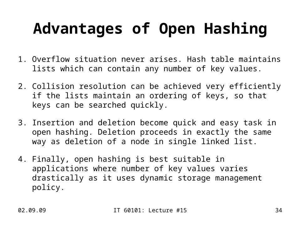
Advantages of Open Hashing

1. Overflow situation never arises. Hash table maintains lists which can contain any number of key values.

2. Collision resolution can be achieved very efficiently if the lists maintain an ordering of keys, so that keys can be searched quickly.

3. Insertion and deletion become quick and easy task in open hashing. Deletion proceeds in exactly the same way as deletion of a node in single linked list.

4. Finally, open hashing is best suitable in applications where number of key values varies drastically as it uses dynamic storage management policy.

02.09.09 IT 60101: Lecture #15 35

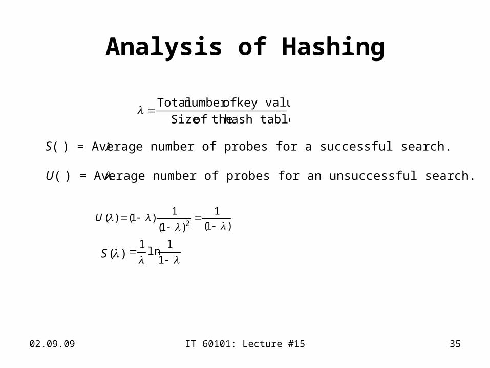
Analysis of Hashing

hash table theof Size

key values ofnumber Total

S( ) = Average number of probes for a successful search.

U( ) = Average number of probes for an unsuccessful search.

)1(

1

)1(

1)1()(

2

U

)(S

1

1ln

1

02.09.09 IT 60101: Lecture #15 36

Analysis of Hashing

)1(

1

)1(

1)1()(

2

U

)(S

1

1ln

1

1

11

2

1)(S

2)1(

11

2

1)(

U

• Closed hashing with random probing

• Close hashing with open probing

• Open hashing

2

1)(

S U

02.09.09 IT 60101: Lecture #15 37

Analysis of Hashing

0 .0

3 .0

6 .0

9 .0

1 2 .0

1 5 .0

1 .0

C lo se d h a sh in g (R a n d o m p ro b in g )C lo se d h a sh in g (L in e a r p ro b in g )O p e n h a sh in g

p , n u m b e r o f p ro b e s

UU (

U ( )

S ( )

S ( )

S ( )

0

0 .0

3 .0

6 .0

9 .0

1 2 .0

1 5 .0

1 .0

C lo se d h a sh in g (R a n d o m p ro b in g )C lo se d h a sh in g (L in e a r p ro b in g )O p e n h a sh in g

p , n u m b e r o f p ro b e s

UU (

U ( )

S ( )

S ( )

S ( )

0

02.09.09 IT 60101: Lecture #15 38

S earch in g

In te ren a l sea rch in g E x te rn a l sea rch in g

L in ear sea rch N o n -lin e ra sea rch

S eq u en tia l sea rch

B in a ry sea rch

In te rp o la tio n sea rch

S earch w ith k ey-co m p ariso n S earch w ith o u t k ey-co m p ariso n

T ree sea rch

B in a ry sea rch tree

R ed -b lack tree sea rch

S p lay tree sea rch

M u lti-w ay tree sea rch

D ig ita l sea rch

G rap h sea rch

A V L tree sea rch

m -w ay tree sea rch

B -tree sea rch

D ep th firs t sea rch

B read th firs t sea rch

A d ress ca lcu la tio n sea rch

B tree sea rch in g

B + tree sea rch in g