Elsner: “02˙ELSNER˙CH02” — 2012/9/24 — 14:22 — page 10 — #1

2R TUTORIAL

“I think it is important for software to avoiding imposing a cognitive style on workers andtheir work.”—Edward Tufte

This chapter is a tutorial on using R. To get the most out of it, you should open an Rsession and type the commands into the console as you read the text. You should beable to use copy-and-paste if you access to an electronic version of the book. All codeis available on the booksWeb site.

2.1 INTRODUCTION

Science requires transparency and reproducibility. TheR language for statisticalmod-eling makes this easy. Developing, maintaining, and documenting your R code issimple. R contains numerous functions for organizing, graphing, and modeling yourdata. Directions for obtaining R, accompanying packages, and other sources of docu-mentation are available athttp://www.r-project.org/. Anyone serious aboutapplying statistics to climate data should learn R.The book is self-contained. It presents R code and data (or links to data) that can be

copied and pasted to reproduce the graphs and tables. This reproducibility providesyouwith an enhanced learning opportunity.Here we present a tutorial to help you getstarted. This can be skipped if you already know how to work with R.

2.1.1 What Is R?

R is the ‘lingua franca’ of data analysis and statistical computing. It helps you performa variety of computing tasks by giving you access to commands. This is similar toother programming languages such as Python and C++. R is particularly useful to

10

Elsner: “02˙ELSNER˙CH02” — 2012/9/24 — 14:22 — page 11 — #2

11 Introduction

researchers because it contains a number of built-in mechanisms for organizing data,performing calculations, and creating graphics.R is an open-source statistical environment modeled after S. The S language was

developed in the late 1980s at AT&T labs. The R project was started by Robert Gen-tleman and Ross Ihaka of the Statistics Department of the University of Aucklandin 1995. It now has a large audience. It is currently maintained by the R core-development team, an international group of volunteer developers. To get to the Rproject Web site, open a browser and, in the search window, type the keywords “Rproject” or directly link to the Web page using http://www.r-project.org/.Directions for obtaining the software, accompanying packages, and other sources ofdocumentation are provided at the site.Why use R? It is open source, free, runs on the major computing platforms, has

built-in help and excellent graphing capabilities, and it is powerful, extensible, andcontains thousands of functions. A drawback to R for many is the lack of a seriousgraphical user interface (GUI). This means that it is harder to learn at the outsetand you need to appreciate syntax. Modern ways of working with computers includebrowsers, music players, and spreadsheets. R is nothing like these. Infrequent usersforget commands. There are no visual cues; a blank screen is intimidating. At first,working with R might seem daunting. However, with a little effort, you will quicklylearn the basic commands and then realize how it can help you do much, much more.R is really a library of modern statistical tools. It is unmatched in its breadth and

scope. A climate scientist whose research requires customized scripting, extensivesimulation analysis, or state-of-the-art statistical analysis will find R to be a solid foun-dation. R is also a language. It has rules and syntax. R can be run interactively, andanalysis can be done on the fly. It is not limited by a finite set of functions. You candownload packages to perform specialized analysis and graph the results. R is objectoriented, allowing you to define new objects and create your own methods for them.Many people use spreadsheets. This is good for tasks such as data storage and

manipulation. Unfortunately, spreadsheets are unsuitable for serious research. This isbecause it is hard tomake publication-quality graphs, there is limited community sup-port for newmethods, and it can be a challenge to share your calculations with others.If you are serious about reproducible research, you should not use a spreadsheet forstatistics.

2.1.2 Get R

At the R project Web site, click on CRAN (Comprehensive R Archive Network) andselect a nearby mirror site. Then follow instructions appropriate for your operatingsystem to download the base distribution. On your computer, click on the downloadicon and follow the install instructions. Click on the icon to start R. If you are usingthe Linux operating system, type the letter R from a command window.R ismost easily used in an interactivemanner.You ask R a question and it gives you

an answer. Questions are asked and answered on the command line. The > (greaterthan symbol) is used as the prompt. Throughout this book, it is the character that is

Elsner: “02˙ELSNER˙CH02” — 2012/9/24 — 14:22 — page 12 — #3

12 R Tutorial

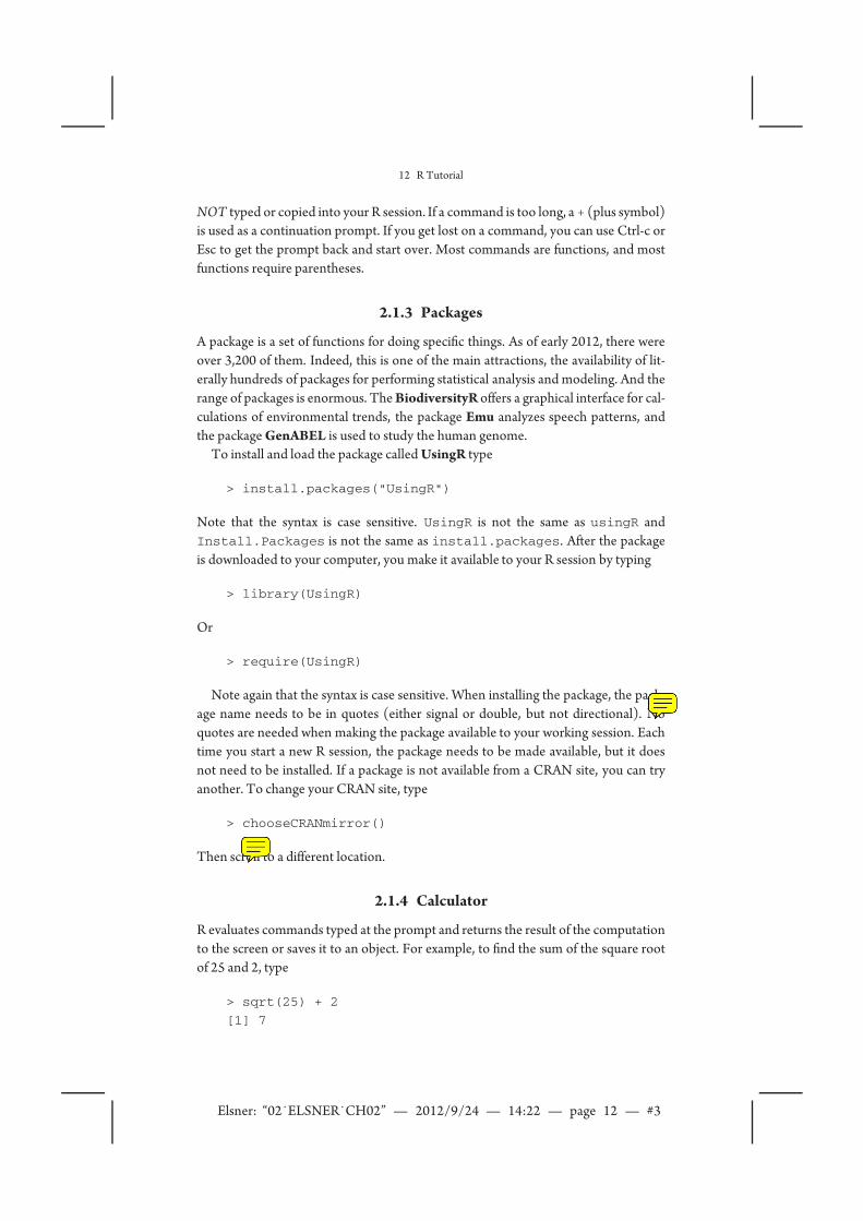
NOT typed or copied into your R session. If a command is too long, a + (plus symbol)is used as a continuation prompt. If you get lost on a command, you can use Ctrl-c orEsc to get the prompt back and start over. Most commands are functions, and mostfunctions require parentheses.

2.1.3 Packages

A package is a set of functions for doing specific things. As of early 2012, there wereover 3,200 of them. Indeed, this is one of the main attractions, the availability of lit-erally hundreds of packages for performing statistical analysis and modeling. And therange of packages is enormous. TheBiodiversityR offers a graphical interface for cal-culations of environmental trends, the package Emu analyzes speech patterns, andthe packageGenABEL is used to study the human genome.To install and load the package calledUsingR type

> install.packages("UsingR")

Note that the syntax is case sensitive. UsingR is not the same as usingR andInstall.Packages is not the same as install.packages. After the packageis downloaded to your computer, you make it available to your R session by typing

> library(UsingR)

Or

> require(UsingR)

Note again that the syntax is case sensitive. When installing the package, the pack-age name needs to be in quotes (either signal or double, but not directional). Noquotes are needed when making the package available to your working session. Eachtime you start a new R session, the package needs to be made available, but it doesnot need to be installed. If a package is not available from a CRAN site, you can tryanother. To change your CRAN site, type

> chooseCRANmirror()

Then scroll to a different location.

2.1.4 Calculator

R evaluates commands typed at the prompt and returns the result of the computationto the screen or saves it to an object. For example, to find the sum of the square rootof 25 and 2, type

> sqrt(25) + 2

[1] 7

Elsner: “02˙ELSNER˙CH02” — 2012/9/24 — 14:22 — page 13 — #4

13 Introduction

The [1] says “first requested element will follow.” Here there is only one element,the answer 7. The > prompt that follows indicates R is ready for another command.For example, type

> 12/3 - 5

[1] -1

R uses order of operations so that, for instance, multiplication comes before addition.How would you calculate the 5th power of 2? Type

> 2ˆ5

[1] 32

How about the amount of interest on $1,000, compounded annually at 4.5 percent(annual percentage) for 5 years? Type

> 1000 * (1 + .045)ˆ5 - 1000

[1] 246

2.1.5 Functions

There are numerousmathematical and statistical functions available in R. They are allused in a similar manner. A function has a name, which is typed, followed by a pair ofparentheses (required). Arguments are added inside the parentheses as needed. Forexample, the square root of two is given as

> sqrt(2) # the square root

[1] 1.41

The # is the comment character. Any text in the line following this character is treatedas a comment and is not evaluated. Some other examples include

> sin(pi) # the sine function

[1] 1.22e-16

> log(42) # log of 42 base e

[1] 3.74

Most functions have arguments that allow you to change the default behavior. Forexample, to use base 10 for the logarithm, you can use either of the following:

> log(42, 10)

[1] 1.62

> log(42, base=10)

[1] 1.62

To understand the first function, log(42,10), you need to know that R expects thebase to be the second argument (after the first comma) of the function. The secondexample uses a named argument of the type base=10 to explicitly set the base value.

Elsner: “02˙ELSNER˙CH02” — 2012/9/24 — 14:22 — page 14 — #5

14 R Tutorial

The first style contains less typing, but the second style is easier to remember andgood coding practice.

2.1.6 Warnings and Errors

When R does not understand your function, it responds with an error message. Forexample

> srt(2)

Error in try(srt(2)) : could not find function "srt"

If you get the function correct, but your input is not acceptable, then

> sqrt(-2)

NaN

The output NaN is used to indicate “not a number.”As mentioned, if R encounters a line that is not complete, a continuation prompt,

+, is printed, indicating more input is expected. You can complete the line after thecontinuation prompt.

2.1.7 Assignments

It is convenient to name an object so that you can use it later. Doing so is called anassignment. Assignments are straightforward. You put a name on the left-hand side ofthe equals sign and a value, function, object, and so on, on the right. Assignments donot usually produce printed output.

> x = 2 # assignments return a prompt only

> x + 3 # x is now 2

[1] 5

Remember, the pound symbol (#) is used as a comment character. Anything after the# is ignored. Adding comments to your code is a way of recalling what you did andwhy.You are free tomake object names out of letters, numbers, and the dot or underline

characters. A name starts with a letter or a dot (a leading dot may not be followed by anumber). You are not allowed to use math operators, such as +, -, *, and /. The helppage for make.names describes this in more detail (?make.names).Note that case is also important in names; x is different than X. It is good practice

to use conventional names for data types. For instance, n is for the number of datarecords or the length of a vector, x and y are used for spatial coordinates, and i and jare used for integers and indices for vectors and matrices. These conventions are notforced, but consistency makes it easier for others to understand your code.

Elsner: “02˙ELSNER˙CH02” — 2012/9/24 — 14:22 — page 15 — #6

15 Data

Variables that beginwith the dot character are reserved for advanced programmers.Unlike many programming languages, the period in R is used only as a punctuationand can be included in an object name (e.g., my.object).

2.1.8 Help

Using R to do statistics requires knowing many functions—more than you can likelykeep in your head. R has built-in help for information about what is returned by thefunction, for details on additional arguments, and for examples. If you know the nameof a function, type

> help(var)

This brings up a help page for the function named inside the parentheses. (?varworks the same way). The name of the function and the associate package is givenas the help page preamble. This is followed by a brief description of the function andhow it is used. Arguments are explained along with function and argument details.Examples are given toward the bottom of the page. A good way to understand what afunction does is to run the examples.Most help pages provide examples. The examples help you understand what the

function does. You can try the examples individually by copying and pasting theminto your R session. You can also try them all at once by using the example function.For instance, type

> example(mean)

Help pages work great if you know the name of the function. If not, the func-tion help.search("mean") searches each entry in the help system and returnsmatches (often many) of functions that mention the word "mean". The functionapropos searches through only function names and variables for matches. Type

> apropos("mean")

To end your R session, type

> q(save="no")

Like most R functions, q needs an open (left) and close (right) parentheses. Theargumentsave="no" says do not save the workspace. Otherwise the workspace andsession history are saved to a file in your working directory.By default, the file is called.RData. Theworkspace is your current Rworking environment and includes all yourobjects, including vectors, matrices, data frames, lists, functions and so on.

2.2 DATA

2.2.1 Small Amounts

To begin, you need to get your data into R. For small amounts, you use the c func-tion, which combines (concatenates) items. Consider a set of hypothetical hurricane

Elsner: “02˙ELSNER˙CH02” — 2012/9/24 — 14:22 — page 16 — #7

16 R Tutorial

counts, where in the first year there were two landfalls, in the second there were three,landfalls and so on. To enter these values, type

> h = c(2, 3, 0, 3, 1, 0, 0, 1, 2, 1)

The 10 values are stored in a vector object of class numeric called h.

> class(h)

[1] "numeric"

To show the values, type the name of the object.

> h

[1] 2 3 0 3 1 0 0 1 2 1

Take note. You assigned the values to an object called h. The assignment operator isan equal sign (=). Another assignment operator used frequently is <-, a left-pointingarrow that consists of two keystrokes (the less-than sign and the hyphen). This isthe more common of the assignment operators. The equal sign is used in declaringargument values, so confusion can arise if it is also used as the assignment operator.With most assignments, only the prompt is returned to the screen with nothing

printed. The object to the left of the assignment operator is given the values of what-ever is to the right of the operator. Objects are printed by typing the object name asyou just did. Finally, the values when printed are prefaced with a [1]. This indicatesthat the first entry in the object has a value of 2 (the number immediately to the rightof [1]). More on this later.The arrow keys can be used to retrieve previous functions. This saves typing. Each

command is stored in a history file and the up arrow key moves backward through thehistory file and the down arrowmoves forward. The left and right arrow keys work asexpected. Changes can be made to a mistyped function followed by a return withoutthe need to go to the end of the line.You can also enter small amounts of data with the scan function. You enter data

values one at a time line by line. When finished, type enter (return). R has a widerange of functions for inputting data. We will look at them as needed.

2.2.2 Functions

Once the data are stored as an object, you call functions to do various things. Forexample, you find the total number of landfalls occurring over the set of years bytyping

> sum(h)

[1] 13

The function adds up the values of the vector elements.The number of years is found by typing

> length(h)

[1] 10

Elsner: “02˙ELSNER˙CH02” — 2012/9/24 — 14:22 — page 17 — #8

17 Data

The average number of hurricanes over this 10 year period is found by typing

> sum(h)/length(h)

[1] 1.3

or

> mean(h)

[1] 1.3

Other useful functions include sort, min, max, range, diff, and cumsum.Try them on the object h of landfall counts. For example, what does the functiondiff do?Most functions have a name followed by a left parenthesis, then a set of arguments

separated by commas followed by a right parenthesis. Arguments have names. Someare required, but many are optional with R providing default values. Throughoutthis book, function name references in line are left without arguments and withoutparentheses.In summary, consider the code

> x = log(42, base=10)

Here x is the object name, = is the assignment operator,log is the function, 42 is thevalue for which the logarithm is being computed, and 10 is the argument correspond-ing to the logarithm base. Note here the equal sign is used in two different ways: as anassignment operator and to specify a value for an argument.

2.2.3 Vectors

Your earlier data object h from previously is stored as a vector. This means that Rkeeps track of the order you entered the data. The vector contains a first element, asecond element, and so on. This is convenient.Your data of landfall counts has a natural order—year 1, year 2, and so on—so you

want to keep this order. You would like to be able to make changes to the data itemby item instead of reentering the entire data. R lets you do this. Also vectors are mathobjects so math operations can be performed on them.Let us see how these concepts apply to your data. Suppose h contains the annual

landfall counts from the first decade of a longer record. You want to keep track ofcounts over a second decade. This can be done as follows:

> d1 = h # make a copy

> d2 = c(0, 5, 4, 2, 3, 0, 3, 3, 2, 1)

Most functions will operate on each vector component (element) all at once.

> d1 + d2

[1] 2 8 4 5 4 0 3 4 4 2

> d1 - d2

Elsner: “02˙ELSNER˙CH02” — 2012/9/24 — 14:22 — page 18 — #9

18 R Tutorial

[1] 2 -2 -4 1 -2 0 -3 -2 0 0

> d1 - mean(d1)

[1] 0.7 1.7 -1.3 1.7 -0.3 -1.3 -1.3 -0.3 0.7

[10] -0.3

In the first two cases, the first-year count of the first decade is added (and subtracted)from the first-year count of the second decade and so on. In the third case, a constant(the average of the first decade) is subtracted from each count of the first decade.Thisis an example of recycling. R repeats values from one vector so as to match the lengthof the other vector. Here the mean value is computed and then repeated 10 times.The subtraction then follows on each component one at a time.Suppose you are interested in the variability of hurricane counts from one year to

the next. An estimate of this variability is the variance. The sample mean of a set ofnumbers y is

y=1n

n

∑i=1

yi, (2.1)

where n is the sample size. And the sample variance is

s2 =1

n− 1

n

∑i=1

(yi − y)2. (2.2)

Although the function var will compute the sample variance, to see how vector-ization works in R, you write few lines of code.

> dbar = mean(d1)

> dif = d1 - dbar

> ss = sum(difˆ2)

> n = length(d1)

> ss/(n - 1)

[1] 1.34

Note how the different parts of the equation for the variance (2.2) match what youtype in R. To verify your code, type

> var(d1)

[1] 1.344444

To change the number of significant digits printed to the screen from the default of7, type

> options(digits=3)

> var(d1)

[1] 1.34

Elsner: “02˙ELSNER˙CH02” — 2012/9/24 — 14:22 — page 19 — #10

19 Data

The standard deviation, which is the square root of the variance, is obtained bytyping

> sd(d1)

[1] 1.16

One restriction on vectors is that all the components must have the same type.You cannot create a vector with the first component a numeric value and the secondcomponent a character text. A character vector can be a set of text strings as in

> Elsners = c("Jim", "Svetla", "Ian", "Diana")

> Elsners

[1] "Jim" "Svetla" "Ian" "Diana"

Note that character strings are made by matching quotes on both sides of the string,either double, "", or single, '. Caution: The quotes must not be directional. If youcopy your code from a word processor (such as MS Word) the program will insertdirectional quotes. It is better to copy from a text editor such as Notepad.You add another component to the vector Elsners by using the c function.

> c(Elsners, 1.5)

[1] "Jim" "Svetla" "Ian" "Diana" "1.5"

The component 1.5 gets coerced to a character string. Coercion occurs for mixedtypeswhere the components get changed to the lowest common type, which is usuallya character. You cannot perform arithmetic on a character vector.Elements of a vector can have names. The names will appear when you print the

vector. You use the names function to retrieve and set names as character strings. Forinstance, you type

> names(Elsners) = c("Dad", "Mom", "Son", "Daughter")

> Elsners

Dad Mom Son Daughter

"Jim" "Svetla" "Ian" "Diana"

Unlike most functions, names appears on the left side of the assignment operator.The function adds the names attribute to the vector. Names can be used on vectors ofany type.Returning to your hurricane example, suppose the National Hurricane Center

(NHC) finds a previously undocumented hurricane in the sixth year of the seconddecade. In this case, you type

> d2[6] = 1

This changes the sixth element (component) of vectord2 to 1, leaving the other com-ponents alone. Note the use of square brackets ([]). Square brackets are used tosubset components of vectors (and arrays, lists, etc.), whereas parentheses are usedwith functions to enclose the set of arguments.

Elsner: “02˙ELSNER˙CH02” — 2012/9/24 — 14:22 — page 20 — #11

20 R Tutorial

You list all values in vector d2 by typing

> d2

[1] 0 5 4 2 3 1 3 3 2 1

To print the number of hurricanes during the third year only, type

> d2[3]

[1] 4

To print all the hurricane counts except from the fourth year, type

> d2[-4]

[1] 0 5 4 3 1 3 3 2 1

To print the hurricane counts for the odd years only, type

> d2[c(1, 3, 5, 7, 9)]

[1] 0 4 3 3 2

Here you use the c function inside the subset operator [.Since here you want a regular sequence of years, the expression c(1,3,5,7,9)

can be simplified using structured data.

2.2.4 StructuredData

Sometimes a set of values has a pattern. The integers from 1 through 10, for example.To enter these one by one using the c function is tedious. Instead, the colon functionis used to create sequences. For example, to sequence the first 10 positive integers,you type

> 1:10

[1] 1 2 3 4 5 6 7 8 9 10

Or to reverse the sequence, you type

> 10:1

[1] 10 9 8 7 6 5 4 3 2 1

You create the same reversed sequence of integers using the rev function togetherwith the colon function as

> rev(1:10)

The seq function is more general than the colon function. It allows for not onlystart and end values, but also a step size or sequence length. Some examples include

> seq(1, 9, by=2)

[1] 1 3 5 7 9

> seq(1, 10, by=2)

[1] 1 3 5 7 9

Elsner: “02˙ELSNER˙CH02” — 2012/9/24 — 14:22 — page 21 — #12

21 Data

> seq(1, 9, length=5)

[1] 1 3 5 7 9

Use the rep function to create a vector with elements having repeat values. Thesimplest usage of the function is to replicate the value of the first argument the numberof times specified by the value of the second argument.

> rep(1, times=10)

[1] 1 1 1 1 1 1 1 1 1 1

or

> rep(1:3, times=3)

[1] 1 2 3 1 2 3 1 2 3

You create more complicated patterns by specifying pairs of equal-sized vectors. Inthis case, each component of the first vector is replicated the corresponding numberof times as specified in the second vector.

> rep(c("cold", "warm"), c(1, 2))

[1] "cold" "warm" "warm"

Here the vectors are implicitly defined using the c function and the name of the sec-ond argument (times) is left off. Again it is good coding practice to name thearguments. If you name the arguments, then the order in which they appear in thefunction is not important.Suppose you want to repeat the sequence of cold, warm, warm three times. You

nest the above sequence generator in another repeat function as follows:

> rep(rep(c("cold", "warm"), c(1, 2)), 3)

[1] "cold" "warm" "warm" "cold" "warm" "warm" "cold" [8]

"warm" "warm"

Function nesting gives you a lot of flexibility.

2.2.5 Logic

As you have seen, there are functions like mean andvar that when applied to a vectorof data output a statistic. Another example is the max function. To find the maximumnumber of hurricanes in a single year during the first decade, type

> max(d1)

[1] 3

This tells you that the worst year had three hurricanes.To determine which years had this many hurricanes, type

> d1 == 3

[1] FALSE TRUE FALSE TRUE FALSE FALSE FALSE FALSE

[9] FALSE FALSE

Elsner: “02˙ELSNER˙CH02” — 2012/9/24 — 14:22 — page 22 — #13

22 R Tutorial

Note the double equal sign. Recall a single equal sign assigns d1 the value 3. With thedouble equal sign you are performing a logical operation on the components of thevector. Each component is matched in value with the value 3, and a true or false isreturned. That is, is component one equal to 3? No, so return FALSE; is componenttwo equal to 3? Yes, so return TRUE, and so on. The length of the output will matchthe length of the vector.Now how can you get the years corresponding to the TRUE values? To rephrase,

which years have three hurricanes? If you guessed the function which, you are onyour way to mastering R.

> which(d1 == 3)

[1] 2 4

You might be interested in the number of years in each decade without ahurricane.

> sum(d1 == 0); sum(d2 == 0)

[1] 3

[1] 1

Here we apply two functions on a single line by separating the functions with asemicolon.Or how about the ratio of the number of hurricanes over the two decades.

> mean(d2)/mean(d1)

[1] 1.85

So there is 85 percent more landfalls during the second decade. The statisticalquestion is, is this difference significant?Before moving on, it is recommended that you remove objects from your

workspace that are no longer needed. This helps you recycle names and keeps yourworkspace clean. First, to see what objects reside in your workspace, type

> objects()

[1] "Elsners" "RweaveLatex2"

[3] "RweaveLatexRuncode2" "Sweave2"

[5] "d1" "d2"

[7] "dbar" "dif"

[9] "h" "n"

[11] "ss" "tikz.Swd"

[13] "try_out" "x"

Then, to remove only selected objects, type

> rm(d1, d2, Elsners)

To remove all objects, type

> rm(list=objects())

Elsner: “02˙ELSNER˙CH02” — 2012/9/24 — 14:22 — page 23 — #14

23 Data

Thiswill clean your workspace completely. To avoid name conflicts it is good practiceto start a session with a clean workspace. However do not include this command incode you give to others.

2.2.6 Imports

Most of what you do in R involves data. To get data into R, first you need to knowyour working directory. You do this with the getwd function by typing

> getwd()

[1] "/Users/jelsner/Dropbox/book/Chap02"

The output is a character string in quotes that indicates the full path of your workingdirectory on your computer. It is the directory where R will look for data. To changeyour working directory, you use thesetwd function and specify the path namewithinquotes. Alternatively, you should be able to use one of the menu options in the R,console. To list the files in your working directory, you type dir().Second, you need to know the file type of your data. This will determine the read

function. For example, the data setUS.txt contains a list of tropical cyclone counts byyear making landfall in the United States (excluding Hawaii) at hurricane intensity.The file is a space-delimited text file. In this case, you use the read.table functionto import the data.Third, you need to knowwhether your data file has column names. These are given

in the first line of your file, usually as a series of character strings. The line is called a“header”, and if your data have one, you need to specify header=TRUE.Assuming the text fileUS.txt is in your working directory, type

> H = read.table("US.txt", header=TRUE)

If R returns a prompt without an error message, the data have been imported. Hereyour file contains a header so the argument header is used.At this stage, the most common mistake is that your data file is not in your work-

ing directory. This will result in an error message along the lines of “cannot open theconnection” or “cannot open file.”The function has options for specifying the separator character or characters

between columns in the file. For example, if your file has commas between columns,then you use the argument sep="," in the read.table function. If the file hastabs, then you use sep="\t". Note that R makes no changes to your original file.You can also change the missing value character. By default, it is NA. If the missing

value character in your file is coded as 99, specify na.strings="99", and it will bechanged to NA in your R data object.There are several variants of read.table that differ only in the default argument

settings. Note in particularread.csv, which has settings that are suitable for commadelimited (csv) files that have been exported from a spreadsheet. Thus, the typicalwork flow is to export your data from a spreadsheet to a csv file, then import it to Rusing the read.csv function.

Elsner: “02˙ELSNER˙CH02” — 2012/9/24 — 14:22 — page 24 — #15

24 R Tutorial

You can also import data directly from the web by specifying the URL instead ofthe local file name.

> loc = "http://myweb.fsu.edu/jelsner/US.txt"

> H = read.table(loc, header=TRUE)

The object H is a data frame and the function read.table and variants returndata frames. Data frames are similar to a spreadsheet. The data are arranged in rowsand columns. The rows are the cases and the columns are the variables. To check thedimensions of your data frame, type

> dim(H)

[1] 160 6

This tells you that there are 160 rows and 6 columns in your data frame.To list the first six lines of the data object, type

> head(H)

Year All MUS G FL E

1 1851 1 1 0 1 0

2 1852 3 1 1 2 0

3 1853 0 0 0 0 0

4 1854 2 1 1 0 1

5 1855 1 1 1 0 0

6 1856 2 1 1 1 0

The columns include year, number of U.S. hurricanes, number of major U.S. hur-ricanes, number of U.S. Gulf coast hurricanes, number of Florida hurricanes, andnumber of East coast hurricanes in order. Note that the column names are given aswell. The last six lines of your data frame are listed similarly using the tail function.The number of lines listed is changed using the argument n (for example, n=3).If your data reside in a directory other than your working directory, you can use

the file.choose function. This will open a dialog box allowing you to scrolland choose the file. Note that the default for this function has no arguments:file.choose().Tomake the individual columns available by column name, type

> attach(H)

All, E, FL, G, MUS, Year

The total number of years in the record is obtained and saved in n, and the averagenumber of U.S. hurricanes is saved in rate using the following two lines of code:

> n = length(All)

> rate = mean(All)

By typing the names of the saved objects, the values are printed.

> n

[1] 160

Elsner: “02˙ELSNER˙CH02” — 2012/9/24 — 14:22 — page 25 — #16

25 Tables and Plots

> rate

[1] 1.69

Thus over the 160 years of data, the average number of U.S. hurricanes per year is1.69.If you want to change the names of the data frame, type

> names(H)[4] = "GC"

> names(H)

[1] "Year" "All" "MUS" "GC" "FL" "E"

This changes the fourth column name from G to GC. Note that this is done to thedata frame in R and not to your original data file.While attaching a data frame is convenient, it is not a good strategy when writing

R code as name conflicts can easily arise. If you do attach your data frame, make sureyou use the function detach after you are finished.

2.3 TABLES AND PLOTS

Now that you know a bit about using R, you are ready for some data analysis. R hasa wide variety of data structures including scalars, vectors, matrices, data frames, andlists.

2.3.1 Tables and Summaries

Vectors and matrices must have a single class. For example, the vectors A, B, and Cbelow are constructed as numeric, logical, and character respectively.

> A = c(1, 2.2, 3.6, -2.8) #numeric vector

> B = c(TRUE, TRUE, FALSE, TRUE) #logical vector

> C = c("Cat 1", "Cat 2", "Cat 3") #character vector

To view the data class, type

> class(A); class(B); class(C)

[1] "numeric"

[1] "logical"

[1] "character"

Let the vector wx denote the weather conditions for five forecast periods ascharacter data.

> wx = c("sunny", "clear", "cloudy", "cloudy", "rain")

> class(wx)

[1] "character"

Elsner: “02˙ELSNER˙CH02” — 2012/9/24 — 14:22 — page 26 — #17

26 R Tutorial

Character data are summarized using thetable function. To summarize theweatherconditions over the 6 days, type

> table(wx)

wx

clear cloudy rain sunny

1 2 1 1

The output is a list of the unique character strings and the corresponding number ofoccurrences of each string.As another example, let the object ss denote the Saffir–Simpson category for a set

of five hurricanes.

> ss = c("Cat 3", "Cat 2", "Cat 1", "Cat 3", "Cat 3")

> table(ss)

ss Cat 1 Cat 2 Cat 3

1 1 3

Here the character strings correspond to intensity levels as ordered categories withCat 1 < Cat 2 < Cat 3. In this case, it is better to convert the character vectorss to an ordered factor with levels. This is done using the factor function.

> ss = factor(ss, order=TRUE)

> class(ss)

[1] "ordered" "factor"

> ss

[1] Cat 3 Cat 2 Cat 1 Cat 3 Cat 3

Levels: Cat 1 < Cat 2 < Cat 3

The class of ss gets changed to an ordered factor. A print of the object results in a listof the elements in the vector and a list of the levels in order. Note, if you do the samefor the wx object, the order is alphabetical by default. Try it.You can also use the table function on discrete numeric data. For example,

> table(All)

All

0 1 2 3 4 5 6 7

34 48 38 27 6 1 5 1

The table tells you that your data has 34 zeros, 48 ones, and so on. Since these areannual U.S. hurricane counts, you know, for instance, that there are 6 years with fourhurricanes and so on.Recall from the previous section that you attached the data frame H so you can use

the column names as separate vectors. The data frame remains attached for the entiresession. Remember that you detach it with the function detach.The summary function is used to a get a description of your object. The form of the

value(s) returned depends on the class of the object being summarized. If your objectis a data frame of the summary consisting of numeric data the output are six summary

Elsner: “02˙ELSNER˙CH02” — 2012/9/24 — 14:22 — page 27 — #18

27 Tables and Plots

statistics (mean, median, minimum, maximum, first quartile, and third quartile) foreach column.

> summary(H)

Year All MUS

Min. :1851 Min. :0.00 Min. :0.0

1st Qu.:1891 1st Qu.:1.00 1st Qu.:0.0

Median :1930 Median :1.00 Median :0.0

Mean :1930 Mean :1.69 Mean :0.6

3rd Qu.:1970 3rd Qu.:2.25 3rd Qu.:1.0

Max. :2010 Max. :7.00 Max. :4.0

GC FL E

Min. :0.000 Min. :0.000 Min. :0.000

1st Qu.:0.000 1st Qu.:0.000 1st Qu.:0.000

Median :0.500 Median :0.000 Median :0.000

Mean :0.688 Mean :0.681 Mean :0.469

3rd Qu.:1.000 3rd Qu.:1.000 3rd Qu.:1.000

Max. :4.000 Max. :4.000 Max. :3.000

Each column of your data frame H is labeled and summarized by six numbers includ-ing theminimum, themaximum, themean, themedian, and the first (lower) and third(upper) quartiles. For example, you see that the maximum number of major U.S. hur-ricanes (MUS) in a single season is 4. Since the first column is the year, the summary isnot particularly meaningful.

2.3.2 Quantiles

The quartiles from the summary function are examples of quantiles. Sample quan-tiles cut a set of ordered data into equal-sized data bins. The ordering comes fromrearranging the data from lowest to highest. The first, or lower, quartile correspond-ing to the .25 quantile (25th percentile) indicates that 25 percent of the data have avalue less than this quartile value. The third, or upper, quartile corresponding to the.75 quantile (75th percentile) indicates that 75 percent of the data have a smaller valuethan this quartile value.The quantile function calculates sample quantiles on a vector of data. For exam-

ple, consider the set of North Atlantic Oscillation (NAO) index values for the monthof June from the period 1851 to 2010. The NAO is a variation in the climate over theNorthAtlanticOcean, featuring fluctuations in the difference of atmospheric pressureat sea level between the Iceland and the Azores. The index is computed as the differ-ence in standardized sea-level pressures. The standardization is done by subtractingthe mean and dividing by the standard deviation. The units on the index is standarddeviation. See Chapter 6 for more details on these data.First read the data consisting of monthly NAO values, then apply the quantile

function to the June values.

Elsner: “02˙ELSNER˙CH02” — 2012/9/24 — 14:22 — page 28 — #19

28 R Tutorial

> NAO = read.table("NAO.txt", header=TRUE)

> quantile(NAO$Jun, probs=c(.25, .5))

25% 50%

-1.405 -0.325

Note the use of the $ sign to point to a particular column in the data frame. Recall thatto list the column names of the data frame object called NAO, type names(NAO).Of the 160 values, 25 percent of them are less than -1.4 standard deviations (s.d.),

50 percent are less than -0.32 s.d. Thus there are an equal number of years with JuneNAO values between -1.4 and -0.32 s.d.The third quartile value corresponding to the .75 quantile (75th percentile) indi-

cates that 75% of the data have a value less than this. The difference between the firstand third quartile values is called the interquartile range (IQR). Fifty percent of allvalues lie within the IQR. The IQR of a data vector can be found by using the IQRfunction.

2.3.3 Plots

R has a wide range of plotting capabilities. It takes time to master, but a little effortgoes a long way. You will create a lot of plots as you work through this book. Here area few examples to get you started. Chapter 5 provides more details.

Bar Plots

The bar plot (or bar chart) is a way to compare categorical or discrete data. Levels ofthe variable are arranged in some order along the horizontal axis and the frequencyof values in each group is plotted as a bar with the bar height proportional to thefrequency.Tomake a bar plot of your U.S. hurricane counts, type

> barplot(table(All), ylab="Number of Years",

+ xlab="Number of Hurricanes")

The plot in Figure 2.1 is a concise summary of the number of hurricanes. The barheights are proportional to the number years with that many hurricanes. The plotconveys the same information as the table. The purpose of the bar plot is to illustratethe difference between data values. Readers expect the plot to start at zero, so youshould try to draw it that way. Also usually there is little scientific reason to make thebars appear three dimensional.Note that the axis labels are set using the ylab and xlab arguments with the label

as a character string in quotation. R careful to avoid the directional quotes that appearin word-processing type.Althoughmany of the plotting commands are simple and somewhat intuitive, to get

a publication-quality figure requires tweaking the default settings. You will see someof these tweaks as you work through the book.

Elsner: “02˙ELSNER˙CH02” — 2012/9/24 — 14:22 — page 29 — #20

29 Tables and Plots

0 1 2 3 4 5 6 7

Number of hurricanes

Num

ber o

f yea

rs

0

10

20

30

40

Figure 2.1 Bar plot ofU.S. hurricanes.

When a function like barplot is called, the output is sent to the graphics device(Windows, Quartz, or XII) for your computer screen. There are also devices for cre-ating postscript, pdf, png, and jpeg output and sending them to a file outside of R.For publication-quality graphics, the postscript and pdf devices are preferred becausethey produce scalable images. For drafts use the bitmap device.The sequence is to first specify a graphics device, then call your graphics functions,

and finally close the device. For example, to create an encapsulated postscript file(eps) of your bar plot placed in your working directory, type

> postscript(file="MyFirstRPlot.eps")

> barplot(table(All), ylab="Number of Years",

+ xlab="Number of Hurricanes")

> dev.off() #close the graphics device

The file containing the bar plot is placed in your working directory. Note that thepostscript function opens the device and dev.off() closes it. Make sure youclose the device. To list the files in your working directory type dir().The pie chart is used to display relative frequencies (?pie). It represents this

information with wedges of a circle or pie. Since your eye has difficulty judging rel-ative areas (Cleveland, 1985), it is better to use a dot chart. To find out more type?dotchart.

Scatter Plots

Perhaps the most useful graph is the scatter plot. You use it to represent the rela-tionship between two continuous variables. It is a graph of the values of one variableagainst the values of the other as points (xi,yi) in a plane.You use the plot function to make a scatter plot. The syntax is plot(x, y),

where x and y are vectors containing the paired data. Values of the variable named inthe first argument (here x) are plotted along the horizontal axis.

Elsner: “02˙ELSNER˙CH02” — 2012/9/24 — 14:22 — page 30 — #21

30 R Tutorial

For example, to graph the relationship between the February and March values ofthe NAO, type

> plot(NAO$Feb, NAO$Mar, xlab="February NAO",

+ ylab="March NAO")

The plot is shown in Figure 2.2. It is a summary of the relationship between theNAO values 10 February andMarch. Low values of the index during February tend tobe followed by low values in March and high values in February tend to be followedby high values in March. There is a direct (or positive) relationship between the twovariables although the points are scattered widely indicating the relationship is nottight.The relationship between two variables can be visualized with a scatter plot. You

can change the point symbol with the argument pch. If your goal is to model therelationship, you should plot the dependent variable (the variable you are interestedinmodeling) on the vertical axis.Here it mightmake sense to put theMarch values on

–4 –2 0 2 4

–4

–2

0

2

4

February NAO [s.d.]

Mar

ch N

AO [s

.d.]

Figure 2.2 Scatterplot of February andMarch NAO values.

1850 1900 1950 2000

–4

–2

0

2

4

Year

Febr

uary

NAO

[s.d

.]

Figure 2.3 Time series of February NAO.

Elsner: “02˙ELSNER˙CH02” — 2012/9/24 — 14:22 — page 31 — #22

31 Tables and Plots

the vertical axis since a predictivemodel would use February values to forecastMarchvalues.The plot produces points as a default. This is changed using the argument type

where the letter � is placed in quotation. For example, to plot the February NAOvalues as a time series, type

> plot(NAO$Year, NAO$Feb, ylab="February NAO",

+ xlab="Year", type="l")

Table 2.1 R functions used in this chapter.

Function Description

Numeric Functionssqrt(x) Square root of xlog(x) Natural logarithm of xlength(v) Number of elements in vector vsummary(d) Statistical summary of columns in data frame d

Statistical Functionssum(v) Summation of the elements in vmax(v) Maximum value in vmean(v) Average of the elements in vvar(v) Variance of the elements in vsd(v) Standard deviation of the elements in vquantile(x, prob) Prob quantile of the elements in x

Structured Data Functionsc(x, y, z) Concatenate the objects x, y, and zseq(from, to, by) Generate a sequence of valuesrep(x, n) Replicate x n times

Table and Plot Functionstable(a) Tabulate the characters or factors in abarplot(h) Bar plot with heights hplot(x, y) Scatter plot of the values in x and y

Input, Package, andHelp Functionsread.table("file") Input the data from connection filehead(d) List the first six rows of data frame dobjects() List all objects in the workspacehelp(fun) Open help documentation for function funinstall.packages("pk") Install the package pk on your computerrequire(pk) Make functions in package pk available

Elsner: “02˙ELSNER˙CH02” — 2012/9/24 — 14:22 — page 32 — #23

32 R Tutorial

The plot is shown in Figure 2.3. The values fluctuate about zero and do not appearto have a long-term trend.With time series data, it is better to connect the values withlines rather than use points unless values are missing. More details on how to maketime series and other graphs are given throughout the book.This concludes your introduction to R. We showed you where to get R, how to

install it, and how to obtain add-on packages. We showed you how to use R as acalculator, how to work with functions, make assignments, and get help. We alsoshowed you how to work with small amounts of data and how to import data froma file. We concluded with how to tabulate, summarize, and make some simple plots.There is much more ahead, but you have made a good start. Table 2.1 lists most ofthe functions in the chapter. A complete list of the functions used in the book is givenin Appendix A.In the next chapter we provide an introduction to statistics. If you have had a course

in statistics, this will be a review, but we encourage you to follow along anyway as youwill learn new things about using R.