1

Lecture 1 - Introduction to CFD

Applied Computational Fluid Dynamics

2

Fluid dynamics

• Fluid dynamics is the science of fluid motion.

• Fluid flow is commonly studied in one of three ways:

– Experimental fluid dynamics.

– Theoretical fluid dynamics.

– Numerically: computational fluid dynamics (CFD).

• During this course we will focus on obtaining the knowledge

required to be able to solve practical fluid flow problems using

CFD.

• Topics covered today include:

– A brief review of the history of fluid dynamics.

– An introductory overview of CFD.

3

Antiquity

• Focus on waterworks: aqueducts,

canals, harbors, bathhouses.

• One key figure was Archimedes -

Greece (287-212 BC). He initiated

the fields of static mechanics,

hydrostatics, and pycnometry (how

to measure densities and volumes of

objects).

• One of Archimedes’ inventions is the

water screw, which can be used to

lift and transport water and granular

materials.

4

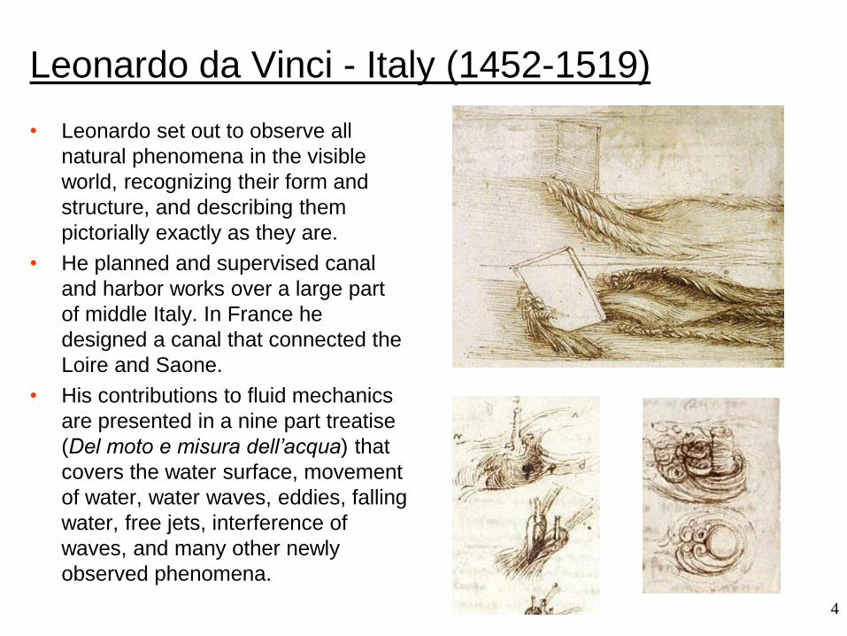
Leonardo da Vinci - Italy (1452-1519)

• Leonardo set out to observe all

natural phenomena in the visible

world, recognizing their form and

structure, and describing them

pictorially exactly as they are.

• He planned and supervised canal

and harbor works over a large part

of middle Italy. In France he

designed a canal that connected the

Loire and Saone.

• His contributions to fluid mechanics

are presented in a nine part treatise

(Del moto e misura dell’acqua) that

covers the water surface, movement

of water, water waves, eddies, falling

water, free jets, interference of

waves, and many other newly

observed phenomena.

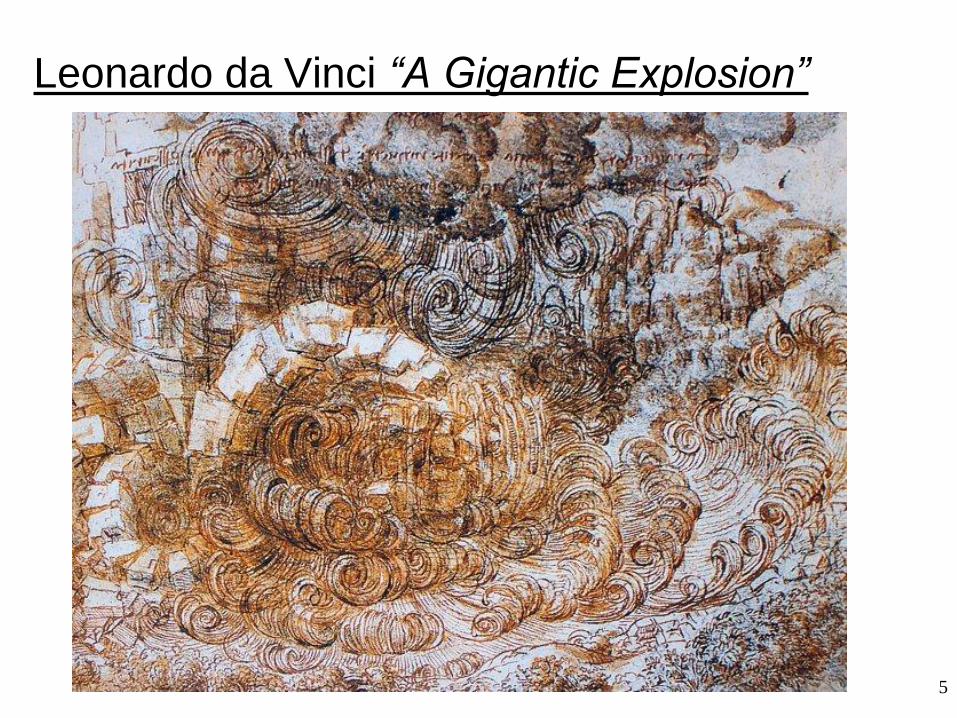
5

Leonardo da Vinci “A Gigantic Explosion”

6

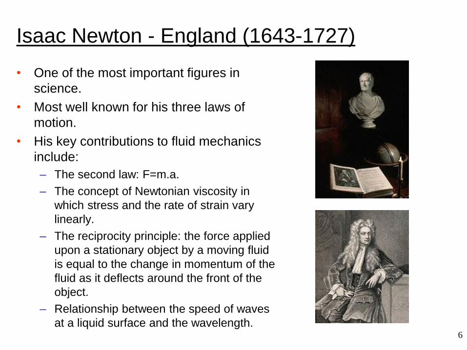
Isaac Newton - England (1643-1727)

• One of the most important figures in

science.

• Most well known for his three laws of

motion.

• His key contributions to fluid mechanics

include:

– The second law: F=m.a.

– The concept of Newtonian viscosity in

which stress and the rate of strain vary

linearly.

– The reciprocity principle: the force applied

upon a stationary object by a moving fluid

is equal to the change in momentum of the

fluid as it deflects around the front of the

object.

– Relationship between the speed of waves

at a liquid surface and the wavelength.

7

• During this period, significant work was done trying to

mathematically describe the motion of fluids.

• Daniel Bernoulli (1700-1782) derived Bernoulli’s equation.

• Leonhard Euler (1707-1783) proposed the Euler equations, which

describe conservation of momentum for an inviscid fluid, and

conservation of mass. He also proposed the velocity potential

theory.

• Claude Louis Marie Henry Navier (1785-1836) and George

Gabriel Stokes (1819-1903) introduced viscous transport into the

Euler equations, which resulted in the Navier-Stokes equation.

This forms the basis of modern day CFD.

• Other key figures were Jean Le Rond d’Alembert, Siméon-Denis

Poisson, Joseph Louis Lagrange, Jean Louis Marie Poiseuille,

John William Rayleigh, M. Maurice Couette, and Pierre Simon de

Laplace.

18th and 19th century

8

Osborne Reynolds - England (1842-1912)

• Reynolds was a prolific writer who

published almost 70 papers during

his lifetime on a wide variety of

science and engineering related

topics.

• He is most well-known for the

Reynolds number, which is the ratio

between inertial and viscous forces

in a fluid. This governs the transition

from laminar to turbulent flow.

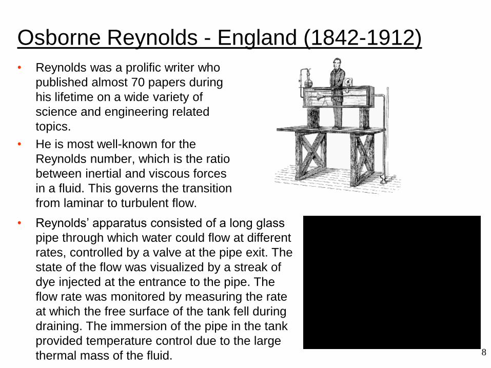
• Reynolds’ apparatus consisted of a long glass

pipe through which water could flow at different

rates, controlled by a valve at the pipe exit. The

state of the flow was visualized by a streak of

dye injected at the entrance to the pipe. The

flow rate was monitored by measuring the rate

at which the free surface of the tank fell during

draining. The immersion of the pipe in the tank

provided temperature control due to the large

thermal mass of the fluid.

9

First part of the 20th century

• Much work was done on refining

theories of boundary layers and

turbulence.

• Ludwig Prandtl (1875-1953):

boundary layer theory, the mixing

length concept, compressible flows,

the Prandtl number, and more.

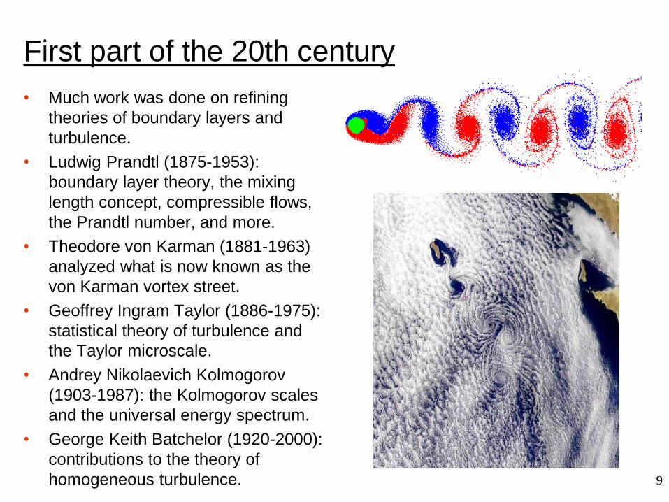
• Theodore von Karman (1881-1963)

analyzed what is now known as the

von Karman vortex street.

• Geoffrey Ingram Taylor (1886-1975):

statistical theory of turbulence and

the Taylor microscale.

• Andrey Nikolaevich Kolmogorov

(1903-1987): the Kolmogorov scales

and the universal energy spectrum.

• George Keith Batchelor (1920-2000):

contributions to the theory of

homogeneous turbulence.

10

Lewis Fry Richardson (1881-1953)

• In 1922, Lewis Fry Richardson developed the first numerical

weather prediction system.

– Division of space into grid cells and the finite difference

approximations of Bjerknes's "primitive differential equations.”

– His own attempt to calculate weather for a single eight-hour period

took six weeks and ended in failure.

• His model's enormous calculation requirements led Richardson to

propose a solution he called the “forecast-factory.”

– The "factory" would have filled a vast stadium with 64,000 people.

– Each one, armed with a mechanical calculator, would perform part of

the calculation.

– A leader in the center, using colored signal lights and telegraph

communication, would coordinate the forecast.

11

1930s to 1950s

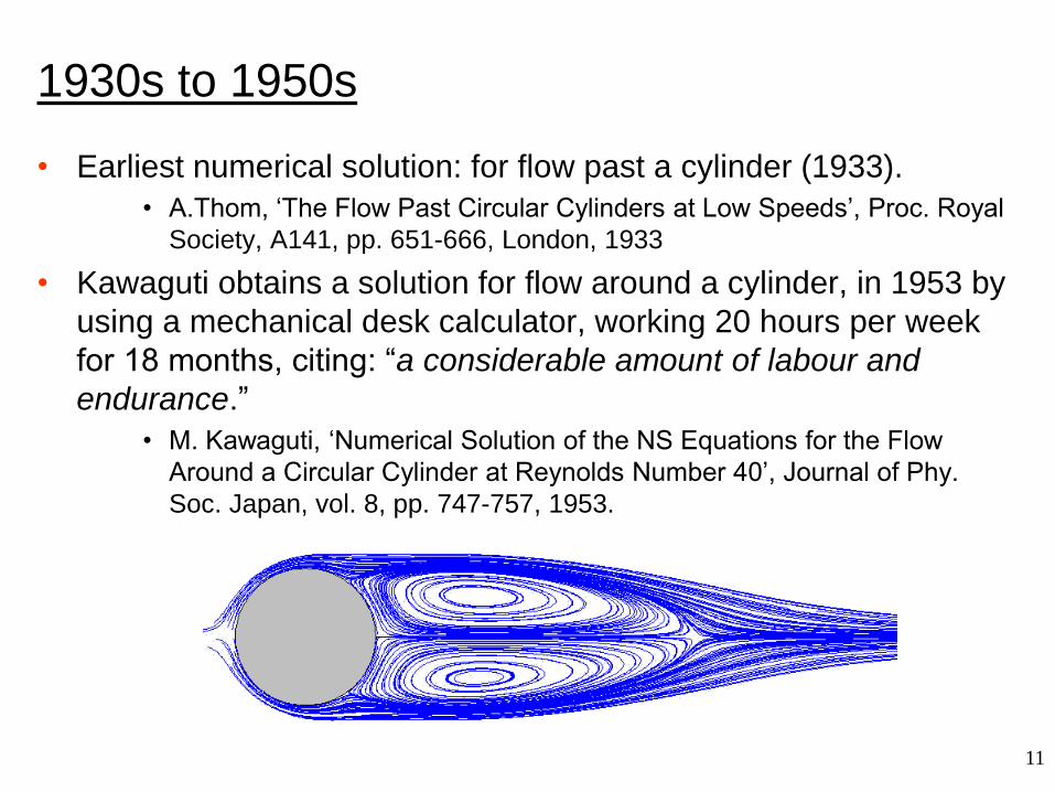
• Earliest numerical solution: for flow past a cylinder (1933).

• A.Thom, ‘The Flow Past Circular Cylinders at Low Speeds’, Proc. Royal

Society, A141, pp. 651-666, London, 1933

• Kawaguti obtains a solution for flow around a cylinder, in 1953 by

using a mechanical desk calculator, working 20 hours per week

for 18 months, citing: “a considerable amount of labour and

endurance.”

• M. Kawaguti, ‘Numerical Solution of the NS Equations for the Flow

Around a Circular Cylinder at Reynolds Number 40’, Journal of Phy.

Soc. Japan, vol. 8, pp. 747-757, 1953.

12

1960s and 1970s

• During the 1960s the theoretical division at Los Alamos contributed many

numerical methods that are still in use today, such as the following methods:

– Particle-In-Cell (PIC).

– Marker-and-Cell (MAC).

– Vorticity-Streamfunction Methods.

– Arbitrary Lagrangian-Eulerian (ALE).

– k- turbulence model.

• During the 1970s a group working under D. Brian Spalding, at Imperial College,

London, develop:

– Parabolic flow codes (GENMIX).

– Vorticity-Streamfunction based codes.

– The SIMPLE algorithm and the TEACH code.

– The form of the k- equations that are used today.

– Upwind differencing.

– ‘Eddy break-up’ and ‘presumed pdf’ combustion models.

• In 1980 Suhas V. Patankar publishes Numerical Heat Transfer and Fluid Flow,

probably the most influential book on CFD to date.

13

1980s and 1990s

• Previously, CFD was performed using academic, research and in-house codes. When one wanted to perform a CFD calculation, one had to write a program.

• This is the period during which most commercial CFD codes originated that are available today: – Fluent (UK and US).

– CFX (UK and Canada).

– Fidap (US).

– Polyflow (Belgium).

– Phoenix (UK).

– Star CD (UK).

– Flow 3d (US).

– ESI/CFDRC (US).

– SCRYU (Japan).

– and more, see www.cfdreview.com.

14

What is computational fluid dynamics?

• Computational fluid dynamics (CFD) is the science of predicting

fluid flow, heat transfer, mass transfer, chemical reactions, and

related phenomena by solving the mathematical equations which

govern these processes using a numerical process.

• The result of CFD analyses is relevant engineering data used in:

– Conceptual studies of new designs.

– Detailed product development.

– Troubleshooting.

– Redesign.

• CFD analysis complements testing and experimentation.

– Reduces the total effort required in the laboratory.

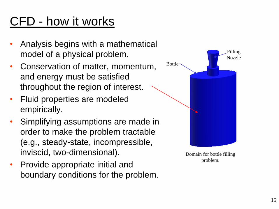
15

Domain for bottle filling

problem.

Filling

Nozzle

Bottle

CFD - how it works

• Analysis begins with a mathematical

model of a physical problem.

• Conservation of matter, momentum,

and energy must be satisfied

throughout the region of interest.

• Fluid properties are modeled

empirically.

• Simplifying assumptions are made in

order to make the problem tractable

(e.g., steady-state, incompressible,

inviscid, two-dimensional).

• Provide appropriate initial and

boundary conditions for the problem.

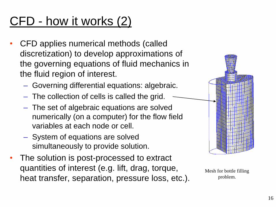
16

Mesh for bottle filling

problem.

CFD - how it works (2)

• CFD applies numerical methods (called

discretization) to develop approximations of

the governing equations of fluid mechanics in

the fluid region of interest.

– Governing differential equations: algebraic.

– The collection of cells is called the grid.

– The set of algebraic equations are solved

numerically (on a computer) for the flow field

variables at each node or cell.

– System of equations are solved

simultaneously to provide solution.

• The solution is post-processed to extract

quantities of interest (e.g. lift, drag, torque,

heat transfer, separation, pressure loss, etc.).

17

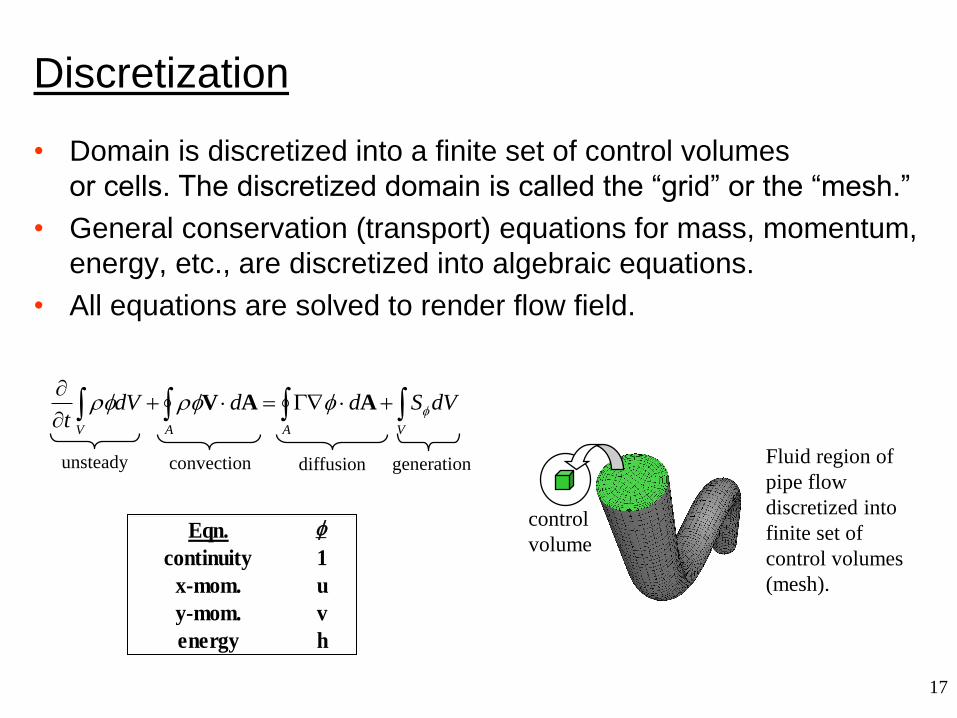
Discretization

• Domain is discretized into a finite set of control volumes

or cells. The discretized domain is called the “grid” or the “mesh.”

• General conservation (transport) equations for mass, momentum,

energy, etc., are discretized into algebraic equations.

• All equations are solved to render flow field.

VAAV

dVSdddVt

AAV

unsteady convection diffusion generation

Eqn.

continuity 1

x-mom. u

y-mom. v

energy h

Fluid region of

pipe flow

discretized into

finite set of

control volumes

(mesh).

control

volume

18

Design and create the grid

• Should you use a quad/hex grid, a tri/tet grid, a hybrid grid, or a

non-conformal grid?

• What degree of grid resolution is required in each region of the

domain?

• How many cells are required for the problem?

• Will you use adaption to add resolution?

• Do you have sufficient computer memory?

triangle

quadrilateral

tetrahedron pyramid

prism or wedge hexahedron arbitrary polyhedron

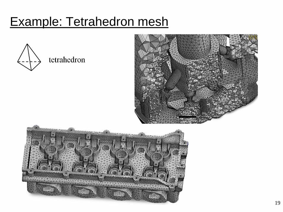
Example: Tetrahedron mesh

19

20

Tri/tet vs. quad/hex meshes

• For simple geometries, quad/hex

meshes can provide high-quality

solutions with fewer cells than a

comparable tri/tet mesh.

• For complex geometries,

quad/hex meshes show no

numerical advantage, and you

can save meshing effort by using

a tri/tet mesh.

21

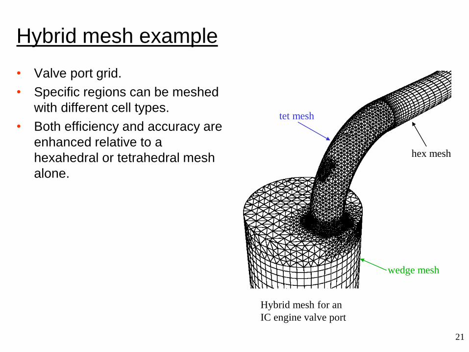
Hybrid mesh example

• Valve port grid.

• Specific regions can be meshed

with different cell types.

• Both efficiency and accuracy are

enhanced relative to a

hexahedral or tetrahedral mesh

alone.

Hybrid mesh for an

IC engine valve port

tet mesh

hex mesh

wedge mesh

22

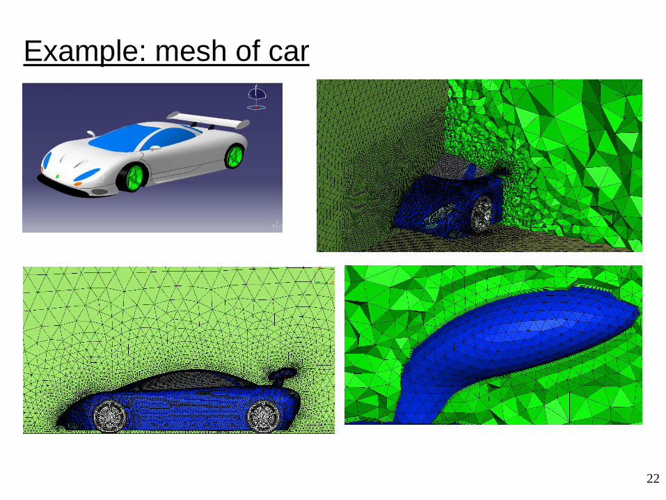
Example: mesh of car

23

Set up the numerical model

• For a given problem, you will need to:

– Select appropriate physical models.

– Turbulence, combustion, multiphase, etc.

– Define material properties.

• Fluid.

• Solid.

• Mixture.

– Prescribe operating conditions.

– Prescribe boundary conditions at all boundary zones.

– Provide an initial solution.

– Set up solver controls.

– Set up convergence monitors.

24

Compute the solution

• The discretized conservation equations are solved iteratively. A

number of iterations are usually required to reach a converged

solution.

• Convergence is reached when:

– Changes in solution variables from one iteration to the next are

negligible.

– Residuals provide a mechanism to help monitor this trend.

– Overall property conservation is achieved.

• The accuracy of a converged solution is dependent upon:

– Appropriateness and accuracy of the physical models.

– Grid resolution and independence.

– Problem setup.

25

Examine the results

• Visualization can be used to answer such questions as:

– What is the overall flow pattern?

– Is there separation?

– Where do shocks, shear layers, etc. form?

– Are key flow features being resolved?

– Are physical models and boundary conditions appropriate?

– Numerical reporting tools can be used to calculate quantitative

results, e.g:

• Lift, drag, and torque.

• Average heat transfer coefficients.

• Surface-averaged quantities.

26

Example: flow over car

CLICK

27

Tools to examine the results

• Graphical tools:

– Grid, contour, and vector plots.

– Pathline and particle trajectory plots.

– XY plots.

– Animations.

• Numerical reporting tools:

– Flux balances.

– Surface and volume integrals and averages.

– Forces and moments.

28

Consider revisions to the model

• Are physical models appropriate?

– Is flow turbulent?

– Is flow unsteady?

– Are there compressibility effects?

– Are there 3D effects?

– Are boundary conditions correct?

• Is the computational domain large enough?

– Are boundary conditions appropriate?

– Are boundary values reasonable?

• Is grid adequate?

– Can grid be adapted to improve results?

– Does solution change significantly with adaption, or is the solution

grid independent?

– Does boundary resolution need to be improved?

29

Applications of CFD

• Applications of CFD are numerous!

– Flow and heat transfer in industrial processes (boilers, heat

exchangers, combustion equipment, pumps, blowers, piping, etc.).

– Aerodynamics of ground vehicles, aircraft, missiles.

– Film coating, thermoforming in material processing applications.

– Flow and heat transfer in propulsion and power generation systems.

– Ventilation, heating, and cooling flows in buildings.

– Chemical vapor deposition (CVD) for integrated circuit

manufacturing.

– Heat transfer for electronics packaging applications.

– And many, many more!

Applications of CFD

30

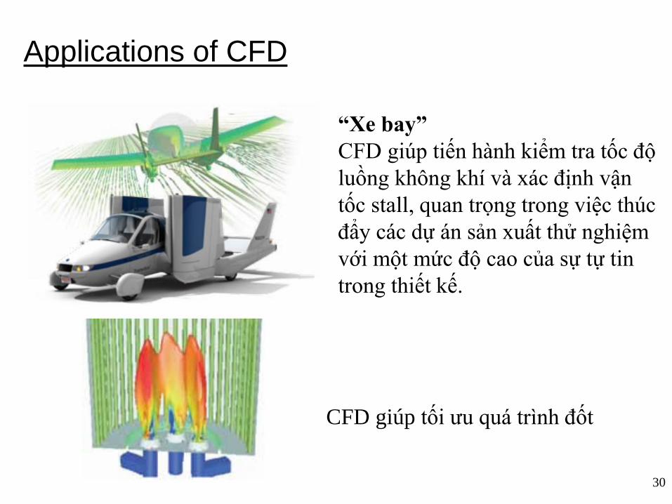
“Xe bay”

CFD giúp tiến hành kiểm tra tốc độ

luồng không khí và xác định vận

tốc stall, quan trọng trong việc thúc

đẩy các dự án sản xuất thử nghiệm

với một mức độ cao của sự tự tin

trong thiết kế.

CFD giúp tối ưu quá trình đốt

Applications of CFD

31

Ứng dụng trong

thiết kế xe

Năng lượng

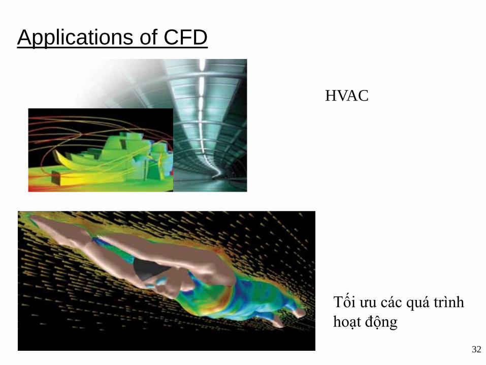
Applications of CFD

32

HVAC

Tối ưu các quá trình

hoạt động

33

Advantages of CFD

• Relatively low cost.

– Using physical experiments and tests to get essential engineering

data for design can be expensive.

– CFD simulations are relatively inexpensive, and costs are likely to

decrease as computers become more powerful.

• Speed.

– CFD simulations can be executed in a short period of time.

– Quick turnaround means engineering data can be introduced early in

the design process.

• Ability to simulate real conditions.

– Many flow and heat transfer processes can not be (easily) tested,

e.g. hypersonic flow.

– CFD provides the ability to theoretically simulate any physical

condition.

34

Advantages of CFD (2)

• Ability to simulate ideal conditions.

– CFD allows great control over the physical process, and provides the

ability to isolate specific phenomena for study.

– Example: a heat transfer process can be idealized with adiabatic,

constant heat flux, or constant temperature boundaries.

• Comprehensive information.

– Experiments only permit data to be extracted at a limited number of

locations in the system (e.g. pressure and temperature probes, heat

flux gauges, LDV, etc.).

– CFD allows the analyst to examine a large number of locations in the

region of interest, and yields a comprehensive set of flow parameters

for examination.

35

Limitations of CFD

• Physical models.

– CFD solutions rely upon physical models of real world processes

(e.g. turbulence, compressibility, chemistry, multiphase flow, etc.).

– The CFD solutions can only be as accurate as the physical models

on which they are based.

• Numerical errors.

– Solving equations on a computer invariably introduces numerical

errors.

– Round-off error: due to finite word size available on the computer.

Round-off errors will always exist (though they can be small in most

cases).

– Truncation error: due to approximations in the numerical models.

Truncation errors will go to zero as the grid is refined. Mesh

refinement is one way to deal with truncation error.

36

poor better

Fully Developed Inlet

Profile

Computational

Domain

Computational

Domain

Uniform Inlet

Profile

Limitations of CFD (2)

• Boundary conditions.

– As with physical models, the accuracy of the CFD solution is only as

good as the initial/boundary conditions provided to the numerical

model.

– Example: flow in a duct with sudden expansion. If flow is supplied to

domain by a pipe, you should use a fully-developed profile for

velocity rather than assume uniform conditions.

37

Summary

• CFD is a method to numerically calculate heat transfer and fluid

flow.

• Currently, its main application is as an engineering method, to

provide data that is complementary to theoretical and

experimental data. This is mainly the domain of commercially

available codes and in-house codes at large companies.

• CFD can also be used for purely scientific studies, e.g. into the

fundamentals of turbulence. This is more common in academic

institutions and government research laboratories. Codes are

usually developed to specifically study a certain problem.