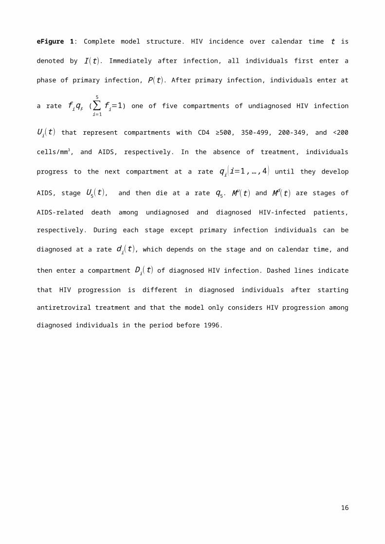
Estimating HIV incidence, time to diagnosis, and the undiagnosed HIV epidemic using routine

surveillance data

eAppendix

Model structure

The full structure of our model is shown in eFigure 1. The model is a deterministic

compartmental model that describes HIV progression in the absence of antiretroviral treatment

as a unidirectional flow through different stages of the infection. The HIV incidence over

calendar time t is given by I (t), which is unknown and needs to be estimated by fitting the

model to observed data. Immediately after infection, all individuals first enter a phase of

primary infection, P(t). After primary infection, individuals enter at a rate f iqP one of five

compartments U i(t )( i=1 ,…,5 ) of undiagnosed HIV infection with ∑i=1

5

f i=1. The first four stages

U1 ( t ) to U4 (t ) correspond to CD4 strata ≥500, 350-499, 200-349, and <200 cells/mm3,

respectively, in the absence of an AIDS-defining illness, whilst U 5(t ) corresponds to AIDS

irrespective of CD4 count.

During each stage U i(t ) of undiagnosed HIV infection, patients can be diagnosed at a rate d i(t)

, which depends on the stage of infection and on calendar time. Upon diagnosis, patients enter

a stage Di(t) of diagnosed HIV infection. In the absence of antiretroviral treatment, both

undiagnosed and diagnosed patients experience the same rate of progression to the next CD4

stratum. Progression in diagnosed patients will be different after they start treatment.

Therefore, the model only describes HIV progression in undiagnosed patients or in diagnosed

patients before the introduction of combination antiretroviral treatment in 1996.

Model equations

The model is formulated as a set of ordinary differential equations that describe the changes

over time t in the number of individuals in each compartment in eFigure 1. The equations are

1

solved numerically using a fourth order Runge-Kutta algorithm. Parameter values are given in

eTable 1.

dP ( t )dt

=I ( t )−qPP ( t )−μP(t )dU 1 (t )dt

=f 1qPP ( t )−q1U 1 ( t )−d1 (t )U1 (t )−μU1(t )

dU i (t )dt

=f i qP P (t )−qiU i (t )+q i−1U i−1 (t )−d i ( t )U i (t )−μU i(t) (i=2 ,…,5 )

d D1 (t )dt

=d1 (t )U1 (t )−q1D1 (t )d Di (t )dt

=d i ( t )U i (t )−q iDi (t )+qi−1D i−1 (t )(i=2 ,…,5)

The change in the total number of individuals diagnosed in each stage, Didiag (t )(i=1 ,…5), is

given by

d Didiag (t )dt

=d i (t )U i(t)

Before 1996 when combination antiretroviral treatment became available, the cumulative

number of individuals diagnosed with AIDS, Ad (t), consists of those with a concurrent HIV and

AIDS diagnosis (stage U5(t ) to D5(t)) and diagnosed individuals who progress to AIDS (stage

D4 (t) to D5(t)). Therefore,

d Ad ( t )dt

=d5 ( t )U5 (t )+q4D 4(t )

The number of infected men who die without being diagnosed, M u(t), is given by

dM u(t )dt

=μP (t )+∑i=1

5

μU i ( t )+¿q5U 5(t )¿

2

Taking into account missing CD4 measurements and the probability that diagnosed individuals

survive up to 1996, the observed number Diobs(t) of HIV diagnoses in each CD4 stratum i is

written as

Diobs ( t )=Di ( t ) pi

CD 4 (t ) si(t )

where piCD 4(t ) is the probability of having a CD4 count measurement available when diagnosed

in CD4 stratum i in calendar year t and si(t) is the probability that an untreated individual

diagnosed in CD4 stratum i in calendar year t will survive up to 1996.

Equation for time from infection to diagnosis

The average time from infection to diagnosis, t diag, if diagnosis rates remain the same as at the

time of infection t , can be calculated as

t diag=1qP

+∑k=1

5

f k∑j=k

5 d j(t )q j+d j(t) (∏s=k

j−1 qsqs+ds( t) )∑i=k

j 1q i+d i(t)

This equation is the sum of the average duration of all possible pathways in eFigure 1 from

infection to each of the five stages of diagnosed HIV infection Di(t) weighted by the probability

of taking each pathway. The first term 1/qP at the right hand side of the equation is the

average duration of primary infection. In the second term, d j(t)/ (q j+d j(t)) is the probability of

being diagnosed whilst in stage U j(t) and thus going to D j(t), qs / (qs+ds( t)) is the probability of

remaining undiagnosed and progressing from U s(t) to U s+1(t), and 1/ (q i+d i(t)) is the average

duration patients stay in stage U i(t ).

The actual time from infection to diagnosis, t diagactual, i.e., the duration patients have been infected

by the time they are diagnosed in year t d, is approximated by

3

t diagactual (t d )= 1

D(t d)∑k=1

5

∑s=1

d

D ks (t d ) (d−s−0.5)

where D(t d) is the total number of HIV diagnoses in year t d, and Dks (t d) is the number of HIV

diagnoses in stage k and year t d among individuals infected in year t s.

HIV incidence curve

The HIV incidence curve is approximated using cubic M-splines, which are piecewise

polynomials of degree 4 defined by a knot sequence (t 1 ,…, tK ) ,K=k+8, where k is the number

of internal knots. The knot sequence is defined such that t 1≤…≤t k +8, t 1=…=t 4=L, and

t k+5=…=t k+8=U where L is 1 January 1980 and U is 31 December 2012. M-splines are defined

such that spline M i(i=1 ,…,k+4) is positive in the interval (t i , t i+4) and zero elsewhere and has

the normalisation ∫M i (t )dt=1. Adjacent splines are required to join at the boundaries of the

intervals with equal first-order derivatives and continuous second-order derivatives. Formulae

for M-spline M i(t) are taken from Ramsay [1]. The incidence curve I (t) is approximated by a

linear combination of the k+4 M-splines: I (t )=∑i=1

k+4

ϑ iM i(t) with parameters ϑ i that need to be

estimated by fitting to data [2]. We take the k internal knots to be equidistant between L and

U , whilst k is chosen such that fewer knots would give a model with a worse fit to the data.

Diagnosis because of HIV-related symptoms

In a secondary analysis, we assume that diagnosis rates are the same for the first three CD4

strata (d1 ( t )=d2 (t )=d3( t)) and that d4 (t )=d3 ( t )+dsymp(t) with dsymp( t) the rate of being

diagnosed because of HIV-related symptoms. The rate of developing HIV-related symptoms is

approximately double the rate of AIDS, i.e. 2×q4 [3-5]. However, not all HIV-related symptoms

are severe enough to lead to testing for HIV [6,7]. We therefore assume that 50% of HIV

4

infections with symptoms are missed, such that d symp( t)=50%×2×q4≈ 0.4 per year, which is

approximately 50% of the rate of HIV-related symptoms (eTable 1).

Fitting procedure

As described in the main text, the model needs to estimate 16 parameters relating to the

probability of HIV diagnosis and k+4 parameters ϑ i(i=1,…,k+4) associated with the

incidence curve, which is modelled as a superposition of k+4 cubic M-splines, where k is the

number of internal knots. Maximum likelihood methods are used to find the set of parameters

that best fit the observed data. To define the likelihood, we assume that all data items are

distributed according to a negative binomial distribution around a mean defined by the model

and a dispersion parameter r which is initially set at a value of 1000. For convenience, instead

of maximising the likelihood, we minimise the equivalent deviance measure. A downhill simplex

optimisation algorithm is used to find the minimum value. The algorithm is started from various

starting values to ensure that the optimisation is robust and that local optima are avoided.

In the first step of the fitting procedure, all parameters are estimated except for ϑ1 which is

fixed to 0 in order to ensure that the incidence curve starts at zero. To improve the robustness

and convergence of the fitting procedure, any ϑ i(i=2 ,… ,k+3) whose estimated value is either

less than 1 or less than a fraction f (chosen to be 5%) of the estimated value for ϑ i+1 is fixed at

zero. All parameters are then re-estimated and this procedure is repeated until no more ϑ i fulfil

these criteria. Note that the coefficient associated with the k+4-th spline is allowed to be

smaller than 1, because fixing it at zero would force the incidence to be zero.

In the second step, a new approximate value for the dispersion parameter is obtained by

requiring that Pearson’s χ2 statistic equals n−p with n the number of data points used in the fit

and p the number of estimated parameters [8]. Using this updated dispersion parameter r the

set of parameters is re-estimated. This procedure is repeated until the dispersion parameter

does not notably change anymore, which is the case after four times.

5

Confidence intervals

We estimated pointwise 95% confidence intervals for parameters and other derived quantities

via a bootstrap procedure [9]. In brief, assuming that the data are distributed according to a

negative binomial with a mean defined by the model, we generated a new dataset by sampling

from this distribution for every year for each of the relevant data items. The model was then

refitted to this new dataset starting from the parameter values found in the main fit. This

sampling and refitting procedure was repeated 200 times. From these 200 fits, 95% confidence

intervals around the main model fit were then determined as the 2.5th and 97.5th percentile.

Simulated data

Our approach was tested on three data sets of hypothetical patients generated by the HIV

Synthesis progression model [10,11]. These hypothetical patients represented HIV epidemics

for different risk groups in a typical European country generated with different pairs of

incidence and diagnosis rate curves. For each diagnosed patient, the CD4 count at diagnosis

was known, as well as the date of AIDS diagnosis, death, and date of emigration or loss to

follow-up. Our model was tested by comparing the reconstructed HIV incidence curve with the

true annual number of HIV infections that was used as an input in the simulation. Hypothetical

patients who migrated before being diagnosed were not included in the true number of

infections. When information on CD4 counts at the time of diagnosis was not included in the

model, the estimated HIV infection curve looked very similar (eFigure 2 and 3).

Model fits

eFigures 4A and 4B show the curves that best fitted to the observed data on AIDS cases and

HIV/AIDS diagnoses, as well as on annual total number of HIV diagnoses, reflecting the steep

increase in annual HIV infections and shorter time to diagnosis. eFigure 5 shows the best-fitting

curves to the number of new HIV diagnoses by CD4 stratum. Before 1996, the proportion of

patients with a CD4 count was 34%; this increased to over 85% in recent years. The proportion

6

of MSM with a measured CD4 count ≥500 cells/mm3 at the time of HIV diagnosis increased

from 17% in 1996 to 38% in 2012.

eFigure 6 shows the estimated model outcomes when diagnosis rates in the period 1984-1995

were assumed to be a linear function of calendar time instead of being constant. The estimated

annual number of HIV infections (eFigure 6A) was comparable to the main analysis, as was the

cumulative number of 15,300 (95% CI, 14,800-16,000) infections by the end of 2011. As

expected, the estimated average time from infection to diagnosis by year of infection was

different for the period 1984-1995. eFigure 7 shows the estimated diagnosis rates by CD4

count interval. From 1996 onwards, diagnosis rates were very similar between the two models,

with the steep increase reflecting adoption of a more active HIV testing strategy after the

availability of combination antiretroviral therapy [12].

The HIV infection curve looked very similar although with wider confidence intervals in more

recent calendar years when no information on CD4 counts at the time of diagnosis was used

(eFigure 8A). The cumulative number of infections by the end of 2011 was 15,500 (95% CI,

14,700-16,200), which was comparable to the model with information on CD4 counts. The

estimated time to diagnosis was also similar, 2.8 (2.4-3.4) years in 2011 (eFigure 8B).

Multivariable sensitivity analysis

We did a multivariable sensitivity analysis to investigate the impact of assumptions on input

parameters on the model outcomes. For each of the input parameters, a range of plausible

values was identified (eTable 1). Each parameter was partitioned into 250 equidistant possible

values spanning its whole plausible range. The sensitivity of the model to the fixed input

parameters was then evaluated by sampling from all possible parameter values. Parameter

values were sampled using Latin hypercube sampling such that each possible value was

sampled exactly once [13,14]. For each parameter set, we refitted the model to the data and

re-estimated the unknown parameters. In this way we explored a wide range of input

parameters, but only with the restricted set of scenarios that best fit the observed data [14].

7

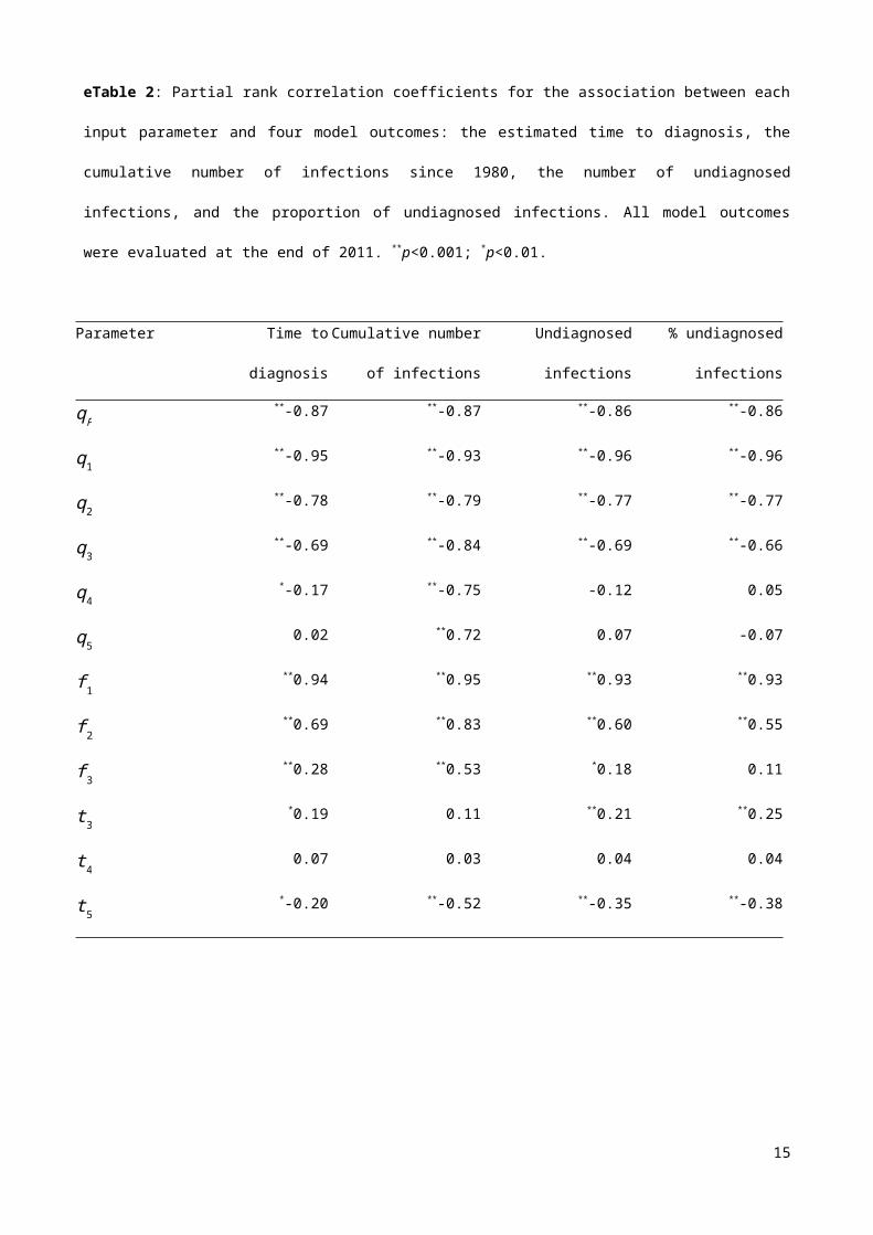
Partial rank correlation coefficients (PRCCs) were calculated for the correlation between each

input parameter and four model outputs: the estimated time to diagnosis, the cumulative

number of HIV infections, and the number and proportion of undiagnosed infections. In general,

PRCC values near 1 (or -1) indicate a strong positive (or negative) influence of the input

parameter on the estimated model output, whilst values near 0 indicate little influence.

Higher disease progression rates were generally associated with a shorter estimated time to

diagnosis as indicated by negative PRCCs (eTable 2). To understand these associations it

should be noted that a higher value of qP means a shorter duration of primary infection and

hence a shorter time to diagnosis. A higher rate of progressing to the next CD4 stratum is

compensated for by a higher diagnosis rate, and thus a shorter time to diagnosis, for the

current CD4 stratum in order for the model to generate a certain number of HIV diagnoses that

can be compared with observed data. An analogous argument explains the positive correlation

between the proportion in each disease stage immediately after primary infection and the time

to diagnosis. A higher proportion of patients entering a disease stage needs to be compensated

by a lower diagnosis rate and hence a longer time between infection and diagnosis. Parameters

related to the early stages of HIV infection had the largest influence on estimated time to

diagnosis.

Similar associations were observed between input parameters and the number of infections.

Since faster disease progression is compensated for by a shorter time to diagnosis, new HIV

infections will be diagnosed more rapidly. Hence, the estimated number of infections is smaller

in order to generate the same number of HIV diagnoses. As a consequence, the proportion of

undiagnosed infections will also be smaller.

Missing CD4 counts

In the main model we implicitly assumed that CD4 counts were missing at random such that

patients without CD4 count measurement had the same CD4 distribution as those with a CD4

measurement. Simulated data were used to assess the effect of missing CD4 data by randomly

or non-randomly deleting certain proportions of the observed number of HIV diagnoses per CD4

8

count stratum and then repeating the model fits assuming that CD4 counts were missing at

random. We considered various scenarios: (i) CD4 counts missing at random for 10% to 90% of

all HIV diagnoses in steps of 10%, (ii) CD4 counts missing for 10% to 90% of HIV diagnoses with

CD4 count <200 cells/mm3 (stage 4 in eFigure 1) and for smaller but equal proportions for the

other three CD4 stages. For both types of scenarios, estimates of the annual number of HIV

infections for all three simulated HIV epidemics were within the confidence intervals estimated

in the main mode. The estimated time between infection to diagnosis by year of infection or by

year of diagnosis was almost identical and well with the confidence intervals for scenario (i).

However, for scenario (ii) estimates of time to diagnosis were consistently lower, up to 50% or

2 years, the higher the proportion of missing CD4 counts in stage 4 and the larger the

difference between the proportions missing in stage 4 and the other three stages. This is

because by (wrongly) assuming that CD4 counts were missing at random, the annual number

of diagnoses with CD4 count <200 cells/mm3 is underestimated while the number of diagnoses

in the other three CD4 strata is overestimated. Thus, the time between infection and diagnosis

appears to be shorter.

9

eTable 1: Parameters used in the mathematical model for estimating HIV incidence and

diagnosis rates. The range of qP was the reported 95% confidence interval. For the other rates

q i(i=1 ,…,5) the range was chosen to be 0.8 to 1.2 times the main value. Years are continuous

variables with whole years representing 1 January-31 December. In the sensitivity analyses,

new values were sampled within the given ranges using Latin hypercube sampling. Rates are

per year.

Description Symbol Value Range Source

Rate of progression from

acute to chronic infection

(per year)

qP 4.14 2.00 – 9.76 [15]

Proportion in each disease

stage directly after primary

infection

f 1 0.58 ¿1−f 2−f 3−f 4−f 5 [16,17]

f 2 0.23 0.19 – 0.27 [16,17]

f 3 0.16 0.14 – 0.18 [16,17]

f 4 0.03 0.00 – 0.05 [16,17]

f 5 0 –

Rate of progression to the

next disease stage (per

year)

q1 1/6.37 0.13 – 0.19 [16,17]

q2 1/2.86 0.28 – 0.42 [16,17]

q3 1/3.54 0.23 – 0.34 [16,17]

q4 1/2.30 0.35 – 0.52 [16,17]

Rate of progression from

AIDS to death (per year)

q5 1/1.89 0.42 – 0.63 [18,19]

Diagnosis rate by disease

stage (per year)

d1(t) estimated – –

d2(t) estimated – –

10

d3(t ) estimated – –

d4 (t) estimated – –

d5(t ) 12 – [18,19]

dsymp( t) 0 (t<1984), – assumption

0.4 (t≥1984) 0.2 – 0.6 assumption

Mortality rate due to causes

other than HIV (per year)

μ 0 – assumption

Start year of historical

intervals for diagnosis rates

t 1 1980 –

t 2 1984 –

t 3 1996 1995 – 1997

t 4 2000 1999 – 2001

t 5 2005 2004 – 2006

Number of internal knots k 2 to 6 –

11

eTable 2: Partial rank correlation coefficients for the association between each input

parameter and four model outcomes: the estimated time to diagnosis, the cumulative number

of infections since 1980, the number of undiagnosed infections, and the proportion of

undiagnosed infections. All model outcomes were evaluated at the end of 2011. **p<0.001; *p<0.01.

Parameter Time to diagnosis Cumulative number

of infections

Undiagnosed

infections

% undiagnosed

infections

qP**-0.87 **-0.87 **-0.86 **-0.86

q1**-0.95 **-0.93 **-0.96 **-0.96

q2**-0.78 **-0.79 **-0.77 **-0.77

q3**-0.69 **-0.84 **-0.69 **-0.66

q4*-0.17 **-0.75 -0.12 0.05

q5 0.02 **0.72 0.07 -0.07

f 1**0.94 **0.95 **0.93 **0.93

f 2**0.69 **0.83 **0.60 **0.55

f 3**0.28 **0.53 *0.18 0.11

t 3*0.19 0.11 **0.21 **0.25

t 4 0.07 0.03 0.04 0.04

t 5*-0.20 **-0.52 **-0.35 **-0.38

12

eFigure 1: Complete model structure. HIV incidence over calendar time t is denoted by I (t).

Immediately after infection, all individuals first enter a phase of primary infection, P(t). After

primary infection, individuals enter at a rate f iqP (∑i=1

5

f i=1) one of five compartments of

undiagnosed HIV infection U i(t ) that represent compartments with CD4 ≥500, 350-499, 200-

349, and <200 cells/mm3, and AIDS, respectively. In the absence of treatment, individuals

progress to the next compartment at a rate q i ( i=1 ,…,4 ) until they develop AIDS, stage U 5(t ),

and then die at a rate q5. M u(t) and M d(t ) are stages of AIDS-related death among

undiagnosed and diagnosed HIV-infected patients, respectively. During each stage except

primary infection individuals can be diagnosed at a rate d i(t), which depends on the stage and

on calendar time, and then enter a compartment Di(t) of diagnosed HIV infection. Dashed lines

indicate that HIV progression is different in diagnosed individuals after starting antiretroviral

treatment and that the model only considers HIV progression among diagnosed individuals in

the period before 1996.

13

eFigure 2: Estimated and true number of infections for three different simulated HIV

epidemics when fitting to the total annual number of HIV diagnoses instead of diagnoses by

CD4 count stratum. Black solid lines show the model estimates, and dashed lines are 95%

confidence intervals. Thin grey lines show results of multivariable sensitivity analyses. Grey

dots are the true annual number of infections that were used as input in the simulations.

14

eFigure 3: Estimated and true number of undiagnosed infections for three different simulated

HIV epidemics when fitting to the total annual number of HIV diagnoses instead of diagnoses

by CD4 count stratum. Black solid lines show the model estimates, and dashed lines are 95%

confidence intervals. Thin grey lines show results of multivariable sensitivity analyses. Grey

dots are the true annual proportions undiagnosed infections.

15

eFigure 4: Model fits to reported HIV and AIDS cases in MSM in the Netherlands. (A) Annual

number of new AIDS cases (+ signs) and concurrent HIV and AIDS diagnoses (dots); (B) annual

number of HIV diagnoses. Black solid lines show the best model fit to the data, whilst black

dashed lines are 95% confidence intervals. Black shapes are data points used for fitting, grey

shapes are not used for fitting. Thin grey lines show results of multivariable sensitivity

analyses. In panel B, the thick dashed grey line is the model estimate for the actual number of

HIV diagnoses taking into account patients who did not survive up to 1996.

16

eFigure 5: Model fits to reported HIV diagnoses by CD4 count. The panels show the annual

number of observed HIV diagnoses (black dots) with CD4 counts (A) ≥500 cells/mm3, (B) 350-

499 cells/mm3, (C) 200-349 cells/mm3, and (D) <200 cells/mm3. Black solid lines show the

model fit, and dashed lines are 95% confidence intervals. Thick grey lines are the actual

number of HIV diagnoses taking into account patients who did not survive up to 1996 and

patients for whom no CD4 was available. Thin grey lines show results of multivariable

sensitivity analyses.

17

eFigure 6: Model outcomes for men who have sex with men (MSM) in the Netherlands when

diagnosis rates in the period 1984-1995 were assumed to be a linear function of calendar time.

(A) Annual number of new HIV infections; (B) average time from HIV infection to diagnosis by

year of infection if diagnosis rates would remain the same as in the year of infection; (C)

average time from HIV infection to diagnosis by year of diagnosis; (D) total number of

individuals living with HIV and number of diagnosed and undiagnosed HIV infections, with dots

representing the number of diagnosed MSM living with HIV according to the AIDS Therapy

Evaluation in the Netherlands (ATHENA) database. Dashed grey lines in (A), (B), and (C) are

results for the main model with constant diagnosis rate in 1984-1995, while thin grey lines

show results of multivariable sensitivity analyses.

18

eFigure 7: Estimated diagnosis rates for the four CD4 count intervals (A) ≥500 cells/mm3, (B)

350-499 cells/mm3, (C) 200-349 cells/mm3, and (D) <200 cells/mm3. Solid lines show the

estimated diagnosis rate, and dashed lines are 95% confidence intervals. Black lines are results

when assuming a constant diagnosis rate in the period 1984-1995, while grey lines represent

results when assuming a linear function of calendar time.

19

eFigure 8: Model outcomes for men who have sex with men in the Netherlands when no

information on CD4 counts was used. (A) Annual number of new HIV infections; (B) average

time from HIV infection to diagnosis by year of infection if parameters would not change. Black

solid lines show the best model fit to the data, whilst black dashed lines are 95% confidence

intervals. Thin grey lines show results of multivariable sensitivity analyses.

20

References

1. Ramsay JO. Monotone Regression Splines in Action. Statistical Science 1988; 3:425-441.

2. Alioum A, Commenges D, Thiebaut R, Dabis F. A multistate approach for estimating the

incidence of human immunodeficiency virus by using data from a prevalent cohort study.

Appl Statist 2005; 54:739-752.

3. Lee CA, Phillips AN, Elford J, Janossy G, Griffiths P, Kernoff P. Progression of HIV disease in

a haemophilic cohort followed for 11 years and the effect of treatment. BMJ 1991;

303:1093-1096.

4. Morgan D, Mahe C, Mayanja B, Whitworth JA. Progression to symptomatic disease in

people infected with HIV-1 in rural Uganda: prospective cohort study. BMJ 2002; 324:193-

196.

5. Flegg PJ. Barnett Christie Lecture (1993). The natural history of HIV infection: a study in

Edinburgh drug users. J Infect 1994; 29:311-321.

6. Schouten M, van Velde AJ, Snijdewind IJ, Verbon A, Rijnders BJ, van der Ende ME. [Late

diagnosis of HIV positive patients in Rotterdam, the Netherlands: risk factors and missed

opportunities]. Ned Tijdschr Geneeskd 2013; 157:A5731.

7. British HIV Association Audit & Standards Sub-Committee. 2010-11 survey of HIV testing

policy and practice and audit of new patients when first seen post-diagnosis. 2011

Available at:

www.bhiva.org/documents/ClinicalAudit/FindingsandReports/HIVdiagnosisWebVersion.ppt.

8. Mccullagh P. Quasi-Likelihood Functions. Annals of Statistics 1983; 11:59-67.

9. Efron B, Tibshirani RJ. An Introduction to the Bootstrap. New York: Chapman & Hall/CRC,

1993.

10. Phillips AN, Sabin C, Pillay D, Lundgren JD. HIV in the UK 1980-2006: reconstruction using

a model of HIV infection and the effect of antiretroviral therapy. HIV Med 2007; 8:536-

546.

21

11. Phillips AN, Cambiano V, Nakagawa F et al. Increased HIV incidence in men who have sex

with men despite high levels of ART-induced viral suppression: analysis of an extensively

documented epidemic. PLoS ONE 2013; 8:e55312.

12. Health Council of the Netherlands: Standing Committee on Infectious Diseases and

Immunology. Reconsidering the policy on HIV testing. Publication no. 1999/02. The Hague,

Health Council of the Netherlands, 1999.

13. Sanchez MA, Blower SM. Uncertainty and sensitivity analysis of the basic reproductive

rate. Tuberculosis as an example. Am J Epidemiol 1997; 145:1127-1137.

14. van Sighem A, Vidondo B, Glass TR et al. Resurgence of HIV infection among men who

have sex with men in Switzerland: mathematical modelling study. PLoS ONE 2012;

7:e44819.

15. Hollingsworth TD, Anderson RM, Fraser C. HIV-1 transmission, by stage of infection. J

Infect Dis 2008; 198:687-693.

16. Lodi S, Phillips A, Touloumi G et al. Time from human immunodeficiency virus

seroconversion to reaching CD4+ cell count thresholds <200, <350, and <500

Cells/mm(3): assessment of need following changes in treatment guidelines. Clin Infect

Dis 2011; 53:817-825.

17. Cori A, Ayles H, Beyers N et al. HPTN 071 (PopART): A Cluster-Randomized Trial of the

Population Impact of an HIV Combination Prevention Intervention Including Universal

Testing and Treatment: Mathematical Model. PLoS ONE 2014; 9:e84511.

18. Bezemer D, de Wolf F, Boerlijst MC et al. A resurgent HIV-1 epidemic among men who

have sex with men in the era of potent antiretroviral therapy. AIDS 2008; 22:1071-1077.

19. Bezemer D, de Wolf F, Boerlijst MC, van Sighem A, Hollingsworth TD, Fraser C. 27 years of

the HIV epidemic amongst men having sex with men in the Netherlands: an in depth

mathematical model-based analysis. Epidemics 2010; 2:66-79.

22

23