ˇ ˙ ˘˛ˇ ˇ ˚ ˆ˙ ˘ ˛ˇ - nber.org · 1 Introduction The “geography hypothesis”...
83
1%(5:25.,1*3$3(56(5,(6 5(9(56$/2))25781( *(2*5$3+<$1',167,787,216,17+(0$.,1*2)7+( 02'(51:25/',1&20(',675,%87,21 'DURQ$HPRJOX 6LPRQ-RKQVRQ -DPHV$5RELQVRQ :RUNLQJ3DSHU KWWSZZZQEHURUJSDSHUVZ 1$7,21$/%85($82)(&2120,&5(6($5&+ 0DVVDKXVHWWV$YHQXH &DPEULGJH0$ 6HSWHPEHU :HWKDQN-RVKXD$QJULVW$EKLMLW%DQHUMHH2OLYLHU%ODQKDUG$OHVVDQGUD&DVVHOOD-DQGH9ULHV5RQ )LQGOD\+HUVKHO*URVVPDQ/DZUHQH.DW]3HWHU/DQJH)DEUL]LR=LOLERWWLDQGVHPLQDUSDUWLLSDQWVDW WKH$OO8&+LVWRU\&RQIHUHQHDW%HUNHOH\WKHRQIHUHQHRQ³*OREDOL]DWLRQDQG0DUJLQDOL]DWLRQ´LQ %HUJHQ 7KH &DQDGLDQ ,QVWLWXWH RI $GYDQHG 5HVHDUK &KLDJR &ROXPELD '(/7$ 0,7 1%(5 VXPPHULQVWLWXWH6WDQIRUGDQG<DOHIRUXVHIXORPPHQWV$HPRJOXJUDWHIXOO\DNQRZOHGJHVILQDQLDO KHOSIURP7KH&DQDGLDQ,QVWLWXWHIRU$GYDQHG5HVHDUKDQGWKH1DWLRQDO6LHQH)RXQGDWLRQ*UDQW 6(6-RKQVRQWKDQNVWKH0,7(QWUHSUHQHXUVKLS&HQWHUIRUVXSSRUW7KHYLHZVH[SUHVVHGKHUHLQ DUHWKRVHRIWKHDXWKRUVDQGQRWQHHVVDULO\WKRVHRIWKH1DWLRQDO%XUHDXRI(RQRPL5HVHDUK E\'DURQ$HPRJOX6LPRQ-RKQVRQDQG-DPHV$5RELQVRQ$OOULJKWVUHVHUYHG6KRUWVHWLRQVRIWH[W QRWWRH[HHGWZRSDUDJUDSKVPD\EHTXRWHGZLWKRXWH[SOLLWSHUPLVVLRQSURYLGHGWKDWIXOOUHGLWLQOXGLQJ QRWLHLVJLYHQWRWKHVRXUH
Transcript of ˇ ˙ ˘˛ˇ ˇ ˚ ˆ˙ ˘ ˛ˇ - nber.org · 1 Introduction The “geography hypothesis”...

�������������������������
����������������
������������������������������������������
������������������������������
����������� !"
�#����$�%�&��
$���&��'���(#�&��
���)#� ���*���+,-.
%//* 00111'�(��'�� 0*�*��&01+,-.
����������������������������������
2.3.���&&��%"&�//&��4��"�
���(�#5 �6����.728+
��*/��(�������
���/%��)�$�&%"���� �#&/6��(%#9#/������9��6��!#4#����!���%��56��!�&&��5�����&&�!!�6�$���5����#�&6����
#�5!�:6����&�%�!����&&���6���1��������/;6���/������ �6��(�#;#��<#!#(�//#���5�&��#����*��/#�#*��/&��/
/%���!!=����#&/��:����>��������/����)�!�:6�/%�����>����������?�!�(�!#;�/#�����5���� #��!#;�/#��@�#�
��� ��6�%������5#��� ��&/#/"/���>��54����5���&����%6��%#�� �6���!"�(#�6�����6���6�����
&"�����#�&/#/"/�6��/��>��56���5���!��>���"&�>"!�������/&'������ !"� ��/�>"!!:���)��1!�5 �&�>#����#�!
%�!*�>����%������5#�����&/#/"/��>����54����5���&����%���5�/%����/#���!���#������"�5�/#�������/
���=..A3738'�$�%�&���/%��)&�/%�������/��*����"�&%#*����/���>���&"**��/'�%��4#�1&��B*��&&�5�%���#�
����/%�&���>�/%���"/%��&���5���/�����&&��#!:�/%�&���>�/%����/#���!��"���"��>�������#����&����%'
�������������� ������������������������������� ������������� ������������������������������������� ��
�������� ������!��"�"����������#������!�������� "������"���������"����������������������������������
������������������������������

��4��&�!��>���/"�� ���� ��*%:���5���&/#/"/#��&�#��/%����)#� ��>�/%�
��5�������!5���������#&/�#("/#��
����������� !"6��#����$�%�&�����5�$���&��'���(#�&��
��������)#� ���*�����'�+,-.
��*/��(���7..2
$�����'��2.6��2-6��32
�����
���� ���"�/�#�&���!��#;�5�(:��"��*����*�1��&�5"�#� � /%��*�&/�3..�:���&� /%�&�� /%�/�1���
��!�/#4�!:��#�%�#��23..�������1���!�/#4�!:�*���'����5��"���/�/%#&���4��&�!�"&#� �5�/�����"�(��#;�/#��
*�//���&� ��5� *�*"!�/#��� 5��&#/:6�1%#�%6�1�� �� "�6� *��B:� >��� ������#�� *��&*��#/:'� %#&� ��4��&�!� #&
#����&#&/��/�1#/%���4#�1� /%�/� !#�)&�������#��5�4�!�*���/� /�� �� ��*%#�� >��/��&'������5#� � /�� /%�
�� ��*%:�4#�16�&��#�/#�&�/%�/�1������!�/#4�!:��#�%�#��23..�&%�"!5��!&��(����!�/#4�!:��#�%�/�5�:'�������/��&/6
/%�� ��4��&�!� #&� ���&#&/��/�1#/%� /%�� ��!���>� #�&/#/"/#��&� #��������#��5�4�!�*���/'�%���B*��&#����>
�"��*�����4��&��&���*#��&�&/��/#� �#��/%��23/%����/"�:�!�5�/������9����%�� ��#��/%��#�&/#/"/#��&��>�/%�
&��#�/#�&�/%�:���!��#;�5'����>��/6�/%���"��*����#�/��4��/#����**���&�/��%�4������/�5����?#�&/#/"/#���!
��4��&�!@����� �/%�&��&��#�/#�&6�#��/%��&��&��/%�/��"��*���&�1���������!#)�!:�/��#�/��5"���#�&/#/"/#��&
����"�� #� �#�4�&/���/�#���� #��&�/%�/�1����*��4#�"&!:�*���'�%#&�#�&/#/"/#���!���4��&�!�����"�/&�>���/%�
��4��&�!�#����!�/#4��#�����&'����*��4#5��>"�/%���&"**��/�>���/%#&�4#�1�(:�5��"���/#� �/%�/�/%����4��&�!
#����!�/#4��#�����&�/��)�*!����5"�#� �/%��2A/%����/"�:6���5���&"!/�5�>����&��#�/#�&�1#/%� ��5�#�&/#/"/#��&
/�)#� ��54��/� ���>�#�5"&/�#�!#;�/#����**��/"�#/#�&'
����������� !" �#����$�%�&��
�����*��/���/��>�������#�&�C�37=8+.D ����!������%��!��>����� ����/�C�37=3-7D
3.������#�!���#4� 3.������#�!���#4�
���(�#5 �6����.72,7 ���(�#5 �6����.72,7
��5����� ��5�����
5����E�#/'�5" &9�%�&��E�#/'�5"
$���&��'���(#�&��
���)�!�:���*��/���/��>���!#/#��!���#����
72.������1&���!!�F2A3.
������)�!�:
���)�!�:6����A,G7.=2A3.
1 Introduction
The “geography hypothesis” explains most of the differences in economic prosperity by
geographic, climatic or ecological differences across countries. The list of scholars who have
emphasized the importance of geographic factors includes, inter alia, Niccolo Machiavelli,
Charles de Montesquieu, Arnold Toynbee, Alfred Marshall, Ellsworth Huntington, and
Gunnar Myrdal. All of these authors viewed climate as a key determinant of work effort,
productivity, and ultimately, the success of nations. In a recent influential book, Jared
Diamond (1997) has argued for the importance of the geographic determinants of the Ne-
olithic revolution, and linked modern prosperity to the timing of the emergence of settled
agriculture. He forcefully states that “the striking differences between the long-term his-
tories of peoples of the different continents have been... [due to]... differences in their
environments” (p. 405). Similarly, Jeffrey Sachs (2001) has argued for the importance
of technology, disease environment and transport costs, which are determined by physical
geography and climate, for example as proxied by distance from the equator.
An alternative view, which we refer to as the institutions hypothesis, relates differences
in economic performance to the organization of society. Societies that provide incentives
and opportunities for investment will be richer than those that fail to do so (e.g., North and
Thomas, 1973, North and Weingast, 1989, and Olson, 2000). This view dates back at least
to John Locke, who argued for the necessity of property rights for productive activities, and
to Adam Smith, who stressed the role of “peace, easy taxes, and a tolerable administration
of justice” in generating prosperity (quoted in Jones, 1981, p. 235).
In this paper, we attempt to distinguish between these two broad hypotheses. If geog-
raphy is the key determinant of income differences across countries, economic performance
should be highly persistent, since geographic factors have not changed much during recent
history. To the extent that other factors also matter for income, persistence will not be per-
fect, but we should expect relatively rich countries today to have been, on average, richer
100, 200, 500 or even 1000 years ago (see, e.g., Diamond, 1997). Since institutions and
the way that societies are organized are persistent, the institutions hypothesis also predicts
persistence in income levels. Nevertheless, if there is a major change in institutions, then
we should expect a significant change in the distribution of income across countries.
The expansion of European overseas empires starting at the end of the 15th century
provides an appealing “natural experiment” to distinguish between these two contrasting
1
predictions. Despite the radical social changes caused in the colonies by the European inter-
vention, the geography view predicts persistence in relative incomes: the same geographic,
climatic and ecological factors making countries prosperous before should also contribute
to prosperity after European colonization. In contrast, if European dominance came with
a major change in the organization of these societies, the institutions hypothesis implies
that there should not necessarily be such persistence.
Historical and econometric evidence suggests that European colonialism caused not only
a major change in the organization of these societies, but also an “institutional reversal”–
European colonialism led to the development of relatively better institutions in previously
poor areas, while introducing extractive institutions or maintaining existing bad institutions
in previously prosperous places. The main reason for the institutional reversal is that
relatively poor regions were sparsely populated, and this enabled or induced Europeans
to settle in large numbers and develop institutions encouraging investment by a broad
cross section of the society. In contrast, a large population and relative prosperity made
extractive institutions more profitable for the colonizers, for example to force the native
population to work in mines or plantations, or tax them by taking over existing tax and
tribute systems. The institutions hypothesis, together with the institutional reversal caused
by European colonialism, suggests the possibility of a reversal among the former European
colonies: countries that were relatively rich in 1500 should be relatively poor today.
The major finding of this paper is that there is a reversal in relative incomes among
the former European colonies. For example, the Mughals, Aztecs and Incas were among
the richest civilizations in 1500, while the civilizations in North America, New Zealand and
Australia were less developed. Today the U.S., Canada, New Zealand and Australia are
orders of magnitude richer than the countries now occupying the territories of the Mughal,
Aztec and Inca Empires. This reversal is consistent with the institutions hypothesis, but
not with the geography hypothesis.
The obvious difficulty in our empirical investigation is lack of data on economic prosper-
ity in 1500. The first contribution of our paper is to justify and use urbanization rates as
a proxy for differences in economic prosperity across regions during preindustrial periods.
Bairoch (1988) argues that only areas with high agricultural productivity could support
large urban populations, while de Vries (1976, p.164) emphasizes the necessity of improve-
ments in transportation and fuel technology to provide sufficient energy supplies for cities
as they grow. Similarly, many economic historians note that increasing urbanization is as-
sociated with economic development (see, e.g., Bairoch 1988, De Long and Shleifer, 1993,
de Vries, 1984, Kuznets, 1968, Tilly, 1990). We also present evidence that both in the time
2

series and the cross section there is a close association between urbanization and income
per capita.1
As another proxy for prosperity we use population density, for which there are relatively
more extensive data (McEvedy and Jones, 1978). Although the theoretical relationship
between population density and prosperity is more complex, it seems clear that during
preindustrial periods only relatively prosperous areas could support dense populations.
With either measure, there is a negative association between economic prosperity in 1500
and today. Figure 1 shows a negative relationship between the percent of the population
living in towns with more than 5000 inhabitants in 1500 and income per capita today (see
below for data details). Figure 2 shows the same negative relationship between population
density (number of inhabitants per square km) in 1500 and income per capita today. The
relationships shown in Figures 1 and 2 are robust–for example, they are unchanged when
we control for continent dummies, the identity of the colonial power, and religion, and when
we exclude the “Neo-Europes”, the U.S., Canada, New Zealand and Australia, from the
sample. There is also no evidence that the reversal is related to geography as proxied by
temperature, humidity, distance from the equator, and whether the country is landlocked.
While the reversal in relative incomes among the former colonies weighs strongly against
the basic geography hypothesis, it is also important to consider a more sophisticated ge-
ography view, which we refer to as the “temperate drift hypothesis”. According to this
hypothesis, the center of gravity of economic activity has been gradually shifting away from
the equator. In 1500 the tropical areas were relatively rich, and today they are among the
poorest places in the world. It can be argued that areas in the tropics had an early ad-
vantage, but later agricultural technologies, such as the heavy plow, crop rotation systems,
domesticated animals, and high-yield crops, have favored countries in the temperate areas
(e.g., Bloch, 1966, Mokyr, 1990, White, 1962). However, the nature and timing of the
reversal in relative incomes are not consistent with this hypothesis. The reversal in relative
incomes seems to be related to population density before Europeans arrived, not to any
inherent geographic characteristics of the area. Furthermore, according to the temperate
1By economic prosperity or income per capita in 1500, we do not refer to the economic or socialconditions or the welfare of the masses, but to a measure of total production in the economy relative tothe number of inhabitants. Although urbanization is likely to have been associated with relatively highoutput per capita, the majority of urban dwellers lived in poverty and died young because of poor sanitaryconditions (see for example Bairoch, 1988, chapter 12).It is also important to note that the Reversal of Fortune refers to changes in relative incomes across
different areas, and does not imply that the inhabitants of, for example, New Zealand or North Americathemselves became relatively rich. In fact, much of the native population of these areas did not surviveEuropean colonialism.
3

drift hypothesis, the reversal should have occurred when European agricultural technology
spread to the colonies. Yet, while the introduction of European agricultural techniques, at
least in North America, took place earlier, the reversal occurred mostly during the 19th
century, and is closely related to industrialization. There is also no evidence that geography
either triggered or delayed industrialization.
Is the reversal related to institutions? We document that the reversal in relative incomes
from 1500 to today can be explained, at least statistically, by differences in institutions
across countries. The institutions hypothesis also suggests that institutional differences
should matter more when new technologies requiring investments from a broad cross section
of the society become available. We therefore expect societies with institutions of private
property to take advantage of industrialization opportunities, while societies with extractive
institutions, where political power is concentrated in the hands of the small elite, fail to do
so. The data support this prediction.
We are unaware of any other work that has noticed or documented this change in the
distribution of economic prosperity, or used the experiences of the former colonies to distin-
guish between the geography and institutions hypotheses. Nevertheless, many scholars, in-
cluding Abu-Lughod (1989), Braudel (1992), Chaudhuri (1990), Hodgson (1993), Kennedy
(1987), McNeill (1999), Reid (1988 and 1993), Pomeranz (2000) and Wong (1997), em-
phasize that in 1500 the Mughal, Ottoman and Chinese Empires were highly prosperous,2
but grew slowly during the next 500 years. Coatsworth (1993) and Engerman and Sokoloff
(1997, 2000) document that North America was no more developed than South America in
the early 18th century and the data presented by Eltis (1995) and Engerman and Sokoloff
(2000) suggest that Carribean islands such as Haiti and Barbados were richer than the
United States during early colonial times.
The link between colonialism and economic development has been emphasized by many
Marxist historians and dependency theorists, for example, Frank (1978), Rodney (1972),
Wallerstein (1974-1980) and Williams (1944). Beckford (1972), Coatsworth (1999) and
Engerman and Sokoloff (1997, 2000) also point out the long-run adverse consequences of
the “plantation complex” and the associated institutions in Latin America. Our approach
differs from these contributions in two important dimensions. First, we view European
2These authors also present extensive evidence that human capital was high in these countries, probablyat least at the level of Europe in China and all countries with a strong Islamic influence (including partsof Africa). See, for example, the discussion of Indian textiles and other industries in Chaudhuri (1990,chapter 10). The craftmanship of these products made them highly desirable in European markets. Aztecartisanship and architecture was less developed than in Asia, but it still impressed the first colonizers(Bairoch 1995, chapter 9, Townsend 2000, chapter 9,).
4

colonialism as a “natural experiment” potentially distinguishing between the geography
and institutions hypotheses. Therefore, we emphasize not the negative effects of European
colonialism relative to what would have happened without colonialism, but the differential
effect of European colonialism in some countries compared with others–societies where
colonialism led to the establishment of good institutions prospered relative to those where
colonialism imposed extractive institutions. Second, in our theory the negative effects of
colonialism do not result from the plunder of the colonies by the Europeans or dependency
as emphasized by Williams, Rodney or Frank, but because extractive institutions stacked
the cards against industrialization. Put differently, according to these authors, countries
in Central America, the Caribbean and Africa are poor because of “too much capitalism,”
whereas in our thesis they are poor because of “the wrong type of capitalism”.
Our overall interpretation of comparative development in the former colonies is related
to our previous paper, Acemoglu, Johnson and Robinson (2001), where we proposed the
disease environment at the time Europeans arrived as an instrument for European settle-
ments and subsequent institutional development of the former colonies, and used this to
estimate the causal effect of institutional differences on economic performance. The cur-
rent paper has a different focus and a number of innovations relative to our earlier work.
First, our focus here is on the persistence of economic performance, which we argue can
distinguish between the geography and institutions hypotheses. Second, we point out and
document the major reversal in the distribution of economic prosperity among the former
colonies. Third, our thesis here emphasizes the influence of population density and prosper-
ity on the policies pursued by the Europeans, for example, by encouraging labor-oppressive
production methods, and the takeover of existing tax and tribute systems. Finally, we show
that the interaction between institutions and the opportunity to industrialize during the
19th century played a central role in the long-run development of the former colonies.3
The rest of the paper is organized as follows. The next section discusses the construc-
tion of urbanization and population density data, and provides evidence that these are
good proxies for economic prosperity. In Section 3, we outline the geography and insti-
tutions hypotheses and explain why we should expect an institutional reversal resulting
3Our results are also relevant to the literature on the relationship between population and growth. Therecent consensus is that population density encourages the discovery and exchange of ideas, and contributesto growth. This view goes back to Boserup (1965) and Kuznets (1968), and was elaborated by Simon (1977).The recent endogenous growth literature also emphasizes the beneficial effects of high population throughscale effects (e.g., Aghion and Howitt, 1992, Grossman and Helpman, 1991, Jones, 1997, Kremer, 1993,Romer, 1986). Our evidence points to a major historical episode of 500 years where high population densitywas detrimental to economic development, and therefore sheds doubt on the general applicability of thisrecent consensus.
5

from European colonialism. Section 4 documents the “Reversal of Fortune”–the negative
relationship between economic prosperity in 1500 and income per capita today among the
former colonies. Section 5 discusses the temperate drift hypothesis, and presents evidence
against this view. Section 6 documents that the reversal in relative incomes reflects the
institutional reversal caused by European colonialism, and that institutions started playing
a much more important role during the age of industry. Section 7 concludes.
2 Urbanization and Population Density
A measure of economic prosperity in 1500 is crucial for our investigation. In this section, we
argue that urbanization and population density provide good proxies for income per capita
and/or productivity, and explain how these data are constructed. More detailed discussion
of data construction and alternative series are provided in Appendix A.
2.1 Data on Urbanization
Bairoch (1988) provides the best single collection and assessment of urbanization estimates.
Our base data for 1500 consist of Bairoch’s (1988) urbanization estimates augmented by the
work of Eggimann (1999). We also construct a longer time-series for a subset of countries
to study the timing of the reversal and whether there was a similar reversal before 1500.
Merging the Eggimann and Bairoch series requires us to convert Eggimann’s estimates,
which are based on a minimum population threshold of 20,000, into Bairoch-equivalent
urbanization estimates, which use a minimum population threshold of 5,000. We use a
number of different methods to convert between the two sets of estimates, all with similar
results. For our base estimates, we run a regression of Bairoch estimates on Eggimann
estimates for all countries where they overlap in 1900 (the year for which we have most
Bairoch estimates for non-European countries). This regression yields a constant of 6.6 and
a coefficient of 0.67, which we use to generate Bairoch-equivalent urbanization estimates
from Eggimann’s estimates.
Alternatively, we converted the Eggimann’s numbers using a uniform conversion rate
of 2 as suggested by Davis’ and Zipf’s Laws (see Bairoch, 1988, chapter 9, and our data
appendix), and also tested the robustness of the estimates using conversion ratios at the
regional level based on Bairoch’s analysis. Finally, we constructed three alternative series
without combining estimates from different sources. One of these is based mainly on
Bairoch, the second on Eggimann and the third on Chandler (1987). All four alternative
series are reported in Appendix Table A2, and results using these measures are reported in
6
Table 5.
While the data on sub-Saharan Africa are worse than for any other region, it is clear
that urbanization in that region before 1500 was at a higher level than in North America or
Australia. Bairoch, for example, argues that by 1500 urbanization was “well-established”
in sub-Saharan Africa.4 Yet by 1900, sub-Saharan Africa certainly was less urbanized than
the European settler colonies. Because there are no detailed urbanization data for Africa,
we leave this region out of the regression analysis when we use urbanization data, though
it is included in our regressions using population density.
Table 1 gives descriptive statistics for the key variables of interest, separately for the
whole world, for the sample of ex-colonies for which we have population density data in 1500,
and for the sample of ex-colonies for which we have urbanization data in 1500. Appendix
Table A1 gives detailed definitions and sources for the variables used in this study.
2.2 Urbanization and Income
There are good reasons to presume that urbanization and income are positively related.
Kuznets (1968, p. 1) opens his book on economic growth by stating: “we identify the
economic growth of nations as a sustained increase in per-capita or per-worker product,
most often accompanied by an increase in population and usually by sweeping structural
changes....in the distribution of population between the countryside and the cities, the
process of urbanization.”
Bairoch (1988) points out that during preindustrial periods a large fraction of the agri-
cultural surplus was likely to be spent on transportation, so both a relatively high agricul-
tural surplus and a developed transport system were necessary for large urban populations
(see Bairoch 1988, chapter 1, de Vries 1976, p. 164). He argues “the existence of true urban
centers presupposes not only a surplus of agricultural produce, but also the possibility of
using this surplus in trade” (p. 11). Moreover, he emphasizes that an increase in agri-
cultural productivity almost always tended to cause increased urbanization: “For while it
is true that urbanization could not get underway without the concentration of population
and the surplus of food resulting from agriculture, it is equally true that the emergence of
agriculture set in motion forces that sooner or later led to the growth of cities.” (p. 94).5
4Sahelian trading cities such as Timbuktu, Gao and Djenne (all in modern Mali) were very large in themiddle ages with populations as high as 80,000. Kano (in modern Nigeria) had a population of 30,000 inthe early 19th century, and Yorubaland (also in Nigeria) was highly urbanized with a dozen towns withpopulations of over 20,000 while its capital Ibadan possibly had 70,000 inhabitants. For these numbersand more detail, see Hopkins (1973, Ch. 2).
5The view that urbanization and income (productivity) are closely related is shared by many other
7

We supplement this argument by empirically investigating the link between urbaniza-
tion and income. Figure A1 in the Appendix shows the time-series relationship between
urbanization and income per capita for a number of countries. In all cases, changes in
urbanization and income are highly correlated. In Table 2, we provide regression evidence
also pointing in the same direction. Columns 1-6 in Panel A present cross-sectional re-
gressions. Column 1 is for the earliest date for which we have data on urbanization and
income per capita for a large number of countries, circa 1900. The regression coefficient,
0.038, is highly significant, with a standard error of 0.006. It implies that a country with 10
percentage points higher urbanization has, on average, 46 percent (38 log points) greater
income per capita (throughout the paper, all urbanization rates are expressed in percentage
points, e.g., 10 rather than 0.1, see Table 1). Column 2 reports a similar result using data
for 1950. Column 3 uses current data and shows that even today there is a strong rela-
tionship between income per capita and urbanization for a large sample of countries. The
coefficient is similar, 0.036, and very precisely estimated, with a standard error of 0.002.
This relationship is also shown diagramatically in Figure 3.
Below, we draw a distinction between countries colonized by Europeans and those never
colonized (i.e., Europe and non-European countries not colonized by Western Europe).
Columns 4 and 5 report the same regression separately for these two samples. The estimates
are very similar: 0.037 for the former colonies sample, and 0.033 for the rest of the countries.
Finally, in column 6, we add continent dummies to the same regression. This leads to only a
slightly smaller coefficient of 0.030, with a standard error of 0.002. This result demonstrates
that the correlation between urbanization and income per capita is not driven by differences
across continents.
The second panel of the table is more speculative. Here we use estimates from Gregory
King and Paul Bairoch to construct a small panel data set of urbanization and income per
capita spanning over 200 years with sporadic observations. Columns 7-10 report regressions
scholars. See Ades and Glaeser (1999), De Long and Shleifer (1993), Tilly and Blockmans (1994), andTilly (1990). De Long and Shleifer (1993), for example, write “The larger preindustrial cities were nodes ofinformation, industry, and exchange in areas where the growth of agricultural productivity and economicspecialization had advanced far enough to support them. They could not exist without a productivecountryside and a flourishing trade network. The population of Europe’s preindustrial cities is a roughindicator of economic prosperity” (p. 675).A large history literature also documents how urbanization accelerated in Europe during periods of
economic expansion (e.g., Duby 1974, Pirenne 1956, Postan and Rich 1966). For example, the periodbetween the beginning of the 11th century and mid-14th century is an era of rapid increase in agriculturalproductivity and industrial output. The same period also witnessed a proliferation of cities. Bairoch(1988), for example, estimates that the number of cities with more than 20,000 inhabitants increased fromaround 43 in 1000 to 107 in 1500 (Table 10.2, p.159).
8

from this dataset. Remarkably, with or without country and period dummies, the estimates
are very similar to those shown in Panel A. They indicate that a 10 percentage point
increase in urbanization is associated with an approximately 40 percent increase in income
per capita. Overall, we conclude that urbanization is a good proxy for income.
2.3 Population density and income
The most comprehensive data on population since 1AD comes from McEvedy and Jones
(1978). They provide estimates based on censuses and published secondary sources. While
some individual country numbers have since been revised and others remain contentious
(particularly for pre-Colombian Meso-America), their estimates are consistent with more
recent research (see, for example, the recent assessment by the Bureau of the Census,
www.census.gov/ipc/www/worldhis.html). We use McEvedy and Jones (1978) for our base-
line estimates, and test the effect of using alternative assumptions (e.g., lower or higher
population estimates for Mexico and its neighbors before the arrival of Cortes).
We calculate population density by dividing total population by arable land (also esti-
mated by McEvedy and Jones). This excludes primarily desert, inland water, and tundra.
As much as possible, we use the land area of a country at the date we are considering.
The theoretical relationship between population density and income is more nuanced
than that between urbanization and income. With similar reasoning, it seems natural to
think that only relatively rich areas could afford dense populations (see Bairoch, 1988,
chapter 1). This is also in line with Malthus’s classic work. Malthus argued that high
productivity increases population by raising birth rates and lowering death rates. However,
the main thrust of Malthus’s work was how a higher than equilibrium level of population
increases death rates and reduces birth rates to correct itself. Therefore, a high population
could also be reflecting an “excess” of population, causing low income per capita.
To clarify the main issues, it is useful to express these relationships mathematically. Let
us denote population in country (area) j at time t by Pj (t), land area by Lj, and the level
of multifactor productivity by Aj (which is assumed to be time invariant for simplicity).
Suppose total output Yj is given by Yj (t) = Aj · Pj (t)1−θ · Lθj , where θ ∈ (0, 1). So greaterpopulation increases output, but because of decreasing returns to land, it does so less than
proportionately. Dividing both sides of this equation by Pj (t), we obtain
yj (t) = Aj · pj (t)−θ , (1)
where y is per capita output and p = P/L is population density. Next, we need an equation
9

linking growth of population to income per capita. Suppose that this takes the form
pj (t+ 1) = ρ · pj (t) + λ · (yj (t)− y) + εj (t) , (2)
where y is subsistence income and ε is a random disturbance term. Equation (2) implies
that the rate of growth of population is related to the gap between actual incomes and the
subsistence level of income, and when ρ < 1, there is also mean reversion in population.
As long as ρ < 1, there will be a steady-state level of income per capita, y∗j , and steady-
state population density, p∗j , both strictly increasing in productivity Aj . Therefore, cross-
country variation induced by differences in productivity or technology will lead to a positive
association between population density and income.
In contrast, consider two areas with the same productivity, Aj, but one of which has
higher population density because of differences in other factors captured by εj in equation
(2). Then, equation (1) implies that the country with higher population density will have
lower income per capita. So there is an identification problem: it is unclear whether an
area with higher population density is in fact richer or not.
When high population density corresponds to lower income because of transitory dif-
ferences, we should observe a subsequent decline in population density in the more densely
settled areas–population there is above its long-run equilibrium level. We show below that
differences in population density before 1500 were highly persistent–the more densely set-
tled areas in 1500 were also more densely settled in 1000 or 1AD. This still leaves differences
in other factors, leading to permanent differences in population density, so caution is re-
quired in interpreting population density as a proxy for income per capita.6
The empirical evidence regarding the relationship between population density and in-
come is also less clear-cut than the relationship between urbanization and income. Figure
A2 in the Appendix shows that population density and income increased concurrently in
many instances. Nevertheless, there is no similar cross-sectional relationship in recent data,
most likely because of the demographic transition–it is no longer true that high population
density is associated with high income per capita because the relationship between income
and the number of children has changed (e.g., Notestein, 1945, or Cipolla, 1974).
6A common current interpretation of Malthus is that population dynamics should take all countriesdown to the subsistence level. This corresponds to the case in which ρ = 1 in our framework. In this case,more productive areas (high Aj) still have higher population densities, but all areas have the same long-runequilibrium income per capita, yj = y. Although we could still use population density as a proxy for landproductivity and total income, it would not be a proxy for income per capita. However, we believe thatthe case ρ < 1, which implies that there can be long-run differences in per capita income across countries,is more plausible, and consistent with the evidence regarding systematic differences in cross-country livingstandards before the demographic transition.
10
Despite these reservations regarding population density, we present results using popu-
lation density, as well as urbanization, as a proxy for income per capita. This is motivated
by three considerations. First, population density data are more extensive, so the use of
population density data is a useful check on our results using urbanization data. Second,
as argued by Bairoch, population density is closely related to urbanization, and in fact, our
measures are highly correlated. Third, variation in population density will play an impor-
tant role not only in documenting the reversal, but also in explaining it. In any case, the
relationship between population density in the past and income per capita today parallels
the relationship between urbanization in 1500 and income today.
3 Hypotheses
3.1 The geography hypothesis
The geography hypothesis claims that differences in economic performance reflect, to a large
extent, differences in geographic, climatic and ecological characteristics across countries.
There are many different versions of this hypothesis. Perhaps the most common is the
view that climate has a direct effect on income through its influence on work effort. This
idea dates back to Machiavelli (1519) and Montesquieu (1748). During the early 20th
century, the geographer Ellsworth Huntington (e.g., 1915, 1945) pursued this idea further,
and even conducted experiments to show the effect of climate on work effort. Both Toynbee
(1934, volume 1) and Marshall similarly emphasized the importance of climate, both on
work effort, and more generally, on productivity (e.g., Marshall, 1890, p. 195).
One of the pioneers of development economics, Gunnar Myrdal (1968), also placed
considerable emphasis on the effect of geography on agricultural productivity. He argued:
“climate exerts everywhere a powerful influence on all forms of life,” and that “serious
study of the problems of underdevelopment... should take into account the climate and
its impacts on soil, vegetation, animals, humans and physical assets– in short, on living
conditions in economic development” (volume 3, p. 2121).
Jared Diamond has espoused a different version of the geography view in which the tim-
ing of the Neolithic revolution has had a long lasting effect by determining which societies
were the first ones to develop strong armies and modern technology. For example, he states
that: “...proximate factors behind Europe’s conquest of the Americas were the differences
in all aspects of technology. These differences stemmed ultimately from Eurasia’s much
longer history of densely populated...[societies dependent on food production]” (1997, p.
358). Diamond argues that differences in the nature and history of food production, in turn,
11
are due to the types of crops, domesticated animals, and the axis of agricultural technology
diffusion in different continents, all of which are geographically determined characteristics.
More recently, Jeffrey Sachs has argued for the importance of geography through its ef-
fect on the disease environment, transport costs, and technology. He writes: “Certain parts
of the world are geographically favored. Geographical advantages might include access to
key natural resources, access to the coastline and sea – navigable rivers, proximity to other
successful economies, advantageous conditions for agriculture, advantageous conditions for
human health.” (2000, p. 30). He further suggests that “Tropical agriculture faces several
problems that lead to reduced productivity of perennial crops in general and of staple food
crops in particular” (2000, p. 32), and that “The burden of infectious disease is similarly
higher in the tropics than in the temperate zones” (2000, p. 32). Finally, Sachs argues
that the greater population in temperate areas over the past centuries led to more rapid
advances in technologies appropriate for these areas relative to technologies necessary for
development in the tropics (2001, p. 3 and 2000, pp. 33-34, see also Myrdal, volume 1, pp.
691-695).
It is also useful to distinguish the (simple) geography hypothesis discussed in this sub-
section from a more sophisticated geography view. According to the sophisticated view,
the major role of geography is not through its main effect, but via an interaction effect, so
geography will be more important during certain periods.7 We will discuss, and provide
evidence against, a number of different versions of this story in more detail in Section 5, in-
cluding the temperate drift hypothesis which claims that modern (agricultural) technology
has favored temperate areas.
Despite important differences between the various versions of the simple geography
hypothesis, they all share the same persistence prediction: to the extent that geographic
factors do not change over periods of 500 years or more, countries that were relatively rich
500 years ago should be relatively rich today. This prediction holds also when we consider
the period of European colonialism. If climate, transport costs, the timing of the Neolithic
revolution and the impact of disease matter for income today, they should have mattered
at least as much before Europeans came into contact with the inhabitants of the colonies.
7Put differently, in the simple geography hypothesis, geography has a main effect on economic perfor-mance, which can be expressed as Yi = α0+α1Gi, where Yi is a measure of economic performance, and Giis a measure of geographic characteristics. In contrast in the sophisticated geography view, the relationshipbetween income and geography would be Yit = α0 + α1Git + α2TtGit, where t denotes time, and Tt is atime-varying characteristic of the world as a whole or of the state of technology. According to this view,the major role that geography plays in history is not through α1, but through α2.
12
3.2 The institutions hypothesis
According to the institutions hypothesis, societies with a social organization that provides
encouragement for investment will prosper. John Locke ([1690], 1980) was perhaps the
first to clearly articulate the importance of property rights for production. Of land and
productive assets, Locke wrote “...there must of necessity be a means to appropriate them
some way or other, before they can be of any use, or at all beneficial to any particular man”
(emphasis in the original, p. 10). He further argued that the main purpose of government
was “the preservation of the property of ... members of the society” (p. 47). Similarly,
Adam Smith and Frederick von Hayek, among many others, emphasized the importance of
property rights for the success of nations.
The argument by some Marxist historians, for example Brenner (1976), on whether the
capitalist class had the power to make the transition to capitalist agriculture is also related.
Here the organization of the society, through its effect on the organization of production,
determines how productive agriculture is and whether new technologies are adopted.
More recently, economists and historians have emphasized the importance of institutions
that guarantee property rights. For example, Douglass North starts his 1990 book by stating
(p. 3): “That institutions affect the performance of economies is hardly controversial,” and
identifies effective protection of property rights as important for the organization of society
(see also North and Thomas, 1973, Olson, 2000).
To put our later results into context, it is useful to be more specific about the meaning
of “good” social organization/institutions. We take a good organization of society to cor-
respond to a cluster of institutions ensuring that a broad cross section of the society has
effective property rights. We refer to this cluster as institutions of private property, and
contrast them with extractive institutions, where the majority of the population faces a
high risk of expropriation by the government, the ruling elite or other agents. Two require-
ments are implicit in this definition of institutions of private property. First, institutions
should provide secure property rights, so that those with productive opportunities expect
to receive returns from their investments, and are encouraged to undertake such invest-
ments. The second requirement, which we believe is equally important, is embedded in the
emphasis on “a broad cross section of the society”. A society in which a very small fraction
of the population, for example, a class of landowners, holds all the wealth and political
power may not be the ideal environment for investment, even if the property rights of this
elite are secure. In such a society, many of the agents with the entrepreneurial human
capital and investment opportunities may be those without effective property rights pro-
13

tection. In particular, the concentration of political and social power in the hands of a
small elite implies that the majority of the population risks being held up by the powerful
elite after they undertake investments. This is also consistent with North and Weingast’s
(1989, p. 805-806) emphasis that what matters is: “... whether the state produces rules
and regulations that benefit a small elite and so provide little prospect for long-run growth,
or whether it produces rules that foster long-term growth”. Whether political power is
broad based or concentrated in the hands of a small elite is crucial in evaluating the role of
institutions in the experiences of the Caribbean or India during colonial times, where the
property rights of the elite were well enforced, but the majority of the population had no
civil rights or effective property rights.
The organization of society and institutions also persist (see, for example, the evidence
presented in Acemoglu, Johnson and Robinson, 2001). Therefore, the institutions hypoth-
esis also suggests that societies that are prosperous today should tend to be prosperous in
the future. However, if a major shock disrupts the organization of a group of societies, we
should expect much less persistence. Historical evidence suggests that European colonial-
ism led to the establishment of, or continuation of already existing, extractive institutions
in previously prosperous areas and to the development of institutions of private property in
previously poor areas. Therefore, European colonialism led to an institutional reversal, in
the sense that regions that were relatively prosperous before the arrival of Europeans were
more likely to end up with extractive institutions under European rule than previously
poor areas. The institutions hypothesis, combined with the institutional reversal, predicts
a reversal in relative incomes among these countries.
3.3 The institutional reversal
The historical evidence shows that, while in a number of colonies such as the U.S., Canada,
Australia, New Zealand, Hong Kong and Singapore, Europeans established institutions
of private property, in many others they set up or took over already existing extractive
institutions. Examples of extraction by Europeans include the transfer of gold and silver
from Latin America in the 17th and 18th centuries and of natural resources from Africa
in the 19th and 20th centuries, the Atlantic slave trade, plantation agriculture in the
Caribbean, Brazil and French Indochina, the rule of the British East India Company in
India, and the rule of the Dutch East India Company in Indonesia. The distinguishing
feature of these institutions was a high concentration of political power in the hands of
a few who used their power to extract resources from the rest of the population. For
14

example, the main objective of the Spanish and the Portuguese colonization was to obtain
silver, gold and other valuables from America, and throughout they monopolized military
power to enable the extraction of these resources. The mining network set up for this
reason was based on forced labor and the oppression of the native population. Similarly,
the British West Indies in the 17th and 18th centuries was controlled by a small group of
planters (e.g., Williams, 1970, Dunn, 1972, chapters 2-6). Political power was important to
the planters in the West Indies, and to other elites in the colonies dominated by plantation
agriculture, because it enabled them to force large masses of natives or African slaves to
work for low wages.
Europeans running the Atlantic slave trade, despite their small numbers, also had dis-
proportionate power in Africa. The consensus view among historians is that the slave trade
fundamentally altered the social organization in Africa, leading to state centralization and
warfare as African polities competed to control the supply of slaves to the Europeans.8
What determines whether Europeans pursued an extractive strategy or introduced in-
stitutions of private property? And why was extraction more likely in relatively prosperous
areas? Two factors appear important:
1. The economic profitability of alternative policies: When extractive institutions were
more profitable, Europeans were more likely to opt for them. High population density, by
providing a supply of labor that could be forced to work in agriculture or mining, made
extractive institutions, with political power concentrated in the hands of a small elite, more
profitable. For example, the presence of abundant Amerindian labor in Meso-America was
conducive to the establishment of forced labor systems, while the high population in Africa
created a profit opportunity for slave traders, supplying labor to American plantations.
The experience of the Spanish conquest around the La Plata river (current day Ar-
gentina) during the early 16th century gives an example of how population density affected
European colonization (see Lockhart and Schwartz, 1983, pp. 259-60, or Denoon, 1983,
pp. 23-24). Early in 1536, a large Spanish expedition arrived in the area, and founded
the city of Buenos Aires in the mouth of the river Plata. The area was sparsely inhabited
by non-sedentary Indians. The Spaniards could not enslave a sufficient number of Indians
8Manning (1990, p. 147) describes this situation as follows: “with the allure of imported goods and thebrutality of capture, slave traders broke down barriers isolating Africans in their communities. Merchantsand warlords spread the tentacles of their influence into almost every corner of the continent. By the 19thcentury, much of the continent was militarized; great kingdoms and powerful warlords rose and fell, theirfate linked to fluctuations in the slave trade.” There are many detailed studies of different parts of Africasupporting this claim. See for example, Wilks (1975) for Ghana, Law (1977) for Nigeria, Harms (1981) forthe Congo/Zaire, and Miller (1988) on Angola.
15

for food production. Starvation forced them to abandon Buenos Aires and retreat up the
river to a post at Asuncion (current day Paraguay). This area was more densely settled by
semi-sedentary Indians, who were enslaved by the Spaniards; the colony of Paraguay, with
relatively extractive institutions, was founded. Argentina was finally colonized later, with
a higher proportion of European settlers and no forced labor.
Other types of extractive institutions were also more profitable in densely settled and
prosperous areas, where there was more to be extracted by European colonists. More
important, in these densely settled areas there was often an existing system of tax ad-
ministration or tribute, and the large population made it profitable for the Europeans to
take control of the existing tax and tribute systems and to continue to levy high taxes, or
even increase them (see, e.g., Wiegersma, 1988, p. 69, on French policies in Vietnam, or
Marshall, 1998, pp. 492-497, on British policies in India).
2. Whether Europeans could settle or not: Europeans were more likely to develop insti-
tutions of private property when they settled in large numbers, for the natural reason that
they themselves were affected by these institutions.9 Moreover, when a large number of
Europeans settled, the lower strata of the settlers demanded rights and protection similar
to, or even better than, those in the home country. This made the development of effective
property rights for a broad cross section of the society more likely. European settlements, in
turn, were affected by population density both directly and indirectly. Population density
had a direct effect on settlements, since Europeans could easily settle in large numbers in
sparsely inhabited areas. The indirect effect, on the other hand, worked through the dis-
ease environment. In many of the densely settled areas, there were diseases–in particular,
malaria and yellow fever–to which Europeans were vulnerable.10
European settlements shaped both the type of institutions that developed and the
structure of production. For example, while in Potosı (Bolivia) mining employed forced
labor (Cole, 1985), and in Brazil and the Caribbean sugar was produced by African slaves, in
9Extraction and European settlement patterns were mutually self-reinforcing. In areas where extractivepolicies were pursued, the authorities also actively discouraged settlements by Europeans, presumablybecause this would intervene with the effective extraction of resources from the locals (e.g. Coatsworth,1982).10Most diseases require a dense human population to act as carriers. In Acemoglu, Johnson and Robinson
(2001), we documented that Europeans were less likely to settle in areas with a high risk of malaria andyellow fever, and both of these diseases were absent in areas such as Australia or New Zealand. The diseasesin the New World did not initially cause high European mortality, but malaria and yellow fever developedsoon after African slaves were brought to the continent. In any case, the correlation between populationdensity and the European settler mortality variable we constructed in Acemoglu, Johnson and Robinson(2001) is 0.33.
16

the U.S. and Australia mining companies employed free migrant labor, and sugar was grown
by smallholders in Queensland, Australia (Denoon, 1983, chapters 4 and 5). Consequently,
in Bolivia, Brazil and the Caribbean, political institutions were designed to ensure the
control of the laborers and slaves, while in the U.S. and Australia, the smallholders and
the middle class had greater political rights (Cole, 1985, Hughes, 1988, chapter 10).
The historical evidence is therefore consistent with our notion that European colonial-
ism, by introducing or maintaining extractive institutions in previously densely settled and
prosperous areas and developing institutions of private property in previously poor regions,
caused an institutional reversal. We next substantiate this view empirically.
3.4 Econometric evidence on institutional reversal
Table 3 shows the relationship between urbanization or population density in 1500 and
subsequent institutions using four different measures of institutions. The first two mea-
sures refer to current institutions: protection against expropriation risk between 1985 and
1995 from Political Risk Services, which approximates how secure property rights are, and
constraints on the executive in 1990 from Gurr’s Polity III data set, which can be thought
of as a proxy for how concentrated political power is in the hands of ruling groups (see Ap-
pendix Table A1 for detailed sources). Columns 1-6 of Table 3 show a negative relationship
between our measures of prosperity in 1500 and current institutions.
It is also important to know whether there is an institutional reversal during the colonial
times or shortly after independence. Since the Gurr dataset does not contain information
for non-independent countries, we can only look at this after independence. Columns 7-12
show the relationship between prosperity in 1500 and measures of early institutions. The
first measure we use is constraints on the executive in 1900. Since colonial rule typically
concentrated political power in the hands of a small elite, we assign the lowest score to
countries still under colonial rule in 1900. As an alternative variable, we use constraints on
the executive in the first year of independence from the same data set, while also controlling
for time since independence as an additional covariate. Notice that when both urbanization
and log population density in 1500 are included, it is the population density variable that is
significant. This supports the interpretation that it was the differences between densely and
sparsely settled areas that was crucial in determining colonial institutions (though it may
also reflect the fact that the population density variable is measured with less measurement
error). Finally, the second panel of the table includes (the absolute value of) latitude as an
additional control, showing that the institutional reversal does not reflect some geographic
17
pattern of institutional change.
Figures 4A and 4B show the negative relationship between constraints on the executive
in the first year of independence and our measures of prosperity in 1500 diagrammatically
(corresponding to columns 10 and 11 of Table 3). The effect of time since independence is
controlled for by orthogonalizing both the left-hand side and the right-hand side variables
with respect to this variable. Many of the colonies such as Canada, the United States,
New Zealand and Australia that were relatively poor before Europeans arrived became
independent with relatively good institutions, which contrasts with the experiences of many
previously prosperous countries in Latin America, Africa and Asia.
Overall, we interpret both the historical and the econometric evidence as supporting the
notion that European colonialism caused an institutional reversal. Therefore, the institu-
tions hypothesis suggests the possibility of a reversal in relative prosperity among European
colonies between 1500 and today, while the geography hypothesis predicts a high degree of
persistence during the same period.
4 The Reversal of Fortune
4.1 Results with urbanization
This section presents our main results. Figure 1 in the introduction depicts the relation-
ship between urbanization 1500 and income per capita today. Table 4 reports regressions
documenting the same relationship. Column 1 is our most parsimonious specification,
regressing log income per capita in 1995 (PPP basis) on urbanization rates in 1500 for
our sample of former colonies.11 The coefficient is -0.08 with a standard error of 0.03.12
This coefficient implies that a 10 percentage points lower urbanization in 1500 is associ-
ated with approximately twice as high GDP per capita today (80 log points≈120 percent).It is important to note that this is not simply mean reversion–i.e., richer than average
countries reverting back to the mean. It is a reversal. To illustrate this, let us compare
Uruguay and Guatemala. The native population in Uruguay basically had no urbaniza-
tion, while, according to our baseline estimates, Guatemala had an urbanization rate of
11Here we look at log GDP per capita in 1995 as the dependent variable. For completeness, the toppanel of Table 8 shows the relationship between urbanization in 1995 and urbanization in 1500.12Because China was never a formal colony, we do not include it in our sample of ex-colonies. Adding
China strengthens the results further. For example, with China, the baseline estimates changes from-0.0783 (s.e.=0.0256) to -0.0790 (s.e.=0.0253). Furthermore, our sample excludes counties that werecolonized by European powers briefly during the 20th century, such as Iran, Saudi Arabia and Syria. Ifwe include these observations, the results are unchanged. For example, the baseline estimate changes to-0.0715 (s.e.=0.0240).
18

9.2 percent. The estimate in column 1 of Table 2, 0.038, for the relationship between
income and urbanization implies that Guatemala at the time was approximately 40 per-
cent richer than Uruguay (exp (0.038× 9.2) − 1 ≈ 0.4). Today according to our estimatein column 1, we expect Uruguay to be approximately 110 percent richer than Guatemala
(exp (0.08× 9.2) − 1 ≈ 1.1), which is approximately the current difference in income per
capita between these two countries.
The second column of Table 4 excludes North African countries for which data quality
may be lower. The result is unchanged, with a coefficient of -0.10 and standard error of
0.03. Column 3 drops the Americas, which increases both the coefficient and the standard
error, but the estimate remains highly significant. Column 4 reports the results just for the
Americas, where the relationship is somewhat weaker but still significant at the 8 percent
level. Column 5 adds continent dummies to check whether the relationship is being driven
by differences across continents. Although continent dummies are jointly significant, the
coefficient on urbanization in 1500 is unaffected–it is -0.09 with a standard error of 0.03.
One might also be concerned that the relationship is being driven mainly by the Neo-
Europes: USA, Canada, New Zealand and Australia. These countries are settler colonies
built on lands that were inhabited by relatively undeveloped civilizations. Although the
contrast between the development experiences of these areas and the relatively advanced
civilizations of India or Central America is of independent interest, one would like to know
whether there is anything more than this contrast in the results of Table 4. In column 6, we
drop these observations. The relationship is now weaker, but still negative and statistically
significant at the 7 percent level.
Is the reversal in relative incomes related to geography? To investigate this issue,
in columns 7 and 8, we add a variety of geography-related variables, including distance
from the equator, a variety of measures of temperature, humidity, soil quality, and natural
resource endowments, and a dummy for whether the country is landlocked. These variables
themselves are insignificant (except for the landlocked dummy which is significant at the
10 percent level), and have almost no effect on the reversal in relative incomes.
Finally, in columns 9 and 10, we add the identity of the colonial power (or legal origin),
which is emphasized by Hayek (1960) and La Porta et al. (1998), and religion, stressed by
Weber ([1905], 1993) and Landes (1998). These also have little effect on our estimate.
The urbanization variable used in Table 4 relies on work by Bairoch and Eggimann, and
as explained above, we had to make a number of assumptions to combine these estimates. In
Table 5, we use separately data from Bairoch and Eggimann, as well as data from Chandler,
who provided the starting point for Bairoch’s data. We repeat the regressions of Table 4
19

using these three different series and an alternative series using the Davis-Zipf adjustment
to convert the Eggimann’s estimates into Bairoch-equivalent numbers (explained in the
data appendix). The results are very similar to the baseline estimates reported in Table 5:
in all cases, there is a negative relationship between urbanization in 1500 and income per
capita today, and in almost all cases, this relationship is statistically significant at the 5
percent level.
4.2 Results with population density
In Panel A of Table 6, we regress income per capita today on log population density in 1500,
and also include data for sub-Saharan Africa. The results are quite similar to those in Table
4 (see also Figure 2). In all specifications, we find that countries with higher population
density in 1500 are substantially poorer today. The coefficient of -0.38 in column 1 implies
that a 10 percent higher population density in 1500 is associated with a 4 percent lower
income per capita today. For example, the area now corresponding to Bolivia was seven
times more densely settled than the area corresponding to Argentina, so on the basis of
this regression, we expect Argentina to be three times as rich as Bolivia, which is more or
less the current gap in income between these countries.
The remaining columns perform robustness checks, and show that including geography-
related variables, the identity of the colonial power, religion variables, or dropping the
Americas, the Neo-Europes, or North Africa has very little effect on the results. In all
cases, log population density in 1500 is significant at the 1 percent level.
The estimates in the top panel of Table 6 use variation in population density. This
reflects two components: differences in population and differences in arable land area. In
Panel B, we separate the effects of these two components, and find that they come in with
equal and opposite signs, showing that the specification with population density alone is
appropriate.
Finally, in Panel C we estimate the same relationships as in Panel A, but using popula-
tion density in 1000 as an instrument for population density in 1500. This is useful since,
as discussed in Section 2.3, it is differences in long-run population density that are likely to
be better proxies for income per capita. Instrumenting for population density in 1500 with
population density in 1000 isolates the long-run component of population density differ-
ences across countries (i.e., the component of population density in 1500 that is correlated
with population density in 1000). The Two-Stage Least Squares (2SLS) results in Panel C
using this instrumental variables strategy are very similar to the OLS results in Panel A.
20
4.3 Further results, robustness checks and discussion
Caution is required in interpreting the results presented in Tables 4, 5 and 6. Estimates
of urbanization and population more than 500 years ago are likely to be error-ridden.
Nevertheless, the first effect of measurement error would be to create an attenuation bias
towards 0. Therefore, one might think that the negative coefficients in Tables 4, 5 and 6 are,
if anything, underestimates. A more serious problem would be if errors in the urbanization
and population density estimates were not random, but correlated with current income
in some systematic way. The results with alternative urbanization estimates in Table 5
suggest that this is not a major problem. We investigate this issue further in Table 7. We
use a variety of different estimates for urbanization and population density, such as those
assigning lower urbanization and population density numbers to the Americas, North Africa
and India. The results are robust to these changes. Panel B of this table also reports results
weighted by population in 1500, with very similar results.
Much of the variation in urbanization or population density is not at the country level,
but at the level of “civilizations”. For example, in 1500 there were fewer separate civiliza-
tions in the Americas, and even arguably in Asia, than there are countries today. For this
reason, we repeat our key regressions using variation only at the civilization level. First, in
column 6 we use only data corresponding to the areas occupied by the 7 civilizations that
are identified by Arnold Toynbee in A Study of History and are in our ex-colonies sample.
In column 7, we then use an extended classification with 14 civilizations (using McNeill,
1999, see note to Table 7). The results confirm our basic findings. With only the 7 civiliza-
tions identified by Toynbee, there is a negative, but statistically insignificant, relationship
(which is natural given the number of observations). When we use all 14 civilizations, this
relationship becomes significant at the 5 percent level.
Next, in Panel C we include urbanization and population density simultaneously in
these regressions. In all cases, population density is negative and highly significant, while
urbanization is insignificant. This is again consistent with the notion that differences in
population density played a key role both in the institutional reversal (recall Table 3) and in
the reversal in relative incomes among the colonies (though it may also reflect measurement
error in the urbanization estimates).
As a final strategy to deal with the measurement error in urbanization, we use log
population density as an instrument for urbanization rates in 1500. When both of these
are valid proxies for economic prosperity 1500, this procedure corrects for the measurement
error problem. Not surprisingly, these IV estimates reported in the bottom panel of Table 7,
21
which correct for the downward bias due to measurement error, are considerably larger than
the OLS estimates in Table 4. For example, the baseline estimate is now -0.18 instead of
-0.08 in Table 4. The general pattern of reversal in relative incomes is unchanged, however.
Is the reversal shown in Figures 1 and 2 and Tables 4, 5 and 6 consistent with other
evidence? The literature on the history of civilizations, e.g., Abu-Lughod (1989), Braudel
(1992), Chaudhuri (1990), Hodgson (1993), Kennedy (1987), McNeill (1999), Reid (1988
and 1993), Pomeranz (2000) and Wong (1997), documents that 500 years ago many parts of
Asia were highly prosperous (perhaps as prosperous as Western Europe), and civilizations
in Meso-America and North Africa were relatively developed. In contrast, there was little
agriculture in most of North America, Australia and New Zealand, at most consistent
with population density of 0.1 people per square kilometer (see the map in McEvedy and
Jones p. 273, reproduced below in the Appendix). McEvedy and Jones (1978, p. 322)
describe the state of Australia at this time as “an unchanging palaeolithic backwater”. In
fact, because of the relative backwardness of these areas, European powers did not view
them as valuable colonies. Voltaire is often quoted as referring to Canada as “few acres
of snow”, and the European powers at the time paid little attention to Canada relative to
the colonies in the West Indies. In a few parts of North America, along the East Coast
and in the South-West, there was settled agriculture, supporting a population density of
approximately 0.4 people per square kilometer, but this was certainly much less than that
in the Aztec and Inca Empires, which had a fully developed agriculture with a population
density of between 1 and 3 people (or even higher) per square kilometer, and also much
less than the corresponding numbers in Asia and Africa.
Overall we conclude that the evidence points to a reversal in relative incomes among
the former European colonies. This reversal is inconsistent with geographic factors being
the major cause of income differences across countries. On the other hand, as argued in the
previous section, historical and econometric evidence suggests that European colonialism
led to an institutional reversal, creating relatively better institutions in previously poor
areas. Therefore, if institutions are a crucial determinant of economic performance, we
should expect a reversal in relative economic prosperity. In this light, we interpret the
evidence in this section as providing support to the institutions hypothesis against the
simple geography hypothesis.
22

4.4 Persistence before 1500 and Persistence among the non-colonies
Like the geography hypothesis, the institutions view predicts persistence in economic pros-
perity as long as there is no major shock to the social organization of the societies in
question (though perhaps in history such shocks are ubiquitous). It is therefore instruc-
tive to briefly look at persistence among non-colonized countries and among our sample of
ex-colonies during the period before 1500. Table 8 reports a range of relevant results.
Two important patterns emerge from this table. First, among European countries, or
all countries that were not colonized by Western Europe (including European countries),
there is persistence between 1500 and today (panel A, columns 7-10). Second, both in the
sample of non-colonized countries and in our sample of former colonies, there is persistence
between 1000 and 1500, or even between 1AD and 1000 when we use log population density
(panels B, C and D). These results suggest that the reversal we document in this section
reflects an unusual event, and gives further support to the idea that the reversal is related
to European colonialism.13
5 The Temperate Drift, The Timing of the Reversal andIndustrialization
5.1 The temperate drift hypothesis
The evidence presented so far weighs against the view that geography is a major determi-
nant of economic outcomes. Nevertheless, the reversal does not necessarily reject a more
sophisticated geography hypothesis, which emphasizes the temperate (or away from the
equator) shift in the center of economic gravity over time. According to this view, which
we call “the temperate drift” hypothesis, geography becomes important when it interacts
with the presence of certain technologies. For example, one can argue that tropical ar-
eas provided the best environment for early civilizations–after all humans evolved in the
tropics and the required calorie intake is lower in warmer areas. But with the arrival of
“appropriate” technologies, temperate areas became more productive (e.g., White, 1962,
Bloch, 1966, Mokyr, 1990, Chapter 3).
The technologies that were crucial for the rise of civilizations in temperate areas include
the heavy plow, systems of crop rotation, domesticated animals such as cattle and sheep,
and some of the high productivity European crops, including wheat and barley. Despite
the importance of these technologies for development in the temperate areas, they have
13This pattern of persistence also provides no support to Olson’s (1982) prediction that there should besystematic rises and declines of nations.
23

had much less of an effect on tropical zones. Although we are not aware of any social
scientist who has explicitly formulated this view, Jeffrey Sachs (2001) implies it in his recent
paper when he adapts Jared Diamond’s argument about the geography of technological
diffusion: “Since technologies in the critical areas of agriculture, health, and related areas
could diffuse within ecological zones, but not across ecological zones, economic development
spread through the temperate zones but not through the tropical regions” (p. 12, italics in
the original, see also Myrdal, 1968, chapter 14).
Many of the colonies that subsequently became rich, such as North America or Aus-
tralia, are situated in temperate climates. The populations in these areas did not have
access to the agricultural technology in use in Europe at the time, and the spread of this
technology, which accompanied European colonialism, may have enriched these areas, caus-
ing the reversal. So the reversal in relative incomes does not rule out an explanation based
on the temperate drift hypothesis.
5.2 The timing of the reversal and industrialization
The timing and nature of the reversal in relative incomes do not support the temperate
drift hypothesis. First, the results presented so far give no indication that the reversal
is related to any geographic characteristics (e.g., see Table 4). Perhaps more important,
the temperate direct hypothesis can most plausibly apply in the context of agricultural
technology, since there is no compelling case that climate and geography should matter more
for industry than for agriculture (see subsection 5.3). Therefore, this hypothesis suggests
that the reversal should be associated with the spread of European agricultural technologies.
However, while European agricultural technology spread to the colonies between the 16th
and 18th centuries (e.g., McCusker and Menard, 1985, Chapter 3 for North America),
the evidence indicates that the reversal in relative incomes is largely a 19th-century and
industry-based phenomenon. This is documented in Figures 5 and 6.
Figures 5A and 5B show that among the ex-colonies there appears to be no reversal
between 1500 and 1700, while the reversal is quite apparent between 1700 and today. Figure
6 looks in detail at the evolution of urbanization in a number of countries to date the timing
of the reversal. In Figure 6A, we classify ex-colonies according to their level of urbanization
in 1500.14 The figure shows the higher level of urbanization among the previously high
14Former colonies with high urbanization in 1500 are Ecuador, Mexico, Guatemala, Algeria, Tunisia,Egypt, and Morocco. Former colonies with low urbanization in 1500 are Argentina, Brazil, Canada, Chile,Paraguay, and the U.S. The data used in this graph are from Chandler through 1850, Mitchell for 1900and the UN for the 20th century. India is not included in Figure 6A, because Eggimann and Chandler’snumbers imply that India was medium rather than high urbanization in 1500. However, all the qualitative
24

urbanization colonies until the 19th century, and then a big surge in urbanization among
the previously low urbanization colonies sometime before 1850 (which is consistent with the
divergence in per capita income since 1870 documented by Prichett, 1997). This is largely
driven by the U.S., but also by Canada and Argentina. Figure 6B shows a comparison of
Mexico, India and the U.S. as three important and large colonies, reiterating the pattern
in Figure 6A. Figure 6C shows the comparison of Mexico, the U.S., Brazil and Peru, this
time using data just from Mitchell (1983) and (1995).15
Finally, Figure 6D shows per capita industrial production for the U.S., Canada, New
Zealand, Australia, Brazil, Mexico, and India using data from Bairoch (1982). This figure
shows the takeoff in industrial production in the U.S., Australia, Canada and New Zealand
relative to Brazil, Mexico and India. Although the scale makes it difficult to see in the
figure, per capita industrial production in 1750 was in fact higher in India, 7, than in the
U.S., 4 (with UK industrial production per capita in 1900 normalized to 100). Bairoch
(1982) also reports that in 1750, China had industrial production per capita twice the level
of the U.S.. Yet, as Figure 6D shows, over the next 200 years, there was a much larger
increase in industrial production in the U.S. than in India (and also than in China).
This general interpretation that the reversal in relative incomes took place during the
19th century, and was linked to industrialization, is also consistent with the fragmentary
evidence we have on other measures of income per capita and industrialization. For exam-
ple, Coatsworth (1993), Eltis (1995) and Engerman and Sokoloff (1997) provide evidence
that much of Spanish America and the Caribbean was more prosperous (higher per capita
income) than British North America until the 18th century. The future United States rose
in per capita income during the 1700s relative to the Caribbean and South America, but
only really pulled ahead in the 100 years after 1800 (Coatsworth, 1993). McCusker and
Menard (1985) and Galenson (1996) both emphasize that productivity and income growth
in North America before the 18th century was limited.16
evidence and the numbers in Bairoch (1988) indicate that India had urbanization at least as high as Meso-America. India had such a large population in 1500 that it dominates any weighted average, so it is moreinformative to present its urbanization separately in Figure 6B.15Mitchell provides a continuous series at 10 year intervals for urbanization from the late 18th to 20th
century. In contrast, most of Chandler’s data end in 1850, Bairoch reports estimates only for every 50years (until the 20th century), and Eggimann does not provide numbers for some key countries, such asthe U.S.. Where they overlap, Mitchell’s estimates are consistent with those from our other sources.16McCusker and Menard (1985, p. 270) argue “although there were some gains in agriculture, man-
ufacturing and shipping, improvements in technology had only a minor impact on the colonial economy[1607-1785]....improvements in economic organization, specifically shifts away from self-sufficiency and to-ward production for exchange, and the development of more efficient markets, were the principal sourcesof growth in the colonies of British America.”
25

The available data also suggest that during the critical period of growth in the U.S.,
between 1840 and 1900, there was modest growth in agricultural output per capita, and
very rapid growth in industrial output per capita. Gallman (2000) reports that in 1840,
agriculture was 41 percent of GDP, while manufacturing was 17 percent of GDP. By 1900,
these numbers had changed to 19 and 31 respectively. He also reports that GDP per capita
in 1860 dollars was approximately 96.5 around 1840, and 269.1 around 1900. These numbers
imply that between 1840 and 1900 agricultural product per capita increased roughly from
39.5 to 51.1, which is very small relative to the increase in manufacturing output per capita,
which went up from 16.4 in 1840 to 83.4 in 1900.
Overall this evidence suggests that previously poor colonies became relatively rich dur-
ing the 19th century, and this was associated with rapid industrialization in these areas.
We interpret this pattern as evidence against the temperate drift hypothesis.17
5.3 Geography and industrialization
While the evidence does not support the temperate drift hypothesis which claims that
modern agricultural technologies favored temperate areas, one might advance a related
argument that geography matters more for industry than for agriculture, and hence geo-
graphical differences should influence economic success more during the age of industry.
Although we find this view highly implausible, it is useful to briefly discuss some possible
versions of the story, and why they are not consistent with the existing evidence.
First, one can imagine there is more room for specialization in industry, but such spe-
cialization requires (international) trade. If countries differ according to their transport
costs, it might be those with low transport costs that take off during the age of industry.
This argument is not very convincing, however, since many of the previously prosperous
colonies that failed to industrialize include islands such as the Caribbean, or countries with
natural ports such as those in Central America, India or Indonesia. Moreover, transport
costs appear to have been relatively low in some of the areas that failed to industrialize.
For example, Pomeranz (2000, Appendix A) calculates that in 1800 land transportation
capacity per capita was the same in India as in Germany.
17The timing and nature of the reversal also weigh against two other potential hypotheses. The first,inspired by Frank (1978), Rodney (1972), Wallerstein (1974-1980), and Williams (1944), would be thatEuropeans plundered the formerly rich colonies, and this plunder may have caused the reversal. Sincethe extraction of resources was most intense shortly after initial colonization, this hypothesis would alsosuggest an early reversal. An alternative possible thesis is that the reversal reflects the direct effect of thediseases Europeans brought to the New World (e.g., Crosby, 1986, Diamond, 1997, McNeill, 1976). Sincethe remaining indigenous inhabitants of the Americas had largely developed immunities to these diseasesby the 17th century, this view also suggests we should observe a relatively early timing for the reversal.
26

Second, countries may lack certain resource endowments necessary for industrialization,
most notably coal (e.g., Pomeranz, 2000). But coal is one of the world’s most common re-
sources, with proven reserves in 100 countries and production in over 50 countries (World
Coal Institute, 2000). Leading producers today include countries that were late to industri-
alize such as India, Pakistan, Brazil, Colombia, Venezuela, Indonesia and China. Countries
that industrialized early with relatively little coal include Japan, Italy, Sweden and Aus-
tria. So there appears to be no evidence either that coal, or any other natural resource, was
essential for industrialization, or that differences in industrialization across the colonies can
be explained by the availability of natural resources.
Third, it could be argued that people work less hard in warmer climates and that
this matters more for industry than for agriculture. To start with, there is no evidence
either for the hypothesis that work effort matters more for industry or for the assertion
that human energy output depends systematically on temperature (see, e.g., Collins and
Roberts, 1988). Moreover, the available evidence on hours worked indicates that people
work harder in poorer/warmer countries. For example, in the early 1990s the average work
week was 52 hours in Egypt, 47.5 in South Korea, 44.8 in Mexico, 43.7 in Argentina, 42 in
the US, 37.7 in Japan, and 38.6 in France (ILO, 1995, pp. 36-37).
Finally, another hypothesis with a flavor similar to the geography view would be that
different paths of development reflect the direct influence of Europeans. Places where
there are more Europeans have become richer, either because Europeans brought certain
values conducive to development (e.g., Landes, 1998), or because having more Europeans
confers certain benefits (e.g., through trade with Europe or because Europeans are more
productive). Since Europeans settled in greater numbers in previously sparsely settled
areas, the reversal may reflect this effect. Alternatively, as argued by many British histo-
rians, including Winston Churchill in A History of The English Speaking Peoples, perhaps
Europeans were able to transform societies in which they had complete control, whereas
societies such as India or Meso-America posed an effective resistance to change. Although
this “resistance-to-change” view is not inconsistent with our approach, it has a somewhat
different emphasis. We believe that existing evidence supports our interpretation rather
than these alternative views. First, Appendix Table A3 presents evidence against the view
that differences in income, and the reversal, are the direct effect of European presence. In
particular, we show that once we control for the effect of institutions on income, or patterns
of European settlements in 1800 or 1900 (which proxy for early institutional development),
there is no evidence that the current fraction of Europeans in a country today matters for
income.
27
To deal with the resistance-to-change view, we construct an empirical measure of
whether Europeans had total control of the society during the colonial period, and inves-
tigate whether this measure has any effect on income today. We construct this European-
control variable as the fraction of Europeans in the non-slave population. The reasoning
is that slaves had little power in these colonies, so they could not create resistance against
the changes that Europeans wanted to implement. Therefore, in a society where over 90
percent of the population are slaves, and the remainder are European settlers owning most
of the property and in charge of the administrative posts, Europeans had total control over
the society and institutions (e.g., as was the case in the Caribbean). If the reason why
certain areas did not develop is because of the resistance that the locals posed to European
advances, this European-control variable should be significant. In most of the regressions
reported Appendix Table A3, this variable is insignificant, while the institutions variable or
patterns of European settlements in 1800 or 1900 continue to be significant. We take this
as preliminary evidence against the resistance-to-change view, and in favor of our argu-
ment that what was important for institutional development was the relative profitability
of different types of institutions for European colonists.
6 Institutions and The Making of the Modern World IncomeDistribution
We have so far documented the reversal in economic prosperity among the former European
colonies between 1500 and today, and argued that this is inconsistent with both the simple
and sophisticated geography views. The next step is to argue that this institutional reversal
and the institutional differences between these countries account for their different economic
trajectories, and to investigate the mechanism through which institutions have affected
economic development. In this section, we first show the reversal between 1500 and today,
at least statistically, reflects the institutional reversal–that is, once we control for the effect
of institutions on income, the reversal in relative incomes disappears. We next document
that institutions started playing a much more important role in the age of industry.
6.1 Institutions and the reversal
If the institutional reversal is the reason why there was a reversal in income levels among the
former colonies, then once we account for the role of institutions appropriately, the reversal
should disappear. That is, according to this view, the reversal documented in Figures 1
and 2 and Tables 4, 5, 6 and 7 reflects the correlation between economic prosperity in 1500
28

and income today working through the intervening variable, institutions.
How do we establish that an intervening variable X is responsible for the correlation
between variable Z and Y ? To answer this question, suppose that the true relationship
between Y , and X and Z is
Y = α ·X + β · Z + ε, (3)
where α and β are coefficients and ε is a disturbance term. In our case, we can think of Y
as income per capita today, X as measures of institutions, and Z as population density (or
urbanization) in 1500. The variable Z is included in equation (3) either because it has a
direct effect on Y or because it has an effect through some other variables not included in
the analysis. The hypothesis we are interested in is that β = 0–that is, population density
or urbanization in 1500 affect income today only via institutions.
This hypothesis obviously requires that there is a statistical relationship between X and
Z. So we postulate that
X = λ · Z + ν.To start with, suppose that ε is independent of X and Z and that v is independent of Z.
Now imagine a regression of Y on Z only (in our context, of income today on prosperity
in 1500), similar to those we reported in Tables 4-7:
Y = b · Z + u1.
As is well-known, the probability limit of the OLS estimate from this regression, bb, isplimbb = β + α · λ.
So the results in the regressions of Tables 4, 5, 6 and 7 are consistent with β = 0 as long as
α 6= 0 and λ 6= 0. In this case, we could be capturing the effect of Z (population density orurbanization) on income working solely through institutions. This is the hypothesis that
we are interested in testing. Under the assumptions regarding the independence of Z from
ν and ε, and of X from ε, there is a simple way of testing this hypothesis, which is to run
an OLS regression of Y on Z and X:
Y = a ·X + b · Z + u2, (4)
to obtain the estimates ba and bb. The fact that ε in (3) is independent of both X and Z rules
out omitted variable bias, so plimba = α and plimbb = β. Hence, a simple test of whetherbb = 0 is all that is required to test our hypothesis that the effect of Z is through X alone.
29
In practice, there are likely to be problems due to omitted variables, endogeneity bias
because Y has an effect on X, and attenuation bias because X is measured with error or
corresponds poorly to the real concept that is relevant to development.18 So the above
procedure is not possible. However, the exact logic applies as long as we have a valid
instrument, M , for X, such that
X = γ ·M + ζ,
and M is independent of ε in (3). We can then simply estimate (4) using Two-Stage Least
Squares (2SLS) with the first-stage X = c ·M + d · Z + u3. Testing our hypothesis thatZ has an effect on Y only through its effect on X then amounts to testing that the 2SLS
estimate of b, eb, is equal to 0. Intuitively, the 2SLS procedure ensures a consistent estimateof α, enabling an appropriate test for whether Z has a direct effect.
The key to the success of this strategy is obviously a good instrument for X. Here we
refer to our previous work, Acemoglu, Johnson and Robinson (2001), where we showed that
mortality rates faced by settlers are a good instrument for settlements of Europeans in the
colonies and the subsequent institutional development of these countries. Table 9 reports
results from this type of 2SLS tests using the log of potential settler mortality rates as an
instrument for institutional development.
Panel A reports results from regressions that enter urbanization and log population
density in 1500 as exogenous regressors in the first and the second stages, while Panel B re-
ports the corresponding first stages. Different columns correspond to different institutions
variables, or different specifications. For comparison, Panel C reports the 2SLS coefficient
with exactly the same sample as the corresponding column, but without urbanization or
population density. We look at the same four institutions variables used in Table 3: pro-
tection against expropriation risk between 1985 and 1995 from Political and Risk Services,
and constraints on the executive in 1990, in 1900 and in the first year of independence from
Gurr’s Polity III dataset. The results are consistent with our hypothesis. In all columns,
we never reject the hypothesis that urbanization in 1500 or population density in 1500
have no direct effect once we control for the effect of institutions on income per capita,
and the addition of these variables has little effect on the 2SLS estimate of the effect of
institutions on income per capita. This supports our notion that the reversal in economic
prosperity reflects the effect of early prosperity and population density working through
the institutions and policies introduced by European colonists.
18For example, plausibly what matters for economic development is a broad range of institutions, whereaswe only have an index for a particular type of institutions, e.g., enforcement of private property rights.
30

6.2 Institutions and industrialization
Why did the reversal take place during the 19th century? To answer this question, imagine
a society like the Caribbean colonies during the 17th and 18th centuries where a small elite
controls all the political power. The property rights of this elite are relatively well protected,
but the rest of the population has no effective property rights. According to our definition,
this is not a society with institutions of private property, since a broad cross section of the
society does not have effective property rights. Nevertheless, when the major investment
opportunities are in agriculture, this may not matter too much, since the elite can invest in
the land and employ the rest of the population, and so will have relatively good incentives
to increase output. Now imagine the arrival of a new technology, for example, industrial
opportunities. If the elite could undertake industrial investments without losing its political
power, we may expect them to take advantage of these opportunities. However, in practice
there will be at least two major problems. First, the people with the entrepreneurial skills
and ideas may not be members of the elite. These potential entrepreneurs will not undertake
the necessary investments, because they do not have secure property rights. They correctly
anticipate that they will be held up once they undertake these investments because political
power still rests in the hands of the elite. Second, the elite may want to block investments
in new industrial activities, fearing the political turbulence and the threat to their political
power that new technologies will bring (see Acemoglu and Robinson, 2000, 2001).
This reasoning suggests that whether a society has institutions of private property or
extractive institutions may matter much more when new technologies require broad-based
economic participation. Early industrialization may be such a process, since it requires
both investments from a large number of people who were not previously part of the ruling
elite and the emergence of new entrepreneurs. Therefore, there are reasons to expect that
institutional differences should matter more during the age of industry. This is consistent
with the evidence discussed in the previous section. We now investigate this issue in more
detail.
If this hypothesis is correct, we should expect societies with good institutions to take
better advantage of industrialization opportunities. We can test this using data on institu-
tions, industrialization and GDP from the 19th and early 20th centuries. Bairoch (1982)
presents estimates of industrial output for a number of countries at a variety of dates, and
Maddison (1995) has estimates of GDP for a larger group of countries. We take Bairoch’s
estimates of UK industrial output as a proxy for industrialization opportunities, since dur-
ing this period the UK was the industrial leader. We then run a panel data regression of
31

the following form:
yit = µt + δi + π ·Xit + φ ·Xit · UKINDt + εit, (5)
where yit is the outcome variable of interest in country i at date t. We consider industrial
output per capita and income per capita as two different measures of economic success
during the 19th century. In addition, µt’s are a set of time effects and δi’s denote a set
of country effects, Xit denotes the measure of institutions in country i at date t, and
UKINDt is industrial output in the UK at date t. The coefficient of interest is φ, which
reflects whether there is an interaction between good institutions and industrialization op-
portunities. A positive and significant φ is interpreted as evidence in favor of the view
that countries with institutions of private property took better advantage of the oppor-
tunities to industrialize. The parameter π measures the direct effect of institutions on
industrialization, and is evaluated at the mean value of UKINDt.
The top panel of Table 10 reports regressions of equation (5) with industrial output
per capita as the left-hand side variable.19 Column 1 reports a regression of (5) using only
pre-1950 data. The interaction term, φ, is estimated to be 0.13, and is highly significant
with a standard error of 0.03. Note that Bairoch’s estimate of total UK industrialization
rose from 16 to 115 between 1800 and 1913 (an index with UK industrial production in
1900 normalized to 100). In the meantime, the U.S. per capita production grew from 9 to
126, whereas India’s per capita industrial production fell from 6 to 2. Since the average
difference between the constraints on the executive in the U.S. and India over this period
is approximately 6, the estimate implies that the U.S. industrial output per capita should
have increased by 77 more than India’s, which is over half the actual difference.
In column 2, we drop the country dummies, with little effect on the results. In column
3, we extend the data through 1980, again with no effect on the results. In columns 4 and
5, we use average institutions for each country, Xi, rather than institutions at date t, so
the equation becomes yit = µt + δi + φ · Xi · UKINDt + εit. This specification may givemore sensible results if either variations in institutions from year to year are endogenous
with respect to changes in industrialization or income, or are subject to measurement
error. Interestingly, φ is now estimated to be larger, suggesting that measurement error
19We have industrial output data for the U.S., Canada, New Zealand, Australia, South Africa, Brazil,Mexico, and India. The bottom panel considers log GDP per capita as the dependent variable, and inaddition, includes data from Argentina, Bangladesh, Burma/Myanmar, Chile, Colombia, Egypt, Ethiopia,Ghana, India, Indonesia, Ivory Coast, Kenya, Morocco, Nigeria, Pakistan, Peru, Tanzania, Venezuela, andZaire. In the top panel we did not use logs, since industrial output per capita was 0 for some of theobservations. We have data for the following dates: 1830, 1860, 1880, 1900, 1913, 1928, 1953, and 1980,though not for all countries for all dates.
32

is a more important problem than the endogeneity of the changes in institutions between
time periods.
The real advantage of the specifications in columns 4 and 5 is that they allow us to
instrument for the regressor of interest Xi · UKINDt, using the interaction between UKindustrialization and our instrument for institutions in Table 9, log settler mortality, Mi ·UKINDt. (We could not instrument for Xit · UKINDt since our potential instrumentfor Xit is not time varying). Once again, institutions might differ across countries because
more productive or otherwise different countries have different institutions, and in this case,
the interaction between industrialization and institutions could be capturing the effects of
these characteristics on economic performance. To the extent that the mortality of early
settlers is a good instrument for institutions, the interaction between log settler mortality
and UK industrialization will be a good instrument for the interaction between institutions
and UK industrialization. In this case, the IV procedure will deal with the endogeneity of
institutions, the omitted variables bias, and also the attenuation bias due to measurement
error. The IV estimates reported in column 6 and 7 are close to, but larger than, the OLS
estimates in columns 4 and 5, again suggesting that the endogeneity of Xi is less important
than the attenuation bias.20
In columns 8 and 9, we add the interaction between latitude and industrialization. This
is useful because, if the reason why the U.S. surged ahead relative to Mexico and India
during the 19th century is its geographic advantage, our measures of institutions might be
proxying for this, incorrectly assigning the role of geography to institutions. The results
give no support to this view: the estimates of φ are affected little and remain significant,
while the interaction between industrialization and latitude is insignificant.21
For completeness, column 10 reports results for European countries. This again leads to
a positive and significant estimate of φ, which is somewhat smaller than the estimate from
the former colonies sample. We conjecture that this is because there is less variation in
20Despite our instrumental-variables strategy, the interaction between institutions and industrializationopportunities may capture the possible interaction between industrialization opportunities and some coun-try characteristics correlated with institutions and our instruments. For example, with an argument alongthe lines of Nelson and Phelps (1966) or Acemoglu and Zilibotti (2001), one might argue that industrialtechnologies were appropriate only for societies with sufficient human capital. This possibility does notcontradict our argument, since differences in human capital are unlikely to be caused by geography, andmost likely are related to institutional differences (e.g., in societies with extractive institutions, the massestypically did not or could not obtain education).21Note that here we do not have data from Singapore, Hong Kong and Malaysia, three former colonies
that have prospered, most probably thanks to relatively secure property rights, and that are closer to theequator than the industrialized countries in our sample. We conjecture that with data from these countries,institutions would be even stronger relative to latitude.
33
institutions in the European sample. The second panel of Table 10 repeats these regressions
using log GDP per capita as the left-hand side variable, and the results are similar.22
Overall, these results provide support for the view that institutions played an important
role in the surge in industrialization and income of the formerly poor areas.
7 Conclusion
Among areas colonized by European powers during the past 500 years those that were
relatively rich in 1500 are now relatively poor. We document that both today and in
the past there is a close association between urbanization rates and economic prosperity.
Using both population density and urbanization as proxies for economic prosperity, we find
a robust reversal in relative incomes among former colonies between 1500 and today.
We argue that this reversal is inconsistent with the simple geography hypothesis, which
explains the bulk of the income differences we observe across countries by the direct effect
of geographic differences and therefore predicts a high degree of persistence in economic
outcomes. We also show that the timing and nature of the reversal are not consistent with
a more sophisticated geography view, the temperate drift hypothesis, which argues that
the center of gravity of economic activity has been shifting away from the equator, and
that contact with the Europeans led to such a process among the colonies.
Instead, the facts point to the importance of institutions. The reversal in relative
incomes over the past 500 years reflects the effect of differences in institutions (and the
institutional reversal caused by European colonialism) on income today.
Why did European colonialism lead to an institutional reversal? And how did this
institutional reversal cause the reversal in relative incomes and the subsequent divergence
in income per capita across the various colonies? We argued that the institutional reversal
resulted from the differential profitability of different colonization strategies in different
environments. In prosperous and densely settled areas, Europeans introduced or main-
tained already existing extractive institutions to force the large population and the slaves
imported from Africa to work in mines and plantations, and took over existing tax and
tribute systems. In contrast, in previously sparsely settled areas, Europeans settled in large
numbers, and created institutions of private property, encouraging commerce and industry.
This institutional reversal laid the seeds of the reversal in relative incomes. But most likely,
the scale of the reversal, and the subsequent divergence in incomes, is due to the arrival
of industrialization opportunities during the 19th century. While societies with extractive
22In the bottom panel, the interaction term is parameterized as Mi · ln(UKINDt) since the left-handside variable is log of GDP per capita.
34
institutions could exploit agricultural technology relatively effectively, the spread of indus-
trial technology required the participation of a broad cross section of the society–the small
holders, the middle class and the entrepreneurs. The age of industry created a considerable
advantage for societies with institutions of private property. Consistent with this view,
we documented that these societies took much better advantage of the opportunities to
industrialize.
It is important to emphasize that our results do not suggest that geography played
no role in shaping cross-country differences in economic outcomes. Geographic differences
across the colonies were probably important during a certain period because of their effect
on institutions. For example, whether the climate was suitable for sugar may have deter-
mined whether a plantation system was set up during the colonial era, see Engerman and
Sokoloff (1997), and the local disease environments determined whether Europeans could
settle, see Acemoglu, Johnson and Robinson (2001). However, this means that certain re-
gions, say Central America, are poor today not as a result of their geography, but because
of their institutions, and that there is not a necessary or universal link between geogra-
phy and economic development or institutional development as implied, for example, by
Montesquieu (1748) who argued for a general connection between warm climate and despo-
tism. Finally, though this is not our view, the relative economic success and expansion of a
number of European countries from 1500 may have resulted from Europe’s geography. So
income differences today, say between South and North America, may reflect not their ge-
ographic differences, but indirectly the geographic advantage that Europe enjoyed relative
to rest of the world. Whether the world’s geography has played a major role in shaping
economic development over the past millennium is an area for future research.
Given the quality of data on urbanization and population density more than 500 years
ago, some degree of caution is required. Nevertheless, the broad patterns in the data seem
uncontroversial: civilizations in Meso-America, the Andes, India and South-East Asia were
much more urbanized and richer than those located in North America, Australia, New
Zealand or the southern cone of Latin America. The intervention of Europe reversed this
pattern. This is a first-order fact for understanding the process of economic and political
development over the past 500 years.
35

8 References
.
Abu-Lughod, Janet L. (1989) Before European Hegemony: The World System A.D.
1250-1350, Oxford University Press, Oxford and New York.
Acemoglu, Daron, Simon Johnson and James A. Robinson (2001) “The Colo-
nial Origins of Comparative Development: An Empirical Investigation,” American Eco-
nomic Review, forthcoming.
Acemoglu, Daron and James A. Robinson (2000a) “Political Losers as a Barrier
to Economic Development,” American Economic Review, 90, 126-130.
Acemoglu, Daron and James A. Robinson (2001) “Economic Backwardness in
Political Perspective,” Unpublished.
Acemoglu, Daron and Fabrizio Zilibotti (2001) “Productivity Differences” Quar-
terly Journal of Economics, vol 116, pp 563-606.
Ades, Alberto F. and Edward L. Glaeser (1999) “Evidence on Growth, Increasing
Returns, and the Extent of the Market,” Quarterly Journal of Economics, Volume CXIV,
August, Issue 3, pp.1025-1046.
Aghion, Philippe and Peter W. Howitt (1992) “A Model of Growth through
Creative Destruction,” Econometrica, 60, 323-331.
Bairoch, Paul (1978) “Les grandes tendances des disparites economiques nationales
depuis la revolution industrielle,” in P. Bairoch and M. Levy Laboyer eds. Regional and
International Disparities in Economic Development Since the Industrial Revolution, 7th
International Economic History Conference, Edinburgh.
Bairoch, Paul (1982) “International Industrialization Levels from 1750 to 1980,”
Journal of Economic History, 11, 269-333.
Bairoch, Paul (1988) Cities and Economic Development: From the Dawn of History
to the Present, University of Chicago Press, Chicago.
Bairoch, Paul (1995) Economics and World History: Myths and Paradoxes, Univer-
sity of Chicago Press, Chicago.
Bairoch, Paul, Jean Batou and Pierre Chevre (1988) La Population des villes
Europeenees de 800 a 1850: Banque de Donnees et Analyse Sommaire des Resultats, Centre
d’histoire economique Internationale de l’Uni. de Geneve, Libraire Droz, Geneva.
Beckford, George L. (1972) Persistent poverty; Underdevelopment in Plantation
Economies of the Third World, Oxford University Press, New York.
Bloch, Marc (1966) Land and Work in Medieval Europe, Harper & Row, New York.
36
Boserup, Ester (1965) The Conditions of Agricultural Growth; the Economics of
Agrarian Change under Population Pressure, Aldine Pub. Co., Chicago.
Braudel, Fernand (1992) The Structures of Everyday Life: The Limits of the Possible
Volume 1 Civilization and Capitalism, 15th-18th Century, University of California Press,
Berkeley and Los Angeles.
Brenner, Robert (1976) “Agrarian Class Structure and Economic Development in
Preindustrial Europe” Past and Present, No. 70, February.
Chakrabarti, Dilip K. (1995) The Archaeology of Ancient Indian Cities, Oxford
University Press, Delhi.
Chandler, Tertius (1987) Four Thousand Years of Urban Growth: An Historical
Census, St. David’s University Press, Lewiston, N.Y.
Chandler, Tertius and Gerald Fox (1974) Three Thousand Years of Urban Growth,
Academic Press, New York.
Chaudhuri, Kirti N. (1990) Asia Before Europe: Economy and Civilization of the
Indian Ocean from the Rise of Islam to 1750, Cambridge University Press, New York.
Churchill, Winston (1958) History of the English Speaking Peoples, 4 volumes, Mead
Dodd, New York.
Cipolla, Carlo M. (1974) The Economic History of World Population, 6th edition,
Penguin, Baltimore.
Coatsworth, John H. (1982) “The Limits of Colonial Absolutism: Mexico in the
18th Century,” in Karen Spalding ed. Essays in the Political, Economic and Social History
of Latin America, University of Delaware Press, Newark DL.
Coatsworth, John H. (1993) “Notes on the Comparative Economic History of Latin
America and the United States,” in Walter L. Bernecker and Hans Werner Tobler eds.
Development and Underdevelopment in America: Contrasts in Economic Growth in North
and Latin America in Historical Perpsective, Walter de Gruyter, New York.
Coatsworth, John H. (1999) “Economic and Institutional Trajectories in 19th Cen-
tury Latin America,” in John H. Coatsworth and Alan M. Taylor eds. Latin America and
the World Economy since 1800, Harvard University Press, Cambridge MA.
Cole, Jeffrey A. (1985) The Potosi Mita, 1573-1700: Compulsory Indian Labor in
the Andes, Stanford University Press, Palo Alto.
Collins, K. J. and D. F. Roberts eds (1988) Capacity for Work in the Tropics,
Cambridge University Press, Cambridge.
Collis, Maurice (1982) Raffles, Graham Brash, Singapore.
37
Crosby, Alfred (1986) Ecological Imperialism: The Biological Expansion of Europe
900-1900, Cambridge University Press, New York NY.
Curtin, Philip D. (1990) The Rise and Fall of the Plantation Complex: Essays in
Atlantic History, Cambridge University Press, New York NY.
Davidson, Basil (1970) The Lost Cities of Africa, Little Brown and Company,
Boston.
De Long, J. Bradford (1998) “Estimating World GDP, One Million DC- Present,”
On the web at: http://www.j-bradford-delong.net/TCEH/1998 Draft/World GDP/
Estimating World GDP.html
De Long, J. Bradford and Andrei Shleifer (1993) “Princes and Merchants: Eu-
ropean City Growth before the Industrial Revolution, Journal of Law and Economics, 36,
October, 671-702.
de Vries, Jan (1976) The Economy of Europe in an Age of Crisis, 1600-1750, Cam-
bridge University Press, Cambridge.
de Vries, Jan (1984) European Urbanization, 1500-1800, Harvard University Press,
Cambridge, Massachusetts.
Denoon, Donald (1983) Settler Capitalism: The Dynamics of Dependent Develop-
ment in the Southern Hemisphere, Clarendon Press, Oxford.
Diamond, Jared M. (1997) Guns, Germs and Steel: The Fate of Human Societies,
W.W. Norton & Co., New York NY.
Duby, Georges (1974) The Early Growth of the European Economy; Warriors and
Peasants from the Seventh to the Twelfth Century, Cornell University Press, Ithaca.
Dunn, Richard S. (1972) Sugar and Slaves: The Rise of the Planter Class in the
English West Indies 1624-1713, University of North Carolina Press, Chapel Hill.
Eggimann, Gilbert (1999) La Population des villes des Tiers-Mondes, 1500-1950,
Centre d’histoire economique Internationale de l’Uni. de Geneve, Libraire Droz, Geneva.
Eltis, David (1995) “The Total Product of Barbados, 1664-1701,” Journal of Eco-
nomic History, 55, 321-336.
Endacott, G.B. (1971) A History of Hong Kong, Second Edition, Oxford University
Press, Oxford and New York.
Engerman, Stanley L. and Kenneth L. Sokoloff (1997) “Factor Endowments,
Institutions, and Differential Paths of Growth among New World Economies,” in S.H.
Haber ed. How Latin America Fell Behind, Stanford University Press, Stanford CA.
Engerman, Stanley L. and Kenneth L. Sokoloff (2000) “Institutions, Factor
Endowments, and Paths of Development in the New World,” Journal of Economic Per-
38

spectives, 3, 217-232.
Fagan, Brian M. (2000) Ancient North America: The Archaeology of a Continent,
Third Edition, Thames & Hudson, London.
Frank, Andre Gunder (1978) Dependent Accumulation and Underdevelopment, Macmil-
lan, London.
Galenson, David W. (1996) “The Settlement and Growth of the Colonies: Popula-
tion, Labor and Economic Development,” in Stanley L. Engerman and Robert E. Gallman
eds. The Cambridge Economic History of the United States, Volume I, Cambridge Univer-
sity Press, New York.
Gallman Robert E. (2000) “Economic Growth and Structural Change in the Long
Nineteenth Century,” in Stanley L. Engerman and Robert E. Gallman eds. The Cambridge
Economic History of the United States, Volume II, Cambridge University Press, New York.
Grossman, Gene M. and Elhanan Helpman (1991) Innovation and Growth in
the Global Economy, MIT Press, Cambridge.
Gurr, Ted Robert (1997) “Polity II: Political Structures and Regime Change, 1800-
1986,” Unpublished paper, University of Colorado, Boulder.
Harms, Robert C. (1981) River of Wealth, River of Sorrow: The Central Zaire Basin
in the era of the Slave and Ivory Trade, 1500-1891, Yale University Press, New Haven.
Hayek, Freidrich von (1960) The Constitution of Liberty, University of Chicago
Press, Chicago.
Hodgson, Marshall G.S. (1993) Essays on Europe, Islam and World History, Cam-
bridge University Press, Cambridge.
Hohenberg, Paul M. and Lynn Hollen Lees (1985) The Making of Urban Europe,
1000-1950, Harvard University Press, Cambridge, Massachusetts.
Hopkins, Anthony G. (1973) An Economic History of West Africa, AddisonWesley
Longman, New York.
Hrbek, I. (1992) Africa from the Seventh to the Eleventh Century, UNESCO Gen-
eral History of Africa, Volume III, Abridged Edition, UNESCO, James Currey Ltd and
University of California Press, Paris, London and Berkeley.
Hughes, Robert (1988) The Fatal Shore, Vintage Books, New York.
Huntington, Ellsworth (1915) Civilization and Climate, Yale University Press, New
Haven.
Huntington, Ellsworth (1945) Mainsprings of Civilization, J. Wiley and Sons, New
York.
39

International Labour Organization, ILO (1995) Conditions of Work Digest, Vol-
ume 14, Geneva.
Jones, Charles I. (1997) “Population and Ideas: A Theory of Endogenous Growth,”
NBER Working Paper #6285.
Jones, Eric L. (1981) The European Miracle: Environments, Economies, and Geopol-
itics in the History of Europe and Asia, Cambridge University Press, New York.
Kennedy, Paul M. (1987) The Rise and Fall of the Great Powers: Economic Change
and Military Conflict from 1500 to 2000, Random House, New York.
Ki-Zerbo, Joseph and Djibril Tamsir Niane (1997) Africa from the Twelfth to
the Sixteenth Century, UNSECO General History of Africa, Volume IV, Abridged Edi-
tion, UNESCO, James Currey Ltd and University of California Press, Paris, London and
Berkeley.
Knack, Steven and Philip Keefer (1995) “Institutions and Economic Performance:
Cross-Country Tests Using Alternative Measures,” Economics and Politics, 7, 207-227.
Kremer, Michael (1993) “Population Growth and Technological Change: One Mil-
lion B.C. to 1990,” Quarterly Journal of Economics, 1087, 681-716.
Kuznets, Simon (1968) Modern Economic Growth: Rate Structure and Spread, Yale
University Press, New Haven.
Landes, David S. (1998) The Wealth and Poverty of Nations: Why Some Are So
Rich and Some So Poor, W.W. Norton & Co., New York.
La Porta, Rafael, Florencio Lopez-de-Silanes, Andrei Shleifer and Robert
W. Vishny (1998). “Law and Finance,” Journal of Political Economy, 106, 1113-55.
Law, Robin C.C. (1977) The Oyo Empire c1600-1836: A West African Imperialism
in the Era of the Atlantic Slave Trade, Oxford University Press, New York.
Livi-Bacci, Massimo (2001) A Concise History of World Population, 3rd Edition,
Blackwell, Oxford.
Locke, John [1690] (1980) Two Treatises of Government, Hackett, Indianapolis.
Lockhart, James and Stuart B. Schwartz (1983) Early Latin America, Cambridge
University Press, New York NY.
Machiavelli, Niccolo [1519] (1987) Discourses on Livy, Oxford University Press,
New York.
Maddison, Angus (1995) Monitoring the World Economy, 1820-1992, Development
Centre of the Organization for Economic Cooperation and Development, OECD, Paris.
Manning, Patrick (1990) Slavery and African Life: Occidental, Oriental and African
Slave Trades, Cambridge University Press, New York.
40

Marshall, Alfred [1890] (1949) Principles of Economics, Macmillan, London.
Marshall, P.J. (1998) “The British in Asia: Trade to Dominion, 1700-1765,” in P.J.
Marshall ed. The Oxford History of the British Empire, Volume II The 18th Century,
Oxford University Press, New York.
McCusker, John J. and Russell R. Menard (1985) The Economy of British
America, 1607-1785, University of North Carolina Press, Chapel Hill.
McEvedy, Colin and Richard Jones (1978), Atlas of World Population History,
Facts on File, New York.
McNeill, William H. (1976) Plagues and Peoples, Anchor Press, Garden City NJ.
McNeill, William H. (1999) A World History, Fourth Edition, Oxford University
Press, Oxford.
Miller, Joseph C. (1988)Way of Death: Merchant Capitalism and the Angolan Slave
Trade, 1730-1830, University of Wisconsin Press, Madison.
Mitchell, Brian R. (1993) International Historical Statistics, The Americas 1750-
1988, Second Edition, Stockton Press, New York.
Mitchell, Brian R. (1995) International Historical Statistics, Africa, Asia & Oceania
1750-1988, Second Edition, Stockton Press, New York.
Mokhtar, G. (1990) Ancient Civilizations of Africa, UNESCO General History of
Africa, Volume II, Abridged Edition, UNESCO, James Currey Ltd and University of Cal-
ifornia Press, Paris, London and Berkeley.
Mokyr, Joel (1990) The Lever of Riches: Technological Creativity and Economic
Progress, Oxford University Press, New York and Oxford.
Montesquieu, Charles de Secondat [1748] (1989) The Spirit of the Laws, Cam-
bridge University Press, New York NY.
Myrdal, Gunnar (1968) Asian Drama; An Inquiry into the Poverty of Nations, 3
Volumes, Twentieth Century Fund, New York.
Nelson, Richard and Edmund Phelps (1966) “Investment in Humans, Techno-
logical Diffusion and Economic Growth” American Economic Association Papers and Pro-
ceedings, vol. 56, 69-75.
North, Douglass C. (1990) Institutions, Institutional change, and Economic Perfor-
mance, Cambridge University Press, New York.
North, Douglass C. and Robert P. Thomas (1973) The Rise of the Western
World: A New Economic History, Cambridge University Press, Cambridge UK.
North, Douglass C. and Barry R. Weingast (1989) “Constitutions and Commit-
ment: Evolution of Institutions Governing Public Choice in Seventeenth Century England,
41
Journal of Economic History, 49, 803-832.
Notestein, FrankW. (1945) “Population: The Long View,” in TheodoreW. Schultze
ed. Food for the World, University of Chicago Press, Chicago.
Olson, Mancur (1982) The Rise and Decline of Nations: Economic Growth, Stagfla-
tion, and Economic Rigidities, Yale University Press, New Haven and London.
Olson, Mancur (2000) Power and Prosperity : Outgrowing Communist and Capitalist
Dictatorships, Basic Books, New York.
Parker, Philip M. (1997) National Cultures of the World: A Statistical Reference,
Cross-Cultural Statistical Encyclopedia of the World, Volume 4, Greenwood Press, West-
port, CT.
Pirenne, Henri (1956) [1925] Medieval Cities; Their Origins and the Revival of
Trade, Doubleday, New York.
Pomeranz, Kenneth (2000) The Great Divergence: Europe, China, and the Making
of the Modern World Economy, Princeton University Press, Princeton.
Postan, M.M. and E.E. Rich (1966) The Cambridge Economic History of Europe:
Volume 2, Trade and Industry in the Middle Ages, Cambridge University Press, Cambridge.
Pritchett, Lant (1997) “Divergence, Big Time” Journal of Economic Perspectives,
11, 3-18.
Reid, Anthony (1988 and 1993) Southeast Asia in the Age of Commerce: Volumes
1 and 2, The Lands Below the Winds, Yale University Press, New Haven.
Rodney, Walter (1972) How Europe Underdeveloped Africa, Bogle-L’Ouverture Pub-
lications, London.
Romer, Paul M. (1986) “Increasing Returns and Long-Run Growth,” Journal of
Political Economy, 94, 1002-1037.
Sachs, Jeffrey D. (2000) “Notes on a New Sociology of Economic Development” in
Lawrence E. Harrison and Samuel P. Huntington eds. Culture Matters: How Values Shape
Human Progress, Basic Books, New York.
Sachs, Jeffrey D. (2001) “Tropical Underdevelopment,” NBERWorking Paper #8119.
Showers, Victor (1979) World Facts and Figures, Wiley, New York.
Simon, Julian L. (1977) The Economics of Population Growth, Princeton University
Press, Princeton.
Sinclair, Keith (1969) A History of New Zealand, Revised Edition, Penguin Books,
London.
Snooks, Graeme Donald (1994) “Great Waves of Economic Change: The Industrial
Revolution in Historical Perspective, 1000 to 2000,” Chapter 3 in Graeme Donald Snooks
42

ed. Was the Industrial Revolution Necessary? Routledge, London and New York.
Steckel, Richard H. and Joseph M. Prince (2001) “Tallest in the World: Native
Americans of the Great Plains in the Nineteenth Century,” American Economic Review,
March, Volume 91, Number 1, 287-294.
Tilly, Charles (1990) Coercion, Capital, and European States, AD 990-1990, Cam-
bridge MA; Basil Blackwell.
Tilly, Charles and Wim P. Blockmans eds. (1994) Cities and the Rise of States
in Europe, A.D. 1000 to 1800, Boulder, Westview Press.
Townsend, Richard F. (2000) The Aztecs, Thames & Hudson, London.
Toynbee, Arnold J. (1934-1961) A Study of History, 12 Volumes, Oxford University
Press, Oxford.
United Nations (UN) (1969) Growth of the World’s Urban and Rural Population,
1920-2000, Department of Economic and Social Affairs, Population Studies, No. 44, New
York.
Waldman, Carl (1985) Atlas of the North American Indian, Facts on File, Inc., New
York.
Wallerstein, Immanuel M. (1974-1980) The Modern World-System, 3 Volumes,
Academic Press, New York.
Weber, Max (1993) [1905] The Protestant Ethic and the Spirit of Capitalism, Rout-
ledge, London.
Wiegersma, Nancy (1988) Vietnam: Peasant Land, Peasant Revolution, St. Mar-
tin’s Press, New York.
White, Lynn, Jr. (1962) Medieval Technology and Social Change, Oxford University
Press, London.
Wilks, Ivor (1975) Asante in the 19th Century: The Structure and Evolution of a
Political Order, Cambridge University Press, New York.
Williams, Eric E. (1944) Capitalism and Slavery, University of North Carolina Press,
Chapel Hill.
Wong, R. Bin (1997) China Transformed: Historical Change and the Limits of Eu-
ropean Experience, Cornell University Press, Ithaca.
World Bank (1999)World Development Indicators, CD-Rom and Book, Washington
DC.
World Coal Institute (2000)Coal — Power for Progress, on the web at http://www.wci-
coal.com/pfp.htm, March.
43

1
Appendix A:
Construction of Urbanization Estimates 1. General Definition of Urbanization
Bairoch (1988) argues that the correct way to measure urbanization is to count everyone living in towns with more 5,000 inhabitants. There are some exceptions, but in general this level of urban population indicates that people are engaged in non-agricultural activities.
The main practical alternative is to measure urbanization as the population of towns above the threshold of 20,000 inhabitants. This is not appealing, as it ignores even substantial urbanization levels. For example, England before 1500 had only one city with population over 20,000, but an urbanization rate by the Bairoch definition of 8% (see Chandler 1987, p.19, Bairoch 1988, p.179, and Bairoch, Batou and Chèvre 1988, pp.32-35.)
We adopt Bairoch’s definition of urbanization. Where information is directly available in terms of this measure, we use this. Where information is available only for larger towns, we use various methods to convert this into Bairoch-equivalent units for our baseline estimates (i.e., to infer the population of towns with more than 5,000 inhabitants.) As documented in this appendix, we apply this conversion as carefully as possible and check our results for robustness using different methods. In Table 5, we also report results that do not use any conversion. The raw data for our base estimates and main alternative series are reported in Appendix Table 2. Sources We use four main sources for information on urbanization. The first source is research by Paul Bairoch and his associates. The second is the work of Tertius Chandler, particularly Chandler (1987). The third is information for the twentieth century from United Nations (UN 1969). Finally, Mitchell (1993 and 1995) offers relatively high frequency urbanization data, although only from 1750 to the present.
Bairoch (1988) provides the best single collection and assessment of urbanization research. This volume reviews evidence on urbanization from around the world since the beginning of recorded time and we rely primarily on his assessment of plausible urbanization estimates throughout our analysis. Even when we are forced to use specific numbers from another source, we check these estimates for consistency with Bairoch’s various qualitative assessments (as documented in this appendix.) After the publication of Bairoch (1988), Bairoch and his associates continued to develop more detailed country-level data.1 In particular, data on non-European urban
1 Professor Bairoch passed away in 1999. We understand that a more complete global urbanization data was under preparation at the time of his death, but have not been able to locate it. We rely instead on official publications of his Center of International Economic History which moved to the University of Lausanne in September 1999. Many of its publications are available through Librairie Droz (Geneva), under the direction of Jean Batou and Bouda Etemad. For helpful communications on these issues, we thank Professor Etemad.
2
populations were collected by Gilbert Eggimann and published by Librarie Droz as “La Population des villes des tiers-mondes, 1500-1950” on the web at http://histsociale.isuisse.com/histsociale/ (see also www.droz.org) since fall 1999. The Scientific Editors of this publication were Paul Bairoch and Jean-Claude Toutain. Eggimann draws on Chandler (1987) for information on early cities, and Showers (1979) for more recent data. He also makes extensive use of country-specific sources that are well documented in his bibliography. The main drawback is that Eggimann’s data only covers cities that crossed the threshold of 20,000 inhabitants at some point between 1500 and 1950.2 Eggimann also does not cover the former colonies that have become rich (the US, Canada, Australia, New Zealand, Hong Kong and Singapore). In Section 2 below we explain in more detail how we combine Bairoch and Eggimann to produce our baseline estimates for 1500.
Our second main source of urban population estimates is work by Tertius Chandler. Bairoch (1988) reports that he used Chandler and Fox (1974) as the basis for his first estimates. Independently of Bairoch’s later work, Chandler (1987) extended and refined these estimates. Chandler’s data are attractive because they are more detailed for non-European countries than what has been published by Bairoch’s group (with the exception of Eggimann, who only covers countries that are now part of the “Third World”). In particular, Chandler reports numbers by individual city since 800 as much as possible. He also has information on cities before 800, although these data are less comprehensive.
However, there are three limitations of the Chandler data that make us prefer Bairoch’s estimates (augmented with Eggimann’s data) when these are available. First, Chandler’s minimum city size for Europe and the Americas is 20,000 (although he has estimates for some years with a lower threshold). For the reasons outlined above, this is not as satisfactory as Bairoch’s threshold of 5,000 inhabitants. Second, for Asia, Chandler’s minimum city size is 40,000, making it difficult to compare precisely with his own estimates for Europe and the Americas. For example, this leads to a much lower (and rather implausible) estimate of urbanization in India and China compared with Europe and the Americas, and compared with the assessments in Bairoch (1988).3 Third, Chandler’s data ends in 1850 (1861 for the Americas). Nevertheless, Chandler (1987) provides a very useful check on the Bairoch-Eggimann estimates for 1500, particularly because it was an important source for that work, and also a time series for detailed urbanization estimates across almost all countries from 800 to 1850. In section 3 below we explain in detail how we combine Chandler with other sources to complete this time series into the twentieth century. In section 4 we explain how we use Chandler’s data as the basis of our urbanization estimates for 1000.
2 Eggimann originally intended to look at cities with populations above 10,000, but this proved to be much more work. See the section on his website under “Pourquoi avoir abandonné la limite de 10'000 pour se limiter à 20'000?” 3 Chandler ranks cities by size of urban population in a particular polity. Note that Chandler sometimes indicates that a city was above his minimum threshold, but he does not estimate the precise level of urban population. In this case we assume the city was at the level of the highest city below it in Chandler’s ranking or, if there is no such city, at the minimum threshold of population for that region. Eggimann’s estimates do not have this problem.

3
The United Nations provides some useful urbanization data for the twentieth century (UN 1969). We use this as a check on Bairoch and to complete our time series of urbanization after 1500 (see section 3). Finally, Mitchell (1993 and 1995) reports detailed urbanization data for most of the countries covered in this paper. Most of his information was drawn from country-specific sources. While his data begin only in 1750 or 1800 for some countries, it has the great advantage of running uninterrupted through the late 20th century. We use this data for several key graphs that show the timing of urbanization relative to the timing of industrialization. With a few exceptions, the criteria for inclusion in this dataset is a population of 250,000 in 1970 or 400,000 in 1980 (see, for example, Mitchell 1995, p.44.) Calculating Urbanization
Bairoch generally provides an estimate of urbanization (i.e., percent of the total population living in urban areas). However, most other scholars of non-European urbanization, including Eggimann, Chandler and Fox, Chandler, the UN and Mitchell provide only estimates of total urban population (in cities above their minimum population threshold.) To convert these into urbanization estimates, we use the population figures in McEvedy and Jones (1978). We also use the land area and population estimates in McEvedy and Jones (1978) to calculate population density.4 We report our urbanization estimates in three sections below. First, we explain in detail our baseline estimates for 1500. Second, we provide evidence on the development of urbanization from 1500. Third, we provide evidence on urbanization before 1500, with particular emphasis on 1000. Throughout this appendix we try to put our quantitative estimates in historical perspective and to explain the evidence underlying particular numbers. We focus on our base urbanization estimates, although we also discuss alternative estimates where these are substantially different. Appendix Table A2 reports the complete series we use in our main regressions and robustness checks. 2. Urbanization in 1500
Our base estimates for 1500 consists of Bairoch’s (1988) urbanization augmented by the work of Eggimann (1999). Merging these two series requires us to convert Eggimann’s estimates, based on a minimum population threshold of 20,000, into Bairoch-equivalent urbanization estimates, based on a minimum population threshold of 5,000.
4 The McEvedy and Jones work is nearly 25 years old but is still the best source for comparable estimates across all countries in the past 2000 years. Some estimates remain controversial (e.g., on pre-European America, but alternative estimates imply higher urbanization) and estimates for Africa must be treated with particular caution (as McEvedy and Jones acknowledge.) In a recent assessment, the US Bureau of the Census showed that McEvedy and Jones’s aggregate estimates compare favorably with more recent estimates (see the discussion in the main text). McEvedy and Jones’ estimates for regional populations are similar for most periods to the series used in the latest edition of Livi-Bacci (2001, Table 1.3, p.27). Kremer (1993) and De Long (1998) both rely on McEvedy and Jones.

4
To convert between the two sets of estimates, we run a regression of Bairoch estimates on Eggimann estimates for all countries where they overlap in 1900 (the year for which we have the largest number of Bairoch estimates for non-European countries). There are thirteen countries for which we have good overlapping data. This regression yields a constant of 6.6 and a coefficient of 0.67. We use these estimates below to generate Bairoch-equivalent urbanization estimates. The complete base series we use is shown in Figure 1 and Figure 5A.
We have also checked the robustness of our results using alternative methods of converting Eggimann estimates into Bairoch-equivalent numbers. We have calculated country-specific conversion ratios and conversion ratios at the regional level (e.g., for North Africa and the Andean region separately). We have also constructed an alternative series using a conversion rate of 2, as suggested by Davis’ and Zipf’s Laws (see Bairoch 1988, chapter 9.)5 We have also used Bairoch’s overall assessment of urbanization for broad regions, e.g., Asia, without the more detailed information from Eggimann. We have also used estimates just from Bairoch, just from Eggimann and just from Chandler. None of these alternative methods affect any of our main results (see Table 5 for relevant regressions). We provide urbanization estimates for all former European colonies that now have a population over 500,000. Most countries with a population under 500,000 either lack reliable data or are not fully independent (e.g., this is true of many small islands that are nominally independent in the Caribbean or the Pacific) or both. We have also calculated urbanization rates for all European countries and non-European countries that were never colonized. We have also checked Bairoch’s estimates against the work of Bairoch, Batou and Chèvre (1988), de Vries (1984) and Hohenberg and Lees (1985). Our discussion of urbanization in European and never colonized countries is not reported here to conserve space, but it is available from the authors.
The Americas in 1500
There is some doubt about the exact level of urbanization in the Americas before the Europeans arrived, but the relative distribution of urbanization across North and South America is clear. To the north of Mexico, there was relatively little urbanization. In Mexico, other parts of central America and northern/western South America, urbanization was relatively high (probably average urbanization was just a little lower than in Asia at this time, but we cannot be sure).
For Latin America, Bairoch (1988, Table 24.1, p.389) reports the distribution of cities with populations of 20,000 or more. In 1500, there were 20 such cities in the
5 We are using a conservative version of Davis’s law. Bairoch (1988, p.148) says “For instance, if in a given country the cities with populations of 5,000-10,000 together have a total population of 300,000, then the cities with populations of 10,000-20,000 will have a total population of 300,000. And the same principle applies whether we move down the scale … or up to cities with populations of 40,000-80,000, or of 80,000-160,000, and so on.” This implies that if the population in cities with populations in the range 20,000-40,000 is z and there are no cities over 40,000, then the total urban population (using Bairoch’s definition) will be 3z. Bairoch’s own calculations suggest that the Zipf-Davis adjustment should be larger (see Bairoch 1988, pp.149-150). We prefer to use a smaller adjustment, i.e., at the lower bound of what is reasonable, as this is less favorable to our hypothesis.

5
Northern Andes (Bolivia, Colombia, Equador and Peru), and 10 in Mexico. There were no cities above this threshold size in the Caribbean, Brazil or the “Temperate Regions” (Argentina, Chile, and Uruguay). He further estimates that there were 4-7 cities with populations of more than 50,000 and “25-30 (perhaps even 40)” with populations of 20,000-50,000 (Bairoch 1988, p.66). There were two main concentrations of urban population: the Aztecs, Tarascans, and Zapotecs (roughly in the area now Mexico); and the Incas, Mayas, Chibchas, and Cakchiquels (Central America and north-western South America.) Urbanization may have been as high as 10-13% in some places, but Bairoch’s assessment is that it was more likely around 7% on average. For the Chimu region of the Andes, Bairoch cites an estimate as high as 14% (Bairoch 1988, p.66). For the Andean region as a whole, Bairoch estimates the low end for urbanization was 2-3%; and the high end was 10-13%. In our “Bairoch-only” data series we use a rate of 12% for Ecuador, Bolivia and Peru.
For Colombia in 1500, Eggimann’s estimates imply urbanization of 2%. As a Bairoch-equivalent urbanization measure, this would be 7.9%. We use this in our baseline data. For Ecuador in 1500, Eggimann estimates urbanization as 15%. Part of this urban population should be ascribed to the area occupied by modern-day Bolivia. Dividing Ecuador’s urban population by the combined total population of Ecuador and Bolivia implies that both countries had 6% urbanization by Eggimann’s criterion. We use a Bairoch-equivalent estimate of 10.6% urbanization for both countries in our baseline data.
For Peru in 1500, Eggimann estimates urbanization was 5.8%. This is converted to a Bairoch-equivalent urbanization level of 10.5%. We use this in our baseline data.
For Guatemala in 1500, Eggimann estimates 3.8% (deflating the urban population using the whole population of Central America). Clearly part of this should be ascribed to other parts of Central America. Our baseline data have an estimate of 9.2%, which seems quite reasonable for Costa Rica, Honduras, Panama, Nicaragua, Belize, El Salvador, and Guatemala on average (it might have been lower in Costa Rica and Panama and higher in Guatemala, but we cannot be sure.) In our alternative “Eggimann-only” estimates, we use a rate of 18% for these countries (obtained by dividing Guatemala’s urban population by only Guatemala’s population.)
For Mexico in 1500, Eggimann estimates urbanization was 12.3%. Our baseline data use the Bairoch-equivalent urbanization estimate of 14.8%. According to Bairoch, p.389, Mexico had half as many cities with at least 20,000 population as the northern Andes (10 vs. 20) in 1500. The population in both areas was about the same according to McEvedy and Jones, around 5m. When Europeans arrived in 1519, Tenochtitlan (now Mexico City) probably had a population in the range of 150-200,000 and lay in the middle of a heavily urbanized region with up to 400,000 people living in smaller cities. “During this same period, there were only four European cities this size; and on the Iberian peninsula, the largest cities at that time, Granada and Lisbon, had around 70,000 inhabitants each” (Bairoch, p.63).
Despite his extensive discussion of urbanization in South America, Bairoch makes no mention of pre-European urbanization in Argentina or Brazil or other parts of South America. For Brazil in 1500, Eggimann estimates 0.1% urbanization (just 1,000 people in a single town). We assign a value of zero in our baseline data. For other

6
countries in South America with low levels of urbanization we assume the same value. Thus we use 0% for Argentina, Chile, Uruguay, Paraguay and Guyana.
While we also do not know the precise level of urbanization in North America, Bairoch (1988) is clear that this was much lower than in Central and South America. He refers to the overall situation as “Culture without Cities” (p.68). There was probably some urbanization, for example the Anasazi people may have had cities with populations of 10,000 or more between the eleventh and fourteenth centuries, but most of the southeastern and eastern United States and Canada was much less urbanized (with only the Huron-Iroquois having even slash-and-burn agriculture). He estimates that population density north of the Rio Grande before the Europeans was only 0.2 people per square kilometer or 0.4 people per square kilometer if we exclude all “truly uninhabitable” areas (p.69). “In any event, the displacement of villages caused by the practice of slash-and-burn cultivation considerably reduced the likelihood of the creation of urban centers by preventing or impeding any permanent large-scale settlements (p.69).” In his assessment, there were no “genuine cities” (p.69). For the most recent archaeological evidence supporting this position, see Fagan (2000).
We have very little information on urbanization in the Caribbean. Cuba, the Dominican Republic, Haiti and Jamaica all probably had some urbanization, although clearly they had less urbanization than Meso-America. We assign an urbanization level of 3% to these countries, using Bairoch’s estimate of urbanization when there is settled agriculture. Note that Cuba is not in our base sample because we do not have information on its GDP per capita in 1995. Asia in 1500
Bairoch (1988) estimates that average urbanization in Asia in 1900 was 9%, but he argues that this was higher in the eighteenth century before European colonization (p.430). He also argues there was more homogeneity of urbanization within Asia than within Africa or America (pp.430-431).
Bairoch argues that Asian urbanization did not change much in the centuries before 1900. Bairoch (1988, table 25.1, p.407) reports urbanization in Asia in 1900 as follows: China, 7-9%; India, 9-11%; Indonesia, 5-8%; Philippines, 14-16%; Vietnam, 6-9%; Iran, 12-15%; Korea, 8-11%; Thailand, 8-10%; Turkey, 15-18%; and Asia as a whole, 8-10%. Bairoch (1988, p.406) estimates that “Around 1700, as well as around 1930, 10-12% of the population of Asia lived in cities.” He further estimates that because urbanization fell in China, the level of urbanization had dropped to 8-10% by the start of the nineteenth century.
Bairoch emphasizes the long history of relatively high urbanization throughout Asia.6 Prior to 1500, Asia was consistently among the most urbanized places in the world. By 1900 this had changed. For example, Bairoch (1988, p.350) states, “Between 100 BC and AD 1200 there were always one or two Asian cities among the three largest in the world. And between 1200 and 1820 there were invariably six or seven Asian cities (even excluding the Middle East) among the ten largest in the world. By contrast, there were only three around 1875, and none at all in 1900.” Overall, “Around 1500 the world appears to have had some fifty to sixty cities with populations of more than 100,000, and all but four lay in the regions destined to 6 On the early and sustained development of Indian cities, see Chakrabarti (1995).
7
become the Third World of today” (Bairoch, p.436). Most of those cities were in Asia, with perhaps 2-3 in the Americas, and 3-4 in North Africa. In contrast, there were only 4 cities in Europe with more than 100,000 in population in 1500” (Bairoch 1988, Table 27.3, p.437).7
According to Bairoch’s assessment, China and India probably had about the same level of urbanization in 1500, although India was at the top of an urbanization cycle and China was at the bottom. For China, Bairoch estimates urbanization by the twelfth century was around 10-13%, taking the population threshold of 5,000 for a city (p.353). This was 1-2 points higher than Europe (excluding Russia) at the same time and “close to the maximum reached in Europe (minus Russia) at any time before the Industrial Revolution.”
For China in 1900, Eggimann provides an urbanization estimate of 2.95% and Bairoch directly estimates 7.75%. For 1500, Eggimann’s numbers imply 2.18%, and we use a Bairoch-equivalent urbanization estimate of 8.06% in our baseline data. This is a little low, as Bairoch says, p.403, that urbanization in China in the sixteenth century was 11-14% (falling to 6-7.5% by 1850 but rising slightly to 7-8.5% by 1900; see also p.357.)
Regarding India, Bairoch (1988, p.350) writes, “By 1300, probably five cities, and perhaps six to ten, had surpassed [100,000 population]. It may be recalled that during this same period, with a population of some 80-100 million, just about the same as India’s, Europe also had five cities with populations of more than 100,000.” According to Bairoch, urbanization in India in 1300 was roughly at the same level as in Europe. By the early sixteenth century the largest city in India, Vijayanagar, had a population of 500,000 while Paris, the largest city in Europe, had a population of only 200-250,000.
For 1500, Eggimann’s estimate for India, Pakistan and Bangladesh combined is an urban population of 2.323m. With a population of 80.6m, this implies urbanization was 2.9%. We convert to our baseline Bairoch-equivalent urbanization estimate of 8.5% for India. We use this also for Pakistan, Bangladesh and Sri Lanka.8
Our base estimate is reasonable but definitely on the low side. For India in 1900, Eggimann’s estimate is 6.9% and Bairoch’s estimate is 10%. But Bairoch and Eggimann overlap with an estimate of urban population closer to 1500. In 1700, Eggimann’s estimates imply urbanization of 2.2%. For India, Bairoch cites favorably the estimate of urbanization around 15% in 1600 (but indicates this may be on the high end) (p.351). The midpoint of Bairoch’s estimated urbanization in this year is 12%. Bairoch’s assessment is that urbanization in India declined after 1500. Bairoch also reports direct estimates of urbanization in India from census figures as follows (p.400): in 1700, 11-13%; in 1800, 9-11.5%; in 1850, 7.5-9.5%; in 1900, 9-10%; in 1940, 14-16%. He argues forcefully that the evidence of deindustrialization in the nineteenth century points to a decline of urbanization once the British took effective control (around 1800). For Indonesia in 1900, Eggimann’s urbanization estimate is 2.28% and Bairoch’s estimate is 6.5%. For 1500, Eggimann does not have an estimate. From Eggimann, the
7 Bairoch (1988) does not name those four European cities. According to Chandler, there were five: Paris had a population of 185,000, Venice had 115,000, Naples had 114,000, Adrianople had 127,000, and the largest city in Europe was Constantinople with 200,000 inhabitants. 8 We have to estimate the population of India and its neighbors from McEvedy and Jones’s estimate of total population on the subcontinent. We use the population ratios of 1945, when India was 80.6% of the total subcontinent population.
8
urban population in Malaysia in 1500 was 80,000. The population of Malaysia was only 400,000, which would imply 20% urbanization. However, making a distinction between Malaysia and Indonesia at that time is quite artificial. The population of Indonesia was 7,750,000, giving a total population of 8.15m, and an Eggimann urbanization estimate of 1%. In our baseline data we use the Bairoch-equivalent estimate of 7.27% for both Malaysia and Indonesia. Eggimann reports the urban population in Laos in 1500 as 40,000. The population was 400,000, giving an urbanization rate of 10%. But it seems more reasonable to ascribe part of this urbanization also to Vietnam, which in 1500 had a population of 4m. This implies urbanization of 1%. Converting this to Bairoch-equivalent urbanization gives 7.3%, which we use in our baseline estimate. As a consistency check, we would not that for Vietnam in 1900, Eggimann’s estimate is 2.9% and Bairoch’s estimate is 7.5%.
According to Eggimann, in 1500 there was an urban population of 110,000 in Burma/Myanmar. With a population of 4m, this implies an urbanization rate of 2.8%. Converted into Bairoch-equivalent urbanization, this gives 8.48%. Note, however, that we do not have current GDP per capita data for Burma/Myanmar, so this country is not in our baseline estimates.
We assign an urbanization value of 3% to the Philippines, based on the qualitative assessment by Bairoch (1988). Bairoch says of the Philippines, “before the arrival of the Spanish colonizers, there were no genuine cities” (p.48).
Regarding Singapore and Hong Kong, we know that neither area was developed and neither was even a minor port. Both had some small fishing villages. We assign 3% urbanization to Singapore and Hong Kong (Bairoch’s estimate of urbanization when there is settled agriculture), but check our results carefully under alternative assumptions. The Europeans built up both Singapore and Hong Kong, i.e., they did not take over an existing port but rather started from scratch (Endacott 1971, Collis 1982). The Pacific Region in 1500
For Australia, Bairoch’s assessment is that “agriculture and urbanization emerged only in the nineteenth century, brought by the European immigrants” (p.69). The pre-European population existed as hunter-gatherers with no towns. We use a value of 0% in our baseline data.
There probably was some agriculture in Western Polynesia (p.70). In Bairoch’s assessment, this level of agriculture generally supports a minimal level of urbanization at around 3%. Bairoch does not discuss pre-European New Zealand explicitly, but other sources suggest that the culture was similar to Western Polynesia (Sinclair 1969). We therefore assign an urbanization level of 3%. Africa in 1500
There are reasonably good urbanization data for North Africa. For Tunisia in 1500, Eggimann estimates urbanization was 8.1%. We use the Bairoch-equivalent urbanization estimate of 12.3% in our baseline data.
For Libya in 1500, Eggimann estimates urbanization as 3.2%. We use the Bairoch-equivalent urbanization estimate of 8.74% in our baseline data. Note that we do not have data on GDP per capita in 1995 for Libya, so this country is not included in our base sample results.

9
The other Eggimann estimates for North Africa in 1500 are: 16.7% (Morocco), 11% (Algeria), 8.1% (Tunisia), and 11.9% (Egypt). We use, respectively, Bairoch-equivalent estimates of 17.8%, 14%, 12.3%, and 14.6%.
As a check on the Bairoch-Eggimann conversion, we can consider North Africa as a whole. Including Egypt in 1900 the population of North Africa was 22.3m. The total urban population from Eggimann was 2.9m, so the implied urbanization for all of North Africa from Eggimann’s estimates is therefore 13%. Bairoch (p.429) estimates North African urbanization in 1900 as 16%. This is quite consistent with our conversion rate.
In 1500, the total population of North Africa was 8.3m (McEvedy and Jones p.221, p.224 and p.227). Urban population according to Eggimann was 0.971m, implying an urbanization rate for all of North Africa of 11.7%. Again, this is consistent with Bairoch’s general view of this region.
While the data on sub-Saharan Africa are worse than for any other region, it is clear that urbanization before 1500 was at a higher level than North America or Australia. By 1500 urbanization was “well-established” in sub-Saharan Africa (Bairoch 1988, p.55). In fact, there are much older records from Arab explorers regarding African cities. “In summary, there were sizable cities in Black Africa by 1000 B.C., if not earlier” (Bairoch 1988, p.56).
Leading examples of urbanization around the time of 1500 are to be found in the kingdoms of Ghana, Songhai, Benin, Congo, Zimbabwe and the Yoruba states (of which Benin was one) (Bairoch, pp.56-60). Around 1500, the city of Benin had a population in the range of 60-70,000 and was a “well-ordered urban center with a system of water conduits and a sizable artisanry working at an advanced technical level” (Bairoch, p.58). The same kingdom had about 10 other cities at this time. At the time the Portuguese first made contact with the kingdom of the Congo (in 1484), the capital city probably had a population in the range of 40-60,000 (Bairoch, p.58).
There were also a number of cities that were closely connected with or even founded by Islamic traders from further north. Gao, Gober, Jenné (current spelling Djenne), Kano, Kazargamu, Timbuktu and Zaria all fall into this category (Bairoch, p.61). “Around the beginning of the sixteenth century, these cities had populations ranging from between twenty-five thousand and seventy thousand, with an average somewhere on the order of forty thousand” (Bairoch, p.61).
Bairoch estimates that urbanization on average in sub-Saharan Africa was 3% in 1900 (p.430). For sub-Saharan Africa in 1800, Bairoch (1988, p.393) estimates the total urban population was 3-4 million, of which Europeans were between 30,000 and 120,000. For 1900, he puts urbanization in the range of 2-5% (pp. 413-414, in particular Table 26.1). His discussion makes it clear that there was substantial variation within sub-Saharan Africa. West Africa, West-Central Africa (i.e., around the Congo/Kongo) and East Africa (around Zanzibar and Kenya) were clearly more urbanized than Southern Africa (with the exception of Zimbabwe, but the decline of this civilization can be placed around 1450 and appears to have been independent of any European influence).9
9 For a more detailed qualitative assessment that is broadly consistent with Bairoch’s view of urbanization in Africa, see volumes II, III and IV of the UNESCO General History of Africa (Mohktar 1990, Hrbek 1992, and Ki-Zerbo and Niane 1997.) Davidson (1970) argues even more strongly that there were important cities south of the Sahara before 1500.

10
Given the weakness and incompleteness of data for sub-Saharan Africa, we do not include any estimates in our baseline urbanization dataset. We do, however, include all of sub-Saharan Africa in our baseline population density data.
3. Urbanization from 1500 to 2000
Our base estimates for 1500 are drawn primarily from Eggimann and Bairoch, with supporting evidence from Chandler. Eggimann’s data only cover countries that are now part of the “Third World.” He therefore does not provide any information on the timing of urbanization changes in settler colonies. Bairoch does have some information on urbanization in the United States, Canada and Australia, but detailed quantitative estimates only from 1800 (Bairoch 1988, Table 13.4, p.221.) For a more complete picture of urbanization from 800 to 1850 across a wide range of countries, we therefore rely primarily on Chandler’s estimates. We should emphasize, however, that wherever there is overlapping information, these estimates are broadly consistent with the findings of Eggimann and Bairoch.10 As before, we convert urban population numbers into urbanization using population estimates from McEvedy and Jones (1978). The numbers we use for 1700 are shown in Figures 5A and 5B. Chandler enables us to see the early increase in urbanization, but because his series ends in 1850 (or 1861 for the Americas), we cannot follow the most important trends into the twentieth century. In addition, Chandler’s data are reported at 50 year intervals from 1700 (100 year intervals before that), which is enough only to show the broad pattern. We therefore supplement the analysis with data from two other sources. The UN (1969) provides detailed urbanization data from 1920, focussing on localities with 20,000 or more inhabitants (i.e., the same criteria as Chandler uses outside of Asia.) However, this still leaves a gap between 1850 and 1920. We complete this composite series using data from Mitchell. His urbanization data start in 1750, provides information every 10 years from 1790 for most countries and runs to 1980. The only disadvantage of this series is the relatively late starting date. The criteria for inclusion in Mitchell’s series is also a little different – cities that had at least 200,000 inhabitants around 1970 – but this seems to produce broadly consistent estimates for overlapping observations. We use this data both to complete the Chandler series for countries with low and high urbanization in 1500 (see Figure 6A) and for Mexico, India and the US (Figure 6B) and to provide alternative estimates for the timing of urbanization changes within the Americas (see Figure 6C).11 10 The only point of disagreement is whether there was any urbanization in the area now occupied by the United States in 1500. Chandler lists one town (Nanih Waiya) but does not give its population. He also does not indicate any urbanization either before or after this date. Bairoch argues there was no pre-European urbanization and the latest archaeological evidence suggests villages rather than towns (Fagan 2000). We therefore follow Bairoch in assigning a value of zero. For supportive evidence, see Waldman (1985), p.30. 11 We use the conservative Davis-Zipf adjustment (i.e., doubling Eggimann’s estimates) in constructing Figure 6B because otherwise the urbanization estimate for India is too far below what Bairoch documents as reasonable for the period after 1700. However, we do not make this adjustment for Figures 6A and 6C as it would push the timing of the reversal later into the nineteenth century, i.e., support our hypothesis.

11
The main problem with using Chandler’s data are that he has a higher threshold for Asia (40,000 inhabitants) than for the rest of the world (20,000). Therefore his estimates of urbanization in, for example, India are probably around half what they would be if he were consistently using a threshold of 20,000 (applying the Zipf-Davis adjustment). For this reason, in our graphs of “high” urbanization countries in 1500, we do not have any Asian countries.
However, including Asia in Figure 6A would strengthen the conclusion that the Reversal took place late in the eighteenth or early in the nineteenth century. In particular, the fall in urbanization around 1500 in any data series weighted by population would be much less if we included any significant part of Asia. Additional Information on the Americas
More detailed information from Bairoch and Chandler confirms that urbanization in North America occurred relatively late and quite quickly. Bairoch (1988) comments as follows “Around 1700 North America north of the Rio Grande was still very thinly populated, there being some 250,000 Europeans, some 30,000 blacks, and perhaps one to three million native Americans. But in contrast to what was the case south of the Rio Grande, the white newcomers did not confront indigenous urban cultures… [W]hile certain of the cultures of northern North America had attained a high degree of development in art and in a number of techniques, they remained on the whole essentially rural and even, in most cases, preagrarian.” (p.221).
For 1800, Bairoch (1988, p.222) estimates that urbanization in North America was only 5-6%, compared with 12% in Europe. Around the same time, urbanization in Latin America was around 12-14% (p.222). In fact, for 1800, Bairoch (1988, p.389) estimates that Latin America was the most highly urbanized part of the world, with urbanization around 13-16%, i.e., 2-3 points higher than Europe (excluding Russia). By 1900 North America was more urbanized than Europe but most of Latin America definitely was not.
Chandler (1987) provides further detailed information on urbanization in 1861 and also makes a useful comparison with 1775 for almost all countries in the Americas. In 1775 there was a total population of about 4m in what became the United States. The total urban population in cities above 10,000 inhabitants was 89,000 (34,000 in Philadelphia, 24,000 in New York, 19,000 in Boston and 12,000 in Charleston), implying an urbanization rate of 2.2% (Chandler 1987, p.52.)12
In 1800, according to Chandler, the urban population was 192,000 out of a total population of 6m, implying urbanization of 3.2%.13 A gap was already opening up between the North and the South of the US. In the North (defined by the states that stayed with the union in the civil war), urbanization was 7.1% while urbanization in the South was around 0.8% by Chandler’s figures.14 By 1850, total urbanization, using a threshold
12 In 1700 Boston had a population of 6-7,000 (Bairoch 1988, p.296). In 1750 Boston was the only city in North America that had a population of at least 20,000 (Chandler 1987). 13 Even with his lower threshold for urbanization (5,000 vs. 18,000 in this case for Chandler), Bairoch estimates that urbanization was just 5% (Bairoch 1988, p.221). 14 For 1820, Bairoch (1988, p.297) reports that 6% of the US population lived in towns with at least 5,000 inhabitants. By Bairoch’s figures, in 1850 urbanization was up to 13-14%. Bairoch emphasizes that urbanization grew particularly rapidly between 1820 and 1870.
12
of 18,000 inhabitants from Chandler, was 19.8%. In 1861, urbanization in the North was up to 31.5% while in the South it was no more than 5%.15 At the same time, urbanization in Canada was 12.9%. In complete contrast, in Central and South America, urbanization was relatively high in the mid-1700s but either did not increase as rapidly as in the US or actually fell in the next 100 years. For example, in 1775, Chandler (1987, p.52) reports that the urban population of Mexico was 351,000, implying an urbanization rate of 7%. In 1800, urbanization was still 7% and in 1850 it was only 7.5%, but by 1861 urbanization was still no more than 8.6%. In Peru, Chandler (p.52) reports an urban population in 1775 of 165,000, implying an urbanization rate of 11%. By 1800, however, his numbers imply that urbanization was down to 9.3% and by 1850 it was down to 6.6%. In 1861, urbanization in Peru was no more than 8.7%. In Brazil, urbanization in 1775 was 7.3%, while in 1861 it was 7.4%. In Venezuela, urbanization was 5.2% in 1775 but only 7.1% in 1861. Urbanization in Guatemala and Haiti seems to have stayed around 2% throughout this period. Urbanization fell in the former Inca empire in the century after 1775. Urbanization in Bolivia was 9.1% in 1775 but no more than 7.7% in 1861. In Ecuador, urbanization was 15.8% in 1775, but no more than 10.4% in 1861. In Colombia, urbanization was 5.2% in 1775 but only 4.1% in 1861. In Cuba, urbanization in 1775 was 24.6%; in 1861 it was 23.7%. In Jamaica, urbanization was 9% in 1800 but only 8.3% in 1850. There was no appreciable increase in urbanization over the same time period in Martinique or Barbados. The notable exceptions are in the southern cone, where urbanization was relatively low in the mid-eighteenth century but then grew rapidly. In Chile, urbanization was 2.5% in 1775, but up to 11.1% in 1861. In Argentina, urbanization was 8% in 1775 and up to 12.5% in 1861. In 1861, urbanization in Paraguay was 9.6% and 51% in Uruguay. 4. Urbanization Before 1500 (particularly in 1000 AD)
The most comprehensive cross-continent data on urbanization in 1000 AD is from Chandler (1987). Eggimann’s data start only in 1500. Bairoch provides some useful qualitative assessments but quantitative estimates only from 1300. To enable us to calculate Bairoch-equivalent urbanization rates, we turn to Bairoch, Batou and Chèvre (BBC, 1988), who provide detailed European urban population estimates by city from 800 AD (although they put more reliance in these numbers from 1200/1300). As we want to compare urbanization in 1000 with urbanization in 1500 (on the Bairoch basis), we convert the Chandler estimates to Bairoch-equivalent units using the BBC numbers to guide us. As with 1500, we convert urban population numbers into urbanization estimates using total population from McEvedy and Jones (1978).
Specifically, we convert the Chandler estimates into Bairoch-equivalent units using coefficients from a regression of the 11 overlapping data points for 1000 AD (all European). The coefficient on the Chandler estimate is 1.13 (significant at the 1% level) and the constant is 1.03. Note that given the result of this regression, our adjustment is essentially the same as applying Davis-Zipf’s law for low urbanization countries (although a smaller adjustment for high urbanization countries) – see Bairoch (1988, 15 These North-South calculations use the population numbers of 1850.

13
chapter 9). We have also checked the implications of using the simple Zipf-Davis doubling of the Chandler estimates.
In this part of the appendix we focus on urbanization in 1000. However, to assess whether urbanization in that year was at all unusual, as well as to give a sense of persistence of urbanization over shorter periods, we also report urbanization for 800, 1200, 1300, and 1400. If we do not report a particular year, this indicates that the data are missing. We should emphasize that reporting these numbers (and using one decimal place) does not imply that we necessarily think these estimates are accurate to within a few percentage points. Rather we argue that the broad pattern of urbanization is clear from these estimates and we can discern (in conjunction with qualitative evidence) to what extent urbanization has changed over periods of time such as 500 years. To save space, we report estimates only for the countries in our base sample for which we have data. Estimates for non-colonized countries are available from the authors. The Americas in 1000 For Mexico, Chandler reports an urban population in 1000 AD of 170,000. McEvedy and Jones put total population at 3 million, implying urbanization of 5.7%. Urbanization was 6% in 800, 3.1% in 1200, 2.8% in 1300 and 4.9% in 1400. We convert Chandler’s estimate to a Bairoch-equivalent estimate of 7.5% and use this.
For Peru, Chandler’s urban population estimate in 1000 AD is 40,000. McEvedy and Jones put total population at 1.5 million, implying urbanization of 2.7%. Calculated in this way, urbanization was 1.6% in 800, 2.3% in 1200, 3.5% in 1300 and 5.3% in 1400. We use a Bairoch-equivalent estimate of 4.1%.
Chandler estimates that the urban population of Bolivia was 20,000 in 800 and 40,000 in 1200, but he does not give an estimate for 1000 AD. McEvedy and Jones put population at 500,000 in 800 and 800,000 in 1200, implying urbanization of 4% and 5% respectively. An estimate of 3% urbanization using the Chandler criterion in 1000 therefore seems reasonable. We use a Bairoch-equivalent estimate of 4.4%.
The earliest urbanization data we have for Ecuador is 1200, for which date Chandler estimates an urban population of 40,000. McEvedy and Jones suggest that total population was half a million, which would imply that urbanization was 8%. We use this estimate also for 1000 AD, converting it to a Bairoch-equivalent estimate of 10.1%. Urbanization was 16% (using Chandler’s measure) in 1300 and 18% in 1400.
According to Chandler, the area now consisting of Central America (particularly Guatemala) had an urban population of 100,000 in 800 (at the height of the Mayan civilization) and 45,000 in 1200. McEvedy and Jones put the population of Central America at 500,000 and 600,000 respectively at those dates, implying urbanization of 20% at the earlier date and 7.5% at the later date. Unfortunately, we do not have data on urbanization in 1000. To be on the safe side, we use urbanization from 1200. We convert this to a Bairoch-equivalent estimate of 9.5%.
Chandler does not report urbanization data for Argentina, Brazil, Chile, Canada, Paraguay, Uruguay or the United States before 1500. For all these countries, it is safe to assume that urbanization was essentially zero in 1000. Chandler also does not report data for any part of the Caribbean, Colombia, Guyana, or Venezuela. We have reason to think
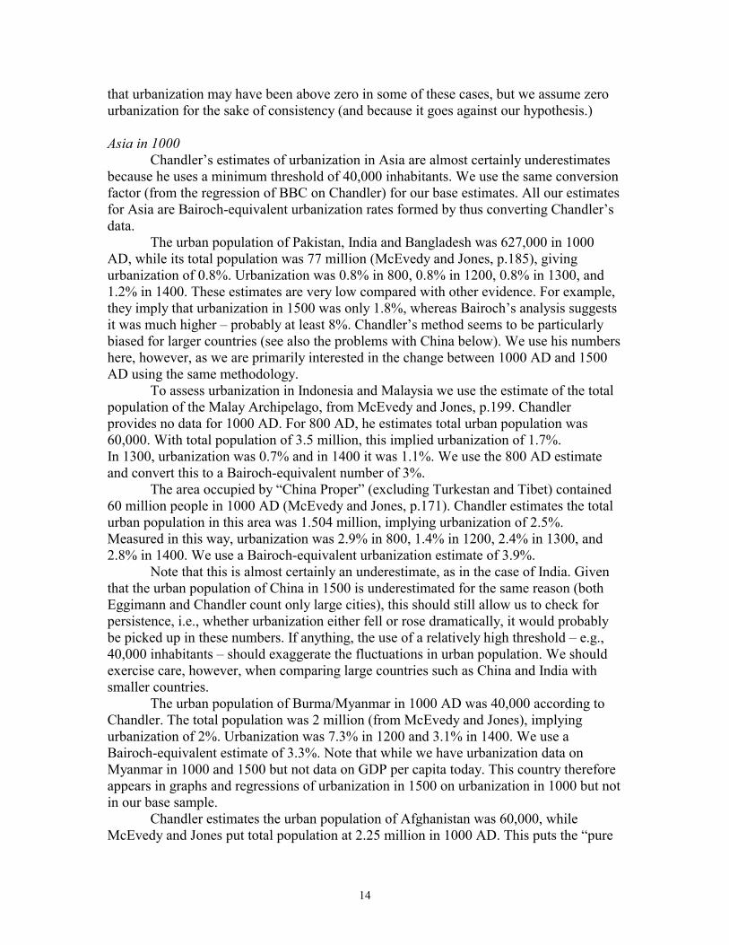
14
that urbanization may have been above zero in some of these cases, but we assume zero urbanization for the sake of consistency (and because it goes against our hypothesis.) Asia in 1000
Chandler’s estimates of urbanization in Asia are almost certainly underestimates because he uses a minimum threshold of 40,000 inhabitants. We use the same conversion factor (from the regression of BBC on Chandler) for our base estimates. All our estimates for Asia are Bairoch-equivalent urbanization rates formed by thus converting Chandler’s data. The urban population of Pakistan, India and Bangladesh was 627,000 in 1000 AD, while its total population was 77 million (McEvedy and Jones, p.185), giving urbanization of 0.8%. Urbanization was 0.8% in 800, 0.8% in 1200, 0.8% in 1300, and 1.2% in 1400. These estimates are very low compared with other evidence. For example, they imply that urbanization in 1500 was only 1.8%, whereas Bairoch’s analysis suggests it was much higher – probably at least 8%. Chandler’s method seems to be particularly biased for larger countries (see also the problems with China below). We use his numbers here, however, as we are primarily interested in the change between 1000 AD and 1500 AD using the same methodology. To assess urbanization in Indonesia and Malaysia we use the estimate of the total population of the Malay Archipelago, from McEvedy and Jones, p.199. Chandler provides no data for 1000 AD. For 800 AD, he estimates total urban population was 60,000. With total population of 3.5 million, this implied urbanization of 1.7%. In 1300, urbanization was 0.7% and in 1400 it was 1.1%. We use the 800 AD estimate and convert this to a Bairoch-equivalent number of 3%.
The area occupied by “China Proper” (excluding Turkestan and Tibet) contained 60 million people in 1000 AD (McEvedy and Jones, p.171). Chandler estimates the total urban population in this area was 1.504 million, implying urbanization of 2.5%. Measured in this way, urbanization was 2.9% in 800, 1.4% in 1200, 2.4% in 1300, and 2.8% in 1400. We use a Bairoch-equivalent urbanization estimate of 3.9%.
Note that this is almost certainly an underestimate, as in the case of India. Given that the urban population of China in 1500 is underestimated for the same reason (both Eggimann and Chandler count only large cities), this should still allow us to check for persistence, i.e., whether urbanization either fell or rose dramatically, it would probably be picked up in these numbers. If anything, the use of a relatively high threshold – e.g., 40,000 inhabitants – should exaggerate the fluctuations in urban population. We should exercise care, however, when comparing large countries such as China and India with smaller countries.
The urban population of Burma/Myanmar in 1000 AD was 40,000 according to Chandler. The total population was 2 million (from McEvedy and Jones), implying urbanization of 2%. Urbanization was 7.3% in 1200 and 3.1% in 1400. We use a Bairoch-equivalent estimate of 3.3%. Note that while we have urbanization data on Myanmar in 1000 and 1500 but not data on GDP per capita today. This country therefore appears in graphs and regressions of urbanization in 1500 on urbanization in 1000 but not in our base sample. Chandler estimates the urban population of Afghanistan was 60,000, while McEvedy and Jones put total population at 2.25 million in 1000 AD. This puts the “pure

15
Chandler” urbanization estimate at 2.7% and we use a Bairoch-equivalent estimate of 4.1%. No other information on urbanization before 1500 is available. Urbanization in Sri Lanka was 7.5% in 1200 – urban population of 75,000 from Chandler and total population of 1 million from McEvedy and Jones. No other data on urbanization before 1500 are available. We treat this as missing data for 1000 AD. We have no data on urbanization in Vietnam until 1300. At that date, the urban population, according to Chandler was 40,000. McEvedy and Jones’ total population estimate of 1 million implies an urbanization estimate of 4%. We treat this as missing data for 1000 AD.
We have no data on urbanization in the Philippines on or around 1000 AD. We have no information about urbanization in Laos in or around 1000 AD. We treat this as missing data for 1000 AD.
We assume urbanization in Hong Kong and Singapore was 3% in 1000, following the same reasoning as in our previous appendix on 1500. The Pacific Region in 1000
We assume zero urbanization in 1000 for Australia, New Zealand. This does not seem controversial. There is no sign of significant urban structures in Australia before 1800. In New Zealand, there may have been some very small-scale urbanization, but even if we increased the urbanization estimate to 3% (as for 1500), this would not change any of our results.
Africa in 1000 As is the case for 1500, the data on North Africa is reasonable and probably not subject to greater error than other non-European data. We have information on urbanization in 1000 for all North African countries, except Libya.
For Egypt in 1000, Chandler reports an urban population of 285,000. McEvedy and Jones estimate the total population was 5 million at this date, implying urbanization of 5.7%. Urbanization, calculated from these sources, was 3.9% in 800, 10.6% in 1200, 13.5% in 1300, and 14.5% in 1400. We use a Bairoch-equivalent estimate of 7.5%. For Tunisia, Chandler puts the urban population in 1000 at 60,000 and McEvedy and Jones estimate total population was 1 million. We convert this estimate of urbanization, 6%, into a Bairoch-equivalent estimate of 7.8%. Urbanization, in Chandler’s units, was 12.5% in 800, 6% in 1200, 7% in 1300 and 8.8% in 1400.
Chandler estimates the urban population of Algeria was 20,000 in 1000 AD. McEvedy and Jones put total population at 2 million, implying urbanization of 1%. Urbanization was 1.6% in 800, 2% in 1200, 7% in 1300 and 9.1% in 1400. We use a Bairoch-equivalent estimate of 2.2%. For Morocco, McEvedy and Jones put total population in 1000 at 2 million and Chandler puts the urban population at 100,000, implying urbanization of 5%. The same combination of sources gives urbanization of 3.25% in 800, 23% in 1200, 17.3% in 1300, and 14.8% in 1400. We use a Bairoch-equivalent estimate of 6.7%. As previously discussed, the data on urbanization in sub-Saharan Africa are fragmentary, of dubious value and almost certainly underestimates true urbanization with biases that are hard to assess. The data for 1000 AD are worse than for 1500 and we do not use it in our analysis.

Table 1Descriptive Statistics
Whole World
Base Sample for population
density
Base Sample for
urbanization
Below median population density in
1500
Above median population
density in 1500
Below median
urbanization in 1500
Above median
urbanization in 1500
(1) (2) (3) (4) (5) (6) (7)
Log GDP per capita (PPP) in 1995 8.3 7.9 8.5 8.3 7.5 8.8 8.1(1.1) (1.0) (0.9)
Log Population Density in 1500 1.0 0.5 0.2 -0.6 1.6 -0.9 1.4(1.6) (1.5) (1.9)
Population Density in 1500 9.2 4.8 6.3 0.8 9.1 1.2 11.7(24.3) (11.7) (16.4)
Log Population Density in 1000 0.6 0.08 0.11 -0.94 1.04 -1.20 1.22(1.5) (1.5) (2.0)
Urbanization in 1995 53.0 45.4 57.5 53.5 36.7 64.9 49.7(23.8) (22.2) (22.4)
Urbanization in 1700 8.1 5.9 6.7 2.8 4.5 2.8 10.4(8.7) (5.1) (5.6)
Urbanization in 1500 7.3 6.4 6.4 2.3 9.5 2.4 10.5(5.0) (5.0) (5.0)
Urbanization in 1000 4.7 4.0 4.0 0.8 6.7 0.8 6.4(4.4) (3.9) (3.9)
Average Protection Against Expropriation, 7.1 6.5 6.9 6.8 6.2 7.5 6.3 1985-95 (1.8) (1.4) (1.5)Constraint on the Executive in 1990 3.6 3.7 4.9 4.0 3.5 5.1 4.6
(2.3) (2.3) (2.1)Constraint on the Executive in 1900 1.9 2 2.7 2.2 1.7 3.0 2.4
(1.8) (1.9) (2.3)Constraint on the Executive in 3.6 3.4 3.3 3.6 3.3 3.8 2.8First Year of Independence (2.4) (2.3) (2.5)
Number of Observations 162 91 41 47 44 21 20
Standard deviations are in parentheses. Number of observations varies across rows due to missing data. The first 3 columns report mean values for the sample indicated at the head of the column. The last 4 columns report mean values for countries below and above the median, separately for the base urbanization and population density samples. For detailed sources and descriptions see Appendix Table A1.

Table 2Urbanization and Per Capita Income
Cross-sectional regression in 1900, all countries
Cross-sectional regression in 1950, all countries
Cross-sectional regression in 1995, all countries
Cross-sectional regression in 1995, only
for excolonies
Cross-sectional regression in 1995,
never colonized countries only
Cross-sectional regression in 1995, all
countries, with continent dummies
(1) (2) (3) (4) (5) (6)
Urbanization 0.038 0.026 0.036 0.037 0.033 0.030(0.006) (0.002) (0.002) (0.003) (0.007) (0.002)
R-Squared 0.69 0.57 0.63 0.69 0.34 0.68Number of Observations 22 128 162 93 51 162
Using panel data set through 1900
Using panel data set through 1900
Using panel data set through 1900
Using panel data set through 1900
(7) (8) (9) (10)
Urbanization 0.034 0.030 0.041 0.026(0.004) (0.004) (0.004) (0.004)
Country Dummies No No Yes Yes
Period Dummies No Yes No Yes
R-Squared 0.52 0.71 0.87 0.96Number of Observations 62 62 62 62
Panel B: Dependent Variable is Log GDP per capita
Log GDP per capita through 1900 is from Bairoch (1978), with the addition of Gregory King for England before 1700, from Snooks (1994). Urbanization is percent of population living in towns with at least 5,000 people, from Bairoch (1988) through 1900 with supplementary sources as described in the appendix. Log GDP per capita in 1950 is from Maddison (1995); this regression uses urbanization in 1960 from the World Bank's World Development Indicators 1999. Log GDP per capita (PPP) and Urbanization data for 1995 are from the World Bank's World Development Indicators 1999. Population density is total population divided by arable land area, both from McEvedy and Jones (1978). For detailed sources and descriptions see Appendix Table A1.
Panel A: Dependent Variable is Log GDP per capita
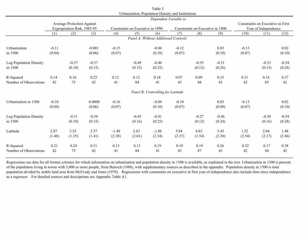
Table 3Urbanization, Population Density and Institutions
(1) (2) (3) (4) (5) (6) (7) (8) (9) (10) (11) (12)Panel A: Without Additional Controls
Urbanization -0.11 -0.001 -0.15 -0.04 -0.12 0.03 -0.13 0.02in 1500 (0.04) (0.06) (0.07) (0.10) (0.07) (0.10) (0.07) (0.10)
Log Population Density -0.37 -0.37 -0.49 -0.40 -0.35 -0.51 -0.33 -0.54in 1500 (0.10) (0.15) (0.15) (0.25) (0.12) (0.26) (0.15) (0.28)
R-Squared 0.14 0.16 0.25 0.12 0.12 0.18 0.07 0.09 0.15 0.31 0.16 0.37Number of Observations 42 75 42 41 84 41 43 88 43 42 85 42
Panel B: Controlling for Latitude
Urbanization in 1500 -0.10 -0.0008 -0.16 -0.04 -0.10 0.03 -0.13 0.02(0.04) (0.06) (0.07) (0.10) (0.07) (0.09) (0.07) (0.10)
Log Population Density -0.31 -0.34 -0.45 -0.41 -0.27 -0.46 -0.30 -0.54in 1500 (0.10) (0.15) (0.16) (0.25) (0.12) (0.24) (0.16) (0.28)
Latitude 2.87 3.53 2.57 -1.49 2.63 -1.86 5.84 4.83 5.45 1.52 2.68 1.48(1.48) (1.25) (1.41) (2.38) (2.01) (2.34) (2.37) (1.54) (2.30) (2.54) (2.17) (2.46)
R-Squared 0.21 0.24 0.31 0.13 0.13 0.19 0.19 0.19 0.26 0.32 0.17 0.38Number of Observations 42 75 42 41 84 41 43 87 43 42 84 42
Constraints on Executive in First Year of Independence
Regressions use data for all former colonies for which information on urbanization and population density in 1500 is available, as explained in the text. Urbanization in 1500 is percent of the population living in towns with 5,000 or more people, from Bairoch (1988), with supplementary sources as described in the appendix. Population density in 1500 is total population divided by arable land area from McEvedy and Jones (1978). Regressions with constraints on executive in first year of independence also include time since independence as a regressor. For detailed sources and descriptions see Appendix Table A1.
Dependent Variable is:Average Protection Against Expropriation Risk, 1985-95 Constraints on Executive in 1990 Constraints on Executive in 1900

Table 4Urbanization in 1500 and GDP per capita in 1995 for former European colonies
base samplewithout North
Africawithout the Americas
just the Americas
with continent dummies
without neo-Europes
controlling for latitude
controlling for other
geography controlling for colonial origin
controlling for religion
(1) (2) (3) (4) (5) (6) (7) (8) (9) (10)Urbanization in 1500 -0.08 -0.10 -0.12 -0.05 -0.08 -0.05 -0.07 -0.09 -0.07 -0.06
(0.03) (0.03) (0.05) (0.03) (0.03) (0.03) (0.03) (0.04) (0.03) (0.03)Asia Dummy -1.33
(0.61)Africa Dummy -0.53
(0.77)America Dummy -0.96
(0.57)Former French Colony -0.59
(0.39)Former Spanish Colony 0.06
(0.29)P-Value for Temperature [0.23]P-Value for Humidity [0.67]P-Value for Soil Quality [0.95]P-Value for Natural Resources [0.92]Dummy for Landlocked -1.14
(0.63)Latitude 1.42
(0.92)P-value for Religion [0.47]
R-Squared 0.19 0.22 0.26 0.13 0.32 0.09 0.24 0.62 0.27 0.25Number of Observations 41 37 17 24 41 37 41 41 41 41
Dependent Variable is log GDP per capita (PPP basis) in 1995. Base sample is all former colonies for which we have data. Urbanization in 1500 is percent of the population living in towns with 5,000 or more people. The regression that includes continent dummies omits Oceania. The neo-Europes are the USA, Canada, Australia and New Zealand. In the "other geography" regression we include 5 measures of temperature, 4 measures of humidity, 7 measures of soil quality, and 5 measures of natural resources. The regression that controls for colonial origin includes dummies for former French colony, Spanish colony, Portuguese colony, Belgian colony, Italian colony, German colony, and Dutch colony. British colonies are omitted. The religion variables are percent of the population who are Muslim, Catholic, and "other"; percent Protestant is omitted. For detailed sources and descriptions see Appendix Table A1.
Dependent Variable is log GDP per capita (PPP basis) in 1995
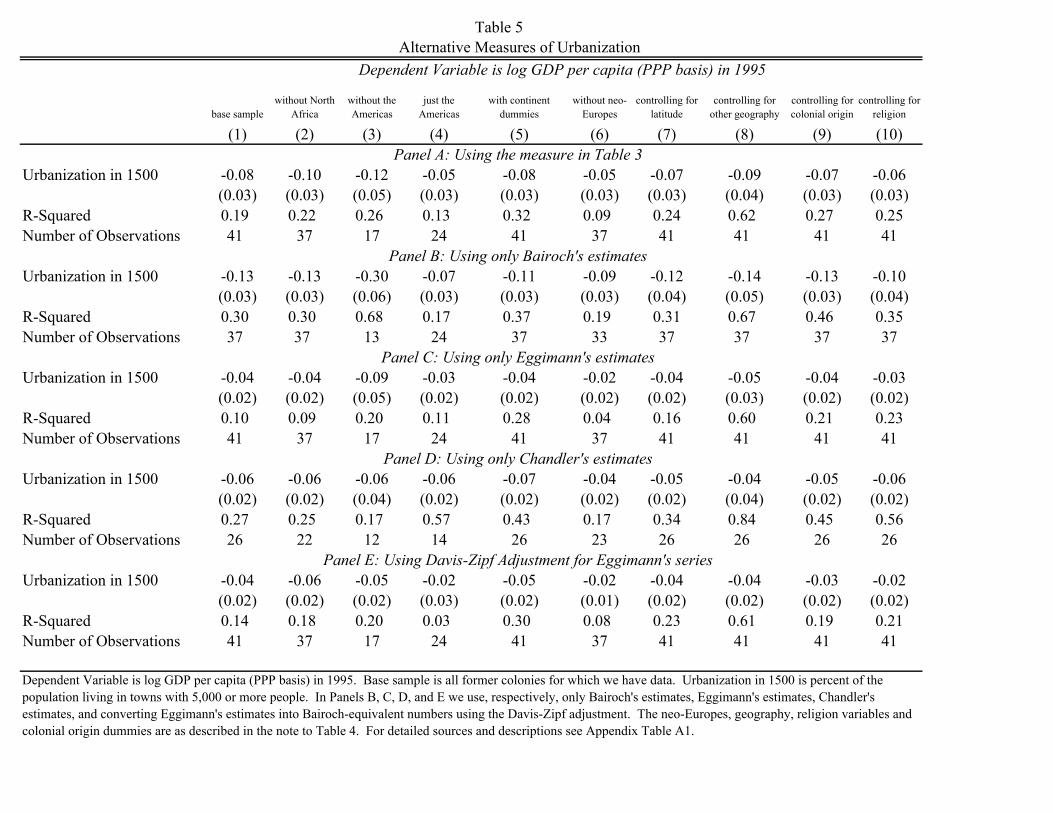
Table 5Alternative Measures of Urbanization
base samplewithout North
Africawithout the Americas
just the Americas
with continent dummies
without neo-Europes
controlling for latitude
controlling for other geography
controlling for colonial origin
controlling for religion
(1) (2) (3) (4) (5) (6) (7) (8) (9) (10)Panel A: Using the measure in Table 3
Urbanization in 1500 -0.08 -0.10 -0.12 -0.05 -0.08 -0.05 -0.07 -0.09 -0.07 -0.06(0.03) (0.03) (0.05) (0.03) (0.03) (0.03) (0.03) (0.04) (0.03) (0.03)
R-Squared 0.19 0.22 0.26 0.13 0.32 0.09 0.24 0.62 0.27 0.25Number of Observations 41 37 17 24 41 37 41 41 41 41
Panel B: Using only Bairoch's estimatesUrbanization in 1500 -0.13 -0.13 -0.30 -0.07 -0.11 -0.09 -0.12 -0.14 -0.13 -0.10
(0.03) (0.03) (0.06) (0.03) (0.03) (0.03) (0.04) (0.05) (0.03) (0.04)R-Squared 0.30 0.30 0.68 0.17 0.37 0.19 0.31 0.67 0.46 0.35Number of Observations 37 37 13 24 37 33 37 37 37 37
Panel C: Using only Eggimann's estimatesUrbanization in 1500 -0.04 -0.04 -0.09 -0.03 -0.04 -0.02 -0.04 -0.05 -0.04 -0.03
(0.02) (0.02) (0.05) (0.02) (0.02) (0.02) (0.02) (0.03) (0.02) (0.02)R-Squared 0.10 0.09 0.20 0.11 0.28 0.04 0.16 0.60 0.21 0.23Number of Observations 41 37 17 24 41 37 41 41 41 41
Panel D: Using only Chandler's estimatesUrbanization in 1500 -0.06 -0.06 -0.06 -0.06 -0.07 -0.04 -0.05 -0.04 -0.05 -0.06
(0.02) (0.02) (0.04) (0.02) (0.02) (0.02) (0.02) (0.04) (0.02) (0.02)R-Squared 0.27 0.25 0.17 0.57 0.43 0.17 0.34 0.84 0.45 0.56Number of Observations 26 22 12 14 26 23 26 26 26 26
Panel E: Using Davis-Zipf Adjustment for Eggimann's seriesUrbanization in 1500 -0.04 -0.06 -0.05 -0.02 -0.05 -0.02 -0.04 -0.04 -0.03 -0.02
(0.02) (0.02) (0.02) (0.03) (0.02) (0.01) (0.02) (0.02) (0.02) (0.02)R-Squared 0.14 0.18 0.20 0.03 0.30 0.08 0.23 0.61 0.19 0.21Number of Observations 41 37 17 24 41 37 41 41 41 41
Dependent Variable is log GDP per capita (PPP basis) in 1995. Base sample is all former colonies for which we have data. Urbanization in 1500 is percent of the population living in towns with 5,000 or more people. In Panels B, C, D, and E we use, respectively, only Bairoch's estimates, Eggimann's estimates, Chandler's estimates, and converting Eggimann's estimates into Bairoch-equivalent numbers using the Davis-Zipf adjustment. The neo-Europes, geography, religion variables and colonial origin dummies are as described in the note to Table 4. For detailed sources and descriptions see Appendix Table A1.
Dependent Variable is log GDP per capita (PPP basis) in 1995
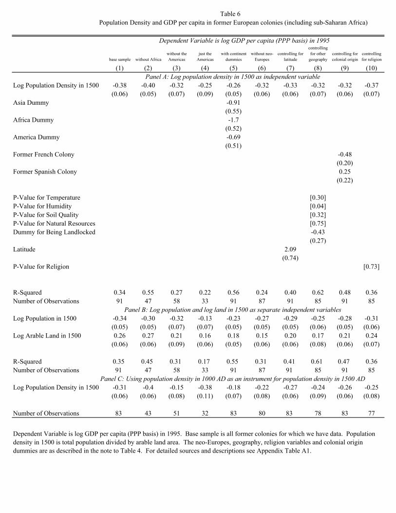
Table 6Population Density and GDP per capita in former European colonies (including sub-Saharan Africa)
base sample without Africawithout the Americas
just the Americas
with continent dummies
without neo-Europes
controlling for latitude
controlling for other
geographycontrolling for colonial origin
controlling for religion
(1) (2) (3) (4) (5) (6) (7) (8) (9) (10)Panel A: Log population density in 1500 as independent variable
Log Population Density in 1500 -0.38 -0.40 -0.32 -0.25 -0.26 -0.32 -0.33 -0.32 -0.32 -0.37(0.06) (0.05) (0.07) (0.09) (0.05) (0.06) (0.06) (0.07) (0.06) (0.07)
Asia Dummy -0.91(0.55)
Africa Dummy -1.7(0.52)
America Dummy -0.69(0.51)
Former French Colony -0.48(0.20)
Former Spanish Colony 0.25(0.22)
P-Value for Temperature [0.30]P-Value for Humidity [0.04]P-Value for Soil Quality [0.32]P-Value for Natural Resources [0.75]Dummy for Being Landlocked -0.43
(0.27)Latitude 2.09
(0.74)P-Value for Religion [0.73]
R-Squared 0.34 0.55 0.27 0.22 0.56 0.24 0.40 0.62 0.48 0.36Number of Observations 91 47 58 33 91 87 91 85 91 85
Panel B: Log population and log land in 1500 as separate independent variablesLog Population in 1500 -0.34 -0.30 -0.32 -0.13 -0.23 -0.27 -0.29 -0.25 -0.28 -0.31
(0.05) (0.05) (0.07) (0.07) (0.05) (0.05) (0.05) (0.06) (0.05) (0.06)Log Arable Land in 1500 0.26 0.27 0.21 0.16 0.18 0.15 0.20 0.17 0.21 0.24
(0.06) (0.06) (0.09) (0.06) (0.05) (0.06) (0.06) (0.08) (0.06) (0.07)
R-Squared 0.35 0.45 0.31 0.17 0.55 0.31 0.41 0.61 0.47 0.36Number of Observations 91 47 58 33 91 87 91 85 91 85
Panel C: Using population density in 1000 AD as an instrument for population density in 1500 ADLog Population Density in 1500 -0.31 -0.4 -0.15 -0.38 -0.18 -0.22 -0.27 -0.24 -0.26 -0.25
(0.06) (0.06) (0.08) (0.11) (0.07) (0.08) (0.06) (0.09) (0.06) (0.08)
Number of Observations 83 43 51 32 83 80 83 78 83 77
Dependent Variable is log GDP per capita (PPP basis) in 1995. Base sample is all former colonies for which we have data. Population density in 1500 is total population divided by arable land area. The neo-Europes, geography, religion variables and colonial origin dummies are as described in the note to Table 4. For detailed sources and descriptions see Appendix Table A1.
Dependent Variable is log GDP per capita (PPP basis) in 1995

Table 7Robustness Checks for Urbanization and Log Population Density
Base Sample
Assuming lower
urbanization in the Americas
(9% in the Andes and
Central America)
Assuming lower
urbanization in North Africa
(10%)
Assuming lower
urbanization in Indian
subcontinent (6%)
Using least favorable
combination of assumptions
Using basic Toynbee
definition of civilization (excolonies
only)
Using augmented Toynbee
definition of civilization (excolonies
only)Using land
area in 1995
Alternative assumptions
for log population
density (halve estimates for
Africa)(1) (2) (3) (4) (5) (6) (7) (8) (9)
Panel A: Unweighted RegressionsUrbanization in 1500 -0.08 -0.09 -0.10 -0.07 -0.11 -0.10 -0.12
(0.03) (0.03) (0.03) (0.03) (0.03) (0.06) (0.05)Log Population Density in 1500 -0.41 -0.32
(0.06) (0.07)R-Squared 0.20 0.22 0.24 0.16 0.21 0.45 0.30 0.35 0.21Number of Observations 41 41 41 41 41 7 14 91 91
Panel B: Regressions weighted using log population in 1500Urbanization in 1500 -0.07 -0.08 -0.10 -0.06 -0.10 -0.09 -0.12
(0.03) (0.03) (0.03) (0.03) (0.03) (0.07) (0.05)Log Population Density in 1500 -0.39 -0.29
(0.06) (0.07)R-Squared 0.18 0.22 0.23 0.14 0.20 0.27 0.29 0.32 0.19Number of Observations 41 41 41 41 41 7 14 91 91
Panel C: Including both urbanization and log population density as independent variablesUrbanization in 1500 0.04 0.04 0.02 0.04 0.02 0.07 0.07 0.02 0.003
(0.03) (0.03) (0.03) (0.03) (0.04) (0.05) (0.05) (0.02) (0.02)Log Population Density in 1500 -0.41 -0.41 -0.36 -0.40 -0.37 -0.43 -0.48 -0.43 -0.41
(0.07) (0.08) (0.07) (0.07) (0.07) (0.11) (0.10) (0.07) (0.07)R-Squared 0.56 0.56 0.54 0.56 0.54 0.85 0.79 0.61 0.60Number of Observations 41 41 41 41 41 7 14 41 41
Panel D: Instrumenting for urbanization in 1500 using log population density in 1500Urbanization in 1500 -0.18 -0.18 -0.22 -0.19 -0.24 -0.20 -0.24 -0.22 -0.24
(0.04) (0.04) (0.05) (0.05) (0.06) (0.10) (0.08) (0.05) (0.06)Number of Observations 41 41 41 41 41 7 14 41 41
Dependent Variable is log GDP per capita (PPP basis) in 1995
Dependent Variable is log GDP per capita (PPP basis) in 1995. Base sample is all former colonies for which we have data. In our base sample, urbanization in 1500 is percent of the population living in towns with 5,000 or more people. Alternative assumptions are as described at the top of each column. Population density in 1500 is total population divided by arable land area. Panel D reports the second stage coefficients from an IV regression using log population density in 1500 as the instrument. The basic Toynbee civilizations include Andean, Mexic, Yucatec, Arabic (North Africa), Hindu, Polynesian, and Eskimo (Canada). The augmented Toynbee civilizations also include North American Indian, South American Indian (Brazil/Argentina/Chile), Australian Aborigine, Malay (Malaysia and Indonesia), Philippines, Vietnam/Cambodia, and Burma. For detailed sources and descriptions see Appendix Table A1.

Table 8Persistence of Urbanization and Population Density
Base Sample Base Sample
(without Africa)
Base Sample (without America)
Base Sample (just the
Americas)
Base Sample with continent
dummies
Using augmented Toynbee definition of
civilization (excolonies only) Just Europe
All countries never colonized by
Western Europe
All countries never colonized by
Western Europe, without the Russian
Empire
All countries never colonized by
Western Europe, with continent
dummies
(1) (2) (3) (4) (5) (6) (7) (8) (9) (10)Panel A: Dependent Variable is Urbanization in 1995
Urbanization in 1500 -1.72 -2.49 -1.83 -1.24 -2.08 -2.70 1.25 1.08 1.27 1.15(0.70) (0.85) (1.40) (0.70) (0.74) (2.20) (0.40) (0.47) (0.54) (0.47)
R-Squared 0.13 0.19 0.09 0.13 0.38 0.13 0.23 0.11 0.14 0.14Number of Observations 44 39 20 24 44 12 34 46 36 46
Panel B: Dependent Variable is Urbanization in 1500Urbanization in 1000 0.96 0.88 1.49 0.95 0.89 0.82 0.46 0.42 0.46 0.45
(0.17) (0.14) (0.41) (0.14) (0.14) (0.16) (0.21) (0.17) (0.18) (0.19)R-Squared 0.50 0.57 0.53 0.68 0.73 0.73 0.14 0.13 0.17 0.14Number of Observations 35 31 14 21 35 12 31 42 35 42
Panel C: Dependent Variable is Log Population Density in 1500Log Population Density in 1000 0.91 0.97 0.86 0.92 0.83 0.82 1.15 1.06 1.13 1.03
(0.04) (0.05) (0.04) (0.09) (0.04) (0.16) (0.10) (0.06) (0.09) (0.06)R-Squared 0.88 0.89 0.90 0.78 0.90 0.70 0.83 0.85 0.79 0.85Number of Observations 88 45 55 33 88 12 33 60 44 59
Panel D: Dependent Variable is Log Population Density in 1000Log Population Density in 1 AD 0.94 1.07 0.86 1.08 0.89 0.98 0.82 0.82 0.65 0.83
(0.03) (0.02) (0.04) (0.02) (0.03) (0.23) (0.04) (0.06) (0.10) (0.06)R-Squared 0.94 0.99 0.92 0.99 0.95 0.67 0.92 0.79 0.54 0.80Number of Observations 78 44 46 32 78 11 32 55 39 54
Urbanization is the percent of the population living in cities with more than 5,000 inhabitants. Base sample is all former colonies for which we have data. Population density in 1AD, 1000 and 1500 is total population divided by arable land area. See the note to Table 7 for the list of augmented Toynbee civilizations. Column 10 includes a dummy for Asia; Europe is the omitted category. For detailed sources and descriptions see Appendix Table A1.
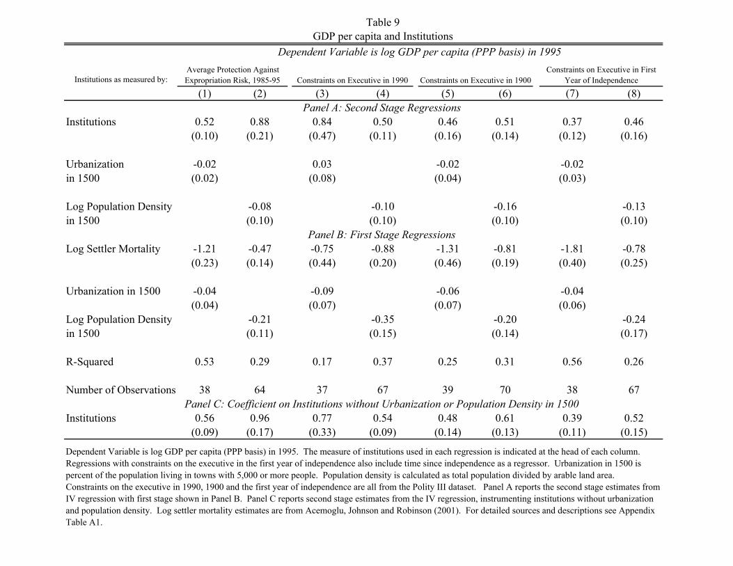
Table 9GDP per capita and Institutions
Institutions as measured by:
(1) (2) (3) (4) (5) (6) (7) (8)Panel A: Second Stage Regressions
Institutions 0.52 0.88 0.84 0.50 0.46 0.51 0.37 0.46(0.10) (0.21) (0.47) (0.11) (0.16) (0.14) (0.12) (0.16)
Urbanization -0.02 0.03 -0.02 -0.02in 1500 (0.02) (0.08) (0.04) (0.03)
Log Population Density -0.08 -0.10 -0.16 -0.13in 1500 (0.10) (0.10) (0.10) (0.10)
Panel B: First Stage RegressionsLog Settler Mortality -1.21 -0.47 -0.75 -0.88 -1.31 -0.81 -1.81 -0.78
(0.23) (0.14) (0.44) (0.20) (0.46) (0.19) (0.40) (0.25)
Urbanization in 1500 -0.04 -0.09 -0.06 -0.04(0.04) (0.07) (0.07) (0.06)
Log Population Density -0.21 -0.35 -0.20 -0.24in 1500 (0.11) (0.15) (0.14) (0.17)
R-Squared 0.53 0.29 0.17 0.37 0.25 0.31 0.56 0.26
Number of Observations 38 64 37 67 39 70 38 67Panel C: Coefficient on Institutions without Urbanization or Population Density in 1500
Institutions 0.56 0.96 0.77 0.54 0.48 0.61 0.39 0.52(0.09) (0.17) (0.33) (0.09) (0.14) (0.13) (0.11) (0.15)
Constraints on Executive in First Year of Independence
Dependent Variable is log GDP per capita (PPP basis) in 1995. The measure of institutions used in each regression is indicated at the head of each column. Regressions with constraints on the executive in the first year of independence also include time since independence as a regressor. Urbanization in 1500 is percent of the population living in towns with 5,000 or more people. Population density is calculated as total population divided by arable land area. Constraints on the executive in 1990, 1900 and the first year of independence are all from the Polity III dataset. Panel A reports the second stage estimates from IV regression with first stage shown in Panel B. Panel C reports second stage estimates from the IV regression, instrumenting institutions without urbanization and population density. Log settler mortality estimates are from Acemoglu, Johnson and Robinson (2001). For detailed sources and descriptions see Appendix Table A1.
Dependent Variable is log GDP per capita (PPP basis) in 1995Average Protection Against Expropriation Risk, 1985-95 Constraints on Executive in 1990 Constraints on Executive in 1900

Table 10The Interaction of UK Industrialization and Local Institutions
Former Colonies, using only pre-1950
data
Former Colonies, using only pre-1950
data
Former Colonies, using data through
1980 (all data)
Former Colonies, using average
institutions for each country, using only
pre-1950 data
Former Colonies, using average
institutions for each country, using all
data
Former Colonies, using average
institutions for each country,
instrumenting using settler mortality,
only pre-1950 data
Former Colonies, using average
institutions for each country,
instrumenting using settler mortality, all
data
Former Colonies, using average
institutions for each country,
instrumenting using settler mortality,
only pre-1950 data
Former Colonies, using average
institutions for each country,
instrumenting using settler mortality, all
data
All European countries, using data
through 1950
(1) (2) (3) (4) (5) (6) (7) (8) (9) (10) Panel A: Dependent Variable is Industrial Production Per Capita
UK Industrialization*Institutions 0.13 0.08 0.13 0.21 0.28 0.16 0.25 0.13 0.20 0.06(0.03) (0.03) (0.03) (0.02) (0.02) (0.03) (0.02) (0.06) (0.05) (0.01)
Institutions 8.97 9.71 -3.36 4.34(2.30) (2.58) (4.46) (0.96)
UK Industrialization*Latitude 0.30 0.52(0.49) (0.36)
R-Squared 0.75 0.44 0.74 0.87 0.94 0.85 0.94 0.83 0.93 0.78
Number of Observations 59 59 75 59 75 59 75 59 75 138
Panel B: Dependent Variable is Log GDP Per CapitaLog UK Industrialization*Institutions 0.08 0.10 0.06 0.13 0.12 0.15 0.10 0.09 0.07 0.02
(0.02) (0.05) (0.02) (0.02) (0.02) (0.03) (0.03) (0.05) (0.05) (0.01)Institutions -0.03 0.16 -0.08 -0.01
(0.03) (0.04) (0.03) (0.01)Log UK Industrialization*Latitude 0.59 0.27
(0.40) (0.38)
R-Squared 0.95 0.59 0.92 0.96 0.93 0.96 0.93 0.96 0.93 0.95
Number of Observations 79 79 131 79 131 79 131 79 131 103
Country Dummies Yes No Yes Yes Yes Yes Yes Yes Yes Yes
Period Dummies Yes Yes Yes Yes Yes Yes Yes Yes Yes Yes
Panel regressions; country and period dummies are included as indicated at the foot of each column. Dependent variable in Panel A is industrial output per capita, with up to 10 observations per country, 1750-1980, from Bairoch (1982). Dependent variable in Panel B is log GDP per capita from Maddison (1995). The independent variable of interest is total UK industrial output interacted with constraints on the executive in each country from the Polity IV dataset. The main effect of institutions is evaluated at the mean value of UK industrialization. Polity IV provides information only for independent countries; if a country was a colony at a particular date, we assign the lowest value of constraints on the executive. For detailed sources and descriptions see Appendix Table A1.

Appendix Table A1Variable Definitions and Sources
Variable Description Source
Log GDP per capita (PPP) in 1995 Logarithm of GDP per capita, on Purchasing Power Parity Basis, in 1995.World Bank, World Development Indicators, CD-Rom, 1999. Data on Surinam is from the 2000 version of this same source.
Log GDP per capita in 1900 and 1950 Logarithm of GDP per capita in 1900 and 1950.Maddison (1995) for 1950; Bairoch (1978) for 1900. In Table 10 we use data just from Maddison (1995).
Industrial Output per capita Index with Britain in 1900 equal to 100. Bairoch (1982)
Total UK industrial output Index equal to 100 in 1900. Bairoch (1982)
Log Population Density in 1 AD, 1000 and 1500 (also log population in 1500 and log arable land in 1500) Logarithm of population density (total population divided by total arable land) in 1 AD, 1000, 1500. McEvedy and Jones (1978)
Urbanization in 1960 and 1995Percent of population living in urban areas in 1960 and 1995, as defined by the UN (typically 20,000 minimum inhabitants)
World Bank, World Development Indicators, CD-Rom, 1999. For more detail, see p.159 of the World Bank's World Development Indicators 1999 (hard copy).
Urbanization in 1000, 1500, and 1700 Percent of population living in urban areas with a population of at least 5,000 in 1000, 1500, and 1700 Bairoch and supplemental sources, as described in the appendix.
European settlements in 1800 and 1900Percent of population that was European or of European descent in 1800 and 1900. Ranges from 0 to 0.99 in our base sample.
McEvedy and Jones (1978) and other sources listed in Appendix Table 5 of Acemoglu, Johnson and Robinson (2000).
Average Protection against Expropriation Risk, 1985-95Risk of expropriation of private foreign investment by government, from 0 to 10, where a higher score means less risk. We calculated the mean value for the scores in all years from 1985 to 1995.
Dataset obtained directly from Political Risk Services, September 1999. This data was previously used by Knack and Keefer (1995) and was organized in electronic form by the IRIS Center (University of Maryland). The original compilers of this data are Political Risk Services.
Constraints on Executive in 1900, 1970, 1990 and first year of independence.
A seven category scale, from 1 to 7, with a higher score indicating more constraints. Score of 1 indicates unlimited authority; score of 3 indicates slight to moderate limitations; score of 5 indicates substantial limitations; score of 7 indicates executive parity or subordination. Scores of 2, 4, and 6 indicate intermediate values.
Polity III dataset, downloaded from Inter-University Consortium for Political and Social Research. Variable described in Gurr 1997.
Percent of European descent in 1975 Percent of population that was European or of European descent in 1975. Ranges from 0 to 1 in our base sample. McEvedy and Jones (1978)
Religion Variables
Percentage of the population that belonged to the three most widely spread religions of the world in 1980 (or for 1990-95 for countries formed more recently). The classifications are: Roman Catholic, Protestant, Muslim, and "other". La Porta et al (1999)
Colonial DummiesDummy variable indicating whether country was a British, French, German, Spanish, Italian, Belgian, Dutch or Portuguese colony. La Porta et al (1999)
Temperature VariablesTemperature variables are average temperature, minimum monthly high, maximum monthly high, minimum monthly low, and maximum monthly low, all in centigrade. Parker (1997)
Humidity VariablesHumidity variables are morning minimum, morning maximum, afternoon minimum, and afternoon maximum, all in percent. Parker (1997)
Soil QualityMeasures of soil quality/climate are steppe (low latitude), desert (low latitude), steppe (middle latitude), desert (middle latitude), dry steppe wasteland, desert dry winter, and highland. Parker (1997)
Natural Resources
Measures of natural resources are: percent of world gold reserves today, percent of world iron reserves today, percent of world zinc reserves today, number of minerals present in country, and oil resources (thousands of barrels per capita.) Parker (1997)
Dummy for Landlocked Dummy variable equal to 1 if country does not adjoin the sea. Parker (1997)
Latitude Absolute value of the latitude of the country, scaled to take values between 0 and 1, where 0 is the equator. La Porta et al (1999)Log Mortality Log of estimated settler mortality. From 1.7 to 6.2. Acemoglu, Johnson and Robinson (2001)
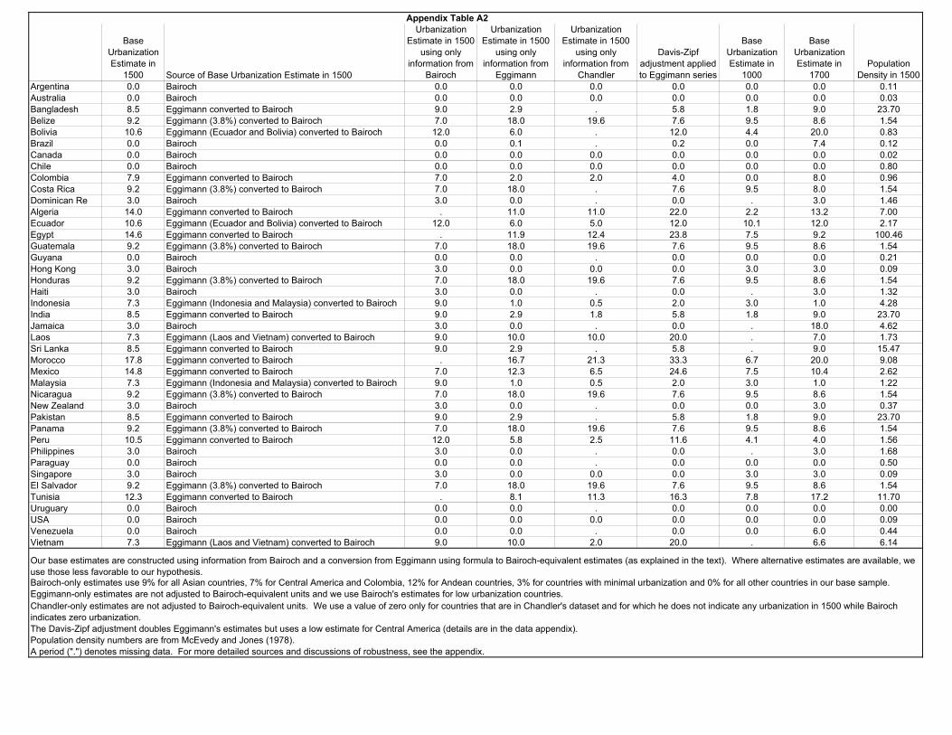
Appendix Table A2
Base Urbanization Estimate in
1500 Source of Base Urbanization Estimate in 1500
Urbanization Estimate in 1500
using only information from
Bairoch
Urbanization Estimate in 1500
using only information from
Eggimann
Urbanization Estimate in 1500
using only information from
Chandler
Davis-Zipf adjustment applied to Eggimann series
Base Urbanization Estimate in
1000
Base Urbanization Estimate in
1700Population
Density in 1500Argentina 0.0 Bairoch 0.0 0.0 0.0 0.0 0.0 0.0 0.11Australia 0.0 Bairoch 0.0 0.0 0.0 0.0 0.0 0.0 0.03Bangladesh 8.5 Eggimann converted to Bairoch 9.0 2.9 . 5.8 1.8 9.0 23.70Belize 9.2 Eggimann (3.8%) converted to Bairoch 7.0 18.0 19.6 7.6 9.5 8.6 1.54Bolivia 10.6 Eggimann (Ecuador and Bolivia) converted to Bairoch 12.0 6.0 . 12.0 4.4 20.0 0.83Brazil 0.0 Bairoch 0.0 0.1 . 0.2 0.0 7.4 0.12Canada 0.0 Bairoch 0.0 0.0 0.0 0.0 0.0 0.0 0.02Chile 0.0 Bairoch 0.0 0.0 0.0 0.0 0.0 0.0 0.80Colombia 7.9 Eggimann converted to Bairoch 7.0 2.0 2.0 4.0 0.0 8.0 0.96Costa Rica 9.2 Eggimann (3.8%) converted to Bairoch 7.0 18.0 . 7.6 9.5 8.0 1.54Dominican Re 3.0 Bairoch 3.0 0.0 . 0.0 . 3.0 1.46Algeria 14.0 Eggimann converted to Bairoch . 11.0 11.0 22.0 2.2 13.2 7.00Ecuador 10.6 Eggimann (Ecuador and Bolivia) converted to Bairoch 12.0 6.0 5.0 12.0 10.1 12.0 2.17Egypt 14.6 Eggimann converted to Bairoch . 11.9 12.4 23.8 7.5 9.2 100.46Guatemala 9.2 Eggimann (3.8%) converted to Bairoch 7.0 18.0 19.6 7.6 9.5 8.6 1.54Guyana 0.0 Bairoch 0.0 0.0 . 0.0 0.0 0.0 0.21Hong Kong 3.0 Bairoch 3.0 0.0 0.0 0.0 3.0 3.0 0.09Honduras 9.2 Eggimann (3.8%) converted to Bairoch 7.0 18.0 19.6 7.6 9.5 8.6 1.54Haiti 3.0 Bairoch 3.0 0.0 . 0.0 . 3.0 1.32Indonesia 7.3 Eggimann (Indonesia and Malaysia) converted to Bairoch 9.0 1.0 0.5 2.0 3.0 1.0 4.28India 8.5 Eggimann converted to Bairoch 9.0 2.9 1.8 5.8 1.8 9.0 23.70Jamaica 3.0 Bairoch 3.0 0.0 . 0.0 . 18.0 4.62Laos 7.3 Eggimann (Laos and Vietnam) converted to Bairoch 9.0 10.0 10.0 20.0 . 7.0 1.73Sri Lanka 8.5 Eggimann converted to Bairoch 9.0 2.9 . 5.8 . 9.0 15.47Morocco 17.8 Eggimann converted to Bairoch . 16.7 21.3 33.3 6.7 20.0 9.08Mexico 14.8 Eggimann converted to Bairoch 7.0 12.3 6.5 24.6 7.5 10.4 2.62Malaysia 7.3 Eggimann (Indonesia and Malaysia) converted to Bairoch 9.0 1.0 0.5 2.0 3.0 1.0 1.22Nicaragua 9.2 Eggimann (3.8%) converted to Bairoch 7.0 18.0 19.6 7.6 9.5 8.6 1.54New Zealand 3.0 Bairoch 3.0 0.0 . 0.0 0.0 3.0 0.37Pakistan 8.5 Eggimann converted to Bairoch 9.0 2.9 . 5.8 1.8 9.0 23.70Panama 9.2 Eggimann (3.8%) converted to Bairoch 7.0 18.0 19.6 7.6 9.5 8.6 1.54Peru 10.5 Eggimann converted to Bairoch 12.0 5.8 2.5 11.6 4.1 4.0 1.56Philippines 3.0 Bairoch 3.0 0.0 . 0.0 . 3.0 1.68Paraguay 0.0 Bairoch 0.0 0.0 . 0.0 0.0 0.0 0.50Singapore 3.0 Bairoch 3.0 0.0 0.0 0.0 3.0 3.0 0.09El Salvador 9.2 Eggimann (3.8%) converted to Bairoch 7.0 18.0 19.6 7.6 9.5 8.6 1.54Tunisia 12.3 Eggimann converted to Bairoch . 8.1 11.3 16.3 7.8 17.2 11.70Uruguary 0.0 Bairoch 0.0 0.0 . 0.0 0.0 0.0 0.00USA 0.0 Bairoch 0.0 0.0 0.0 0.0 0.0 0.0 0.09Venezuela 0.0 Bairoch 0.0 0.0 . 0.0 0.0 6.0 0.44Vietnam 7.3 Eggimann (Laos and Vietnam) converted to Bairoch 9.0 10.0 2.0 20.0 . 6.6 6.14
Eggimann-only estimates are not adjusted to Bairoch-equivalent units and we use Bairoch's estimates for low urbanization countries.
The Davis-Zipf adjustment doubles Eggimann's estimates but uses a low estimate for Central America (details are in the data appendix).Population density numbers are from McEvedy and Jones (1978).A period (".") denotes missing data. For more detailed sources and discussions of robustness, see the appendix.
Chandler-only estimates are not adjusted to Bairoch-equivalent units. We use a value of zero only for countries that are in Chandler's dataset and for which he does not indicate any urbanization in 1500 while Bairoch indicates zero urbanization.
Our base estimates are constructed using information from Bairoch and a conversion from Eggimann using formula to Bairoch-equivalent estimates (as explained in the text). Where alternative estimates are available, we use those less favorable to our hypothesis.Bairoch-only estimates use 9% for all Asian countries, 7% for Central America and Colombia, 12% for Andean countries, 3% for countries with minimal urbanization and 0% for all other countries in our base sample.
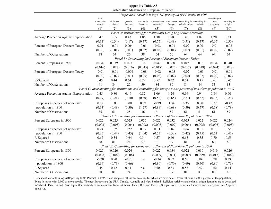
Appendix Table A3Alternative Measures of European Influence
base urbanization
sample all former colonies
just the Americas
without the Americas
with continent dummies
without neo-Europes
controlling for colonial origin
controlling for latitude
controlling for other
geography controlling for
religion
(1) (2) (3) (4) (5) (6) (7) (8) (9) (10)Panel A: Instrumenting for Institutions Using Log Settler Mortality
Average Protection Against Expropriation 0.47 1.05 0.43 1.06 1.38 1.28 1.40 1.09 1.20 1.33(0.11) (0.34) (0.17) (0.37) (0.75) (0.48) (0.51) (0.37) (0.65) (0.50)
Percent of European Descent Today 0.01 -0.01 0.004 -0.01 -0.03 -0.01 -0.02 0.00 -0.01 -0.02(0.00) (0.01) (0.01) (0.02) (0.03) (0.01) (0.02) (0.01) (0.02) (0.02)
Number of Observations 38 64 26 38 64 60 64 64 64 64Panel B: Controlling for Percent of European Descent Today
Percent Europeans in 1900 0.034 0.039 0.027 0.102 0.047 0.068 0.042 0.038 0.034 0.040(0.016) (0.017) (0.010) (0.045) (0.018) (0.023) (0.017) (0.018) (0.024) (0.018)
Percent of European Descent Today -0.01 -0.01 -0.004 -0.08 -0.02 -0.03 -0.02 -0.01 -0.01 -0.01(0.02) (0.02) (0.01) (0.05) (0.02) (0.02) (0.02) (0.02) (0.02) (0.02)
R-Squared 0.45 0.44 0.64 0.29 0.52 0.32 0.54 0.45 0.61 0.45Number of Observations 41 84 25 59 84 80 84 84 83 83
Panel C: Instrumenting for Institutions and controlling for Europeans as percent of non-slave population in 1800Average Protection Against Expropriation 0.45 0.80 0.49 0.82 1.06 1.24 0.96 0.94 0.84 0.90
(0.09) (0.21) (0.10) (0.30) (0.52) (0.65) (0.27) (0.37) (0.38) (0.23)Europeans as percent of non-slave 0.82 0.80 0.08 0.37 -0.29 1.34 0.35 0.80 1.56 -0.42 population in 1800 (0.33) (0.49) (0.30) (1.27) (0.89) (0.68) (0.59) (0.57) (0.58) (0.79)Number of Observations 35 61 25 36 61 57 61 61 61 59
Panel D: Controlling for Europeans as Percent of Non-Slave Population in 1800Percent Europeans in 1900 0.022 0.025 0.023 0.026 0.025 0.032 0.023 0.022 0.025 0.024
(0.003) (0.005) (0.004) (0.008) (0.006) (0.007) (0.004) (0.005) (0.006) (0.005)Europeans as percent of non-slave 0.24 0.76 0.22 0.35 0.31 0.82 0.64 0.81 0.70 0.58 population in 1800 (0.35) (0.44) (0.45) (1.04) (0.53) (0.53) (0.42) (0.45) (0.51) (0.47)R-Squared 0.67 0.54 0.64 0.34 0.57 0.40 0.63 0.55 0.70 0.55Number of Observations 38 81 24 57 81 77 81 81 80 80
Panel E: Controlling for Europeans as Percent of Non-Slave Population in 1800Percent Europeans in 1800 0.025 0.026 0.026 n.a. 0.022 0.034 0.022 0.019 0.019 0.026
(0.008) (0.009) (0.008) (0.009) (0.011) (0.009) (0.009) (0.012) (0.009)Europeans as percent of non-slave -0.20 0.70 -0.20 n.a. -0.34 0.57 0.60 0.84 0.78 0.39 population in 1800 (0.66) (0.73) (0.66) (0.80) (0.70) (0.69) (0.70) (0.80) (0.76)R-Squared 0.45 0.42 0.44 n.a. 0.50 0.33 0.53 0.47 0.62 0.44Number of Observations 38 81 24 n.a. 81 77 81 81 80 80
Dependent Variable is log GDP per capita (PPP basis) in 1995
Dependent Variable is log GDP per capita (PPP basis) in 1995. Base sample is all former colonies for which we have data. Urbanization in 1500 is percent of the population living in towns with 5,000 or more people. The neo-Europes are the USA, Canada, Australia and New Zealand. Religion variables and colonial origin dummies are as described in Table 4. Panels A and C use log settler mortality as an instrument for institutions. Panels B, D and E are OLS regressions. For detailed sources and descriptions see AppendixTable A1.

Log
GD
P pe
r cap
ita, P
PP, 1
995
Urbanization in 15000 5 10 15 20
7
8
9
10
ARG
AUS
BGD
BLZ
BOL
BRA
CAN
CHL
COL CRI
DOM DZAECU
EGY
GTM
GUY
HKG
HND
HTI
IDN
IND
JAM
LAO
LKA
MAR
MEXMYS
NIC
NZL
PAK
PAN
PER
PHLPRY
SGP
SLV
TUN
URY
USA
VEN
VNM
Figure 1

Figure 2Lo
g G
DP
per c
apita
, PPP
, 199
5
Log Population Density in 1500-5 0 5
6
8
10
AGO
ARG
AUS
BDI
BEN
BFA BGD
BHS
BLZ
BOL
BRA
BRB
BWA
CAF
CAN
CHL
CIVCMRCOG
COL
COM
CPV
CRI
DMADOM DZAECU
EGY
ERI
ETH
GAB
GHAGIN
GMB
GRDGTM
GUY
HKG
HND
HTI
IDN
IND
JAM
KEN
KNA
LAO
LCA
LKA
LSO
MAR
MDG
MEX
MLIMOZ
MRT
MWI
MYS
NAM
NER NGA
NIC
NPL
NZL
PAK
PAN
PER
PHLPRY
RWA
SDNSEN
SGP
SLE
SLVSUR SWZ
TCD
TGO
TTO
TUN
TZA
UGA
USA
VCT
VEN
VNM
ZAF
ZARZMB
ZWE

Figure 3Lo
g G
DP
per c
apita
, PPP
, 199
5
Urbanization in 19950 50 100
6
8
10
AGO
ARG
AUS
BDI
BEN
BFABGD
BHS
BLZ
BOL
BRA
BRB
BWA
CAF
CAN
CHL
CIVCMR COG
COL
COM
CPV
CRI
DMADOMDZAECU
EGY
ERI
ETH
FJI
GAB
GHAGIN
GMB
GRDGTM
GUY
HKG
HND
HTI
IDN
IND
JAM
KEN
KNA
LAO
LCA
LKA
LSO
MAR
MDG
MEX
MLIMOZ
MRT
MUS
MWI
MYS
NAM
NER NGA
NIC
NPL
NZL
PAK
PAN
PER
PHLPRY
RWA
SDN SEN
SGP
SLE
SLVSURSWZ
TCD
TGO
TTO
TUN
TZA
UGA
URY
USA
VCT
VEN
VNM
ZAF
ZAR ZMB
ZWE

Figure 4A Figure 4BR
esid
uals
of C
onst
rain
ts o
n Ex
ecut
ive
in F
irst Y
ear o
f Ind
epen
denc
e
Residuals of Urbanization in 1500-10 0 10
-5
0
5
ARG
AUS
BGD
BOL
BRA
CAN
CHL
COLCRIDOM
DZA
ECU
EGYGTM
GUY
HND
HTI
IDN
INDJAM
LAO
LBY
LKA
MAR
MEX
MMRMYS
NIC
NZL
PAK
PAN
PER
PHL
PNG
PRY
SGP
SLV
TUN
URY
USA
VEN
VNM
Res
idua
ls o
f Con
stra
ints
on
Exec
utiv
e in
Firs
t Yea
r of I
ndep
ende
nce
Residuals of Log Population Density in 1500-5 0 5
-5
0
5
AFGAGOARG
AUS
BDI
BENBFA
BGD
BOL
BRA
BWA
CAF
CAN
CHL
CIV
CMR
COG
COL COMCRI
CUB
DOM
DZA
ECU
EGY
ETH
GAB
GHAGIN
GMB
GNBGTM
GUY
HND
HTI
IDN
INDJAM
KENLAO
LBY
LKALSO
MAR
MDG
MEX
MLI
MMR
MOZ
MRT
MWI
MYS
NAMNER
NGA
NICNPL
NZL
PAK
PAN
PER
PHL
PNG
PRY
RWA
SDN
SEN
SGP
SLV
SOM
SWZ
TCD
TGO
TTO
TUN
TZA
UGA
URY
USA
VEN
VNM
ZAF
ZAR
ZMB
ZWE

Figure 5A Figure 5B
Log
GD
P p
er c
apita
, PP
P, 1
995
Urbanization in 17000 5 10 15 20
7
8
9
10
ARG
AUS
BGD
BLZ
BOL
BRA
CAN
CHL
COLCRI
DOM DZAECU
EGY
GTM
GUY
HKG
HND
HTI
IDN
IND
JAM
LAO
LKA
MAR
MEXMYS
NIC
NZL
PAK
PAN
PER
PHLPRY
SGP
SLV
TUN
URY
USA
VEN
VNM
Urb
aniz
atio
n in
170
0
Urbanization in 15000 5 10 15 20
0
5
10
15
20
ARGAUS
BGDBLZ
BOL
BRA
CANCHL
COL CRI
DOM
DZA
ECU
EGYGTM
GUY
HKG
HND
HTI
IDN
IND
JAM
LAO
LKA
MAR
MEX
MYS
NIC
NZL
PAKPAN
PER
PHL
PRY
SGP
SLV
TUN
URYUSA
VENVNM

Figure 6A Figure 6BUrbanization in excolonies with low and high urbanization in 1500
(averages weighted within each group by population in 1500)
0
5
10
15
20
25
800 1000 1200 1300 1400 1500 1600 1700 1750 1800 1850 1900 1920
low urbanization in 1500 excolonies high urbanization in 1500 excolonies
Urbanization in Mexico, India and USA, 800-1930(from Chandler, Mitchell and the UN)
0
10
20
30
40
50
60
70
80
90
100
800 1000 1200 1300 1400 1500 1600 1700 1750 1800 1850 1900 1920 1930
YearU
rba
niz
ati
on
(%
)
Mexico India US
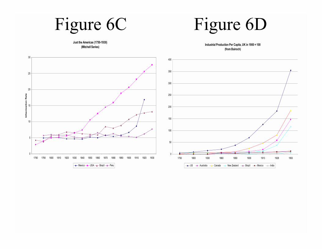
Figure 6C Figure 6DJust the Americas (1750-1930)
(Mitchell Series)
0
5
10
15
20
25
30
1750 1790 1800 1810 1820 1830 1840 1850 1860 1870 1880 1890 1900 1910 1920 1930
Urb
an
iza
tio
n R
ate
Mexico USA Brazil Peru
Industrial Production Per Capita, UK in 1900 = 100(from Bairoch)
0
50
100
150
200
250
300
350
400
1750 1800 1830 1860 1880 1900 1913 1928 1953
US Australia Canada New Zealand Brazil Mexico India
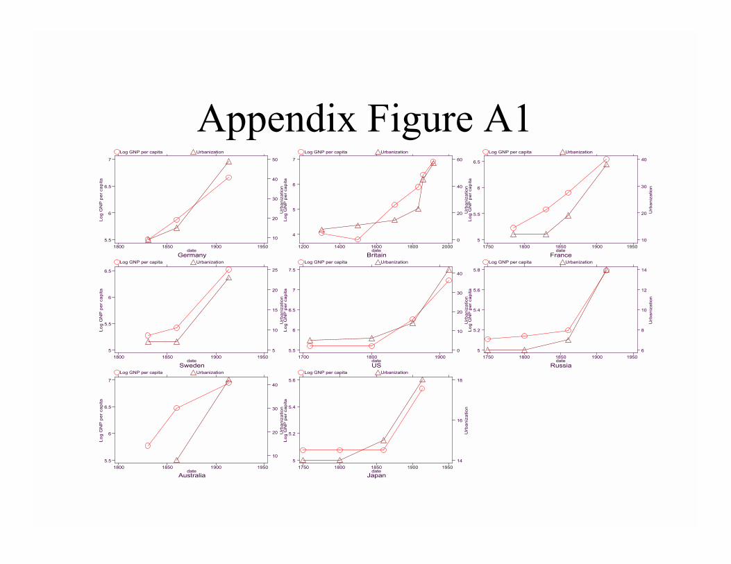
Appendix Figure A1Lo
g G
NP
per
cap
ita
Germanydate
Urb
aniz
atio
n
Log GNP per capita Urbanization
1800 1850 1900 19505.5
6
6.5
7
10
20
30
40
50
Log
GN
P p
er c
apita
Britaindate
Urb
aniz
atio
n
Log GNP per capita Urbanization
1200 1400 1600 1800 2000
4
5
6
7
0
20
40
60
Log
GN
P p
er c
apita
Francedate
Urb
aniz
atio
n
Log GNP per capita Urbanization
1750 1800 1850 1900 19505
5.5
6
6.5
10
20
30
40
Log
GN
P p
er c
apita
Swedendate
Urb
aniz
atio
n
Log GNP per capita Urbanization
1800 1850 1900 19505
5.5
6
6.5
5
10
15
20
25
Log
GN
P p
er c
apita
USdate
Urb
aniz
atio
n
Log GNP per capita Urbanization
1700 1800 19005.5
6
6.5
7
7.5
0
10
20
30
40
Log
GN
P p
er c
apita
Russiadate
Urb
aniz
atio
n
Log GNP per capita Urbanization
1750 1800 1850 1900 19505
5.2
5.4
5.6
5.8
6
8
10
12
14
Log
GN
P p
er c
apita
Australiadate
Urb
aniz
atio
n
Log GNP per capita Urbanization
1800 1850 1900 19505.5
6
6.5
7
10
20
30
40
Log
GN
P p
er c
apita
Japandate
Urb
aniz
atio
n
Log GNP per capita Urbanization
1750 1800 1850 1900 19505
5.2
5.4
5.6
14
16
18

Appendix Figure A2Lo
g G
NP
per
cap
ita
Germanydate
Log
Pop
ulat
ion
Den
sity
Log GNP per capita Log Population Density
1800 1850 1900 19505.5
6
6.5
7
4
4.5
5
Log
GN
P p
er c
apita
Britaindate
Log
Pop
ulat
ion
Den
sity
Log GNP per capita Log Population Density
1200 1400 1600 1800 2000
4
5
6
7
3
4
5
6
Log
GN
P p
er c
apita
Francedate
Log
Pop
ulat
ion
Den
sity
Log GNP per capita Log Population Density
1750 1800 1850 1900 19505
5.5
6
6.5
3.9
4
4.1
4.2
4.3
Log
GN
P p
er c
apita
Swedendate
Log
Pop
ulat
ion
Den
sity
Log GNP per capita Log Population Density
1800 1850 1900 19505
5.5
6
6.5
4.5
5
5.5
6
Log
GN
P p
er c
apita
USdate
Log
Pop
ulat
ion
Den
sity
Log GNP per capita Log Population Density
1700 1800 19005.5
6
6.5
7
7.5
-2
0
2
Log
GN
P p
er c
apita
Russiadate
Log
Pop
ulat
ion
Den
sity
Log GNP per capita Log Population Density
1750 1800 1850 1900 19505
5.2
5.4
5.6
5.8
1.5
2
2.5
3
Log
GN
P p
er c
apita
Australiadate
Log
Pop
ulat
ion
Den
sity
Log GNP per capita Log Population Density
1800 1850 1900 19505.5
6
6.5
7
-4
-3
-2
-1
0
Log
GN
P p
er c
apita
Japandate
Log
Pop
ulat
ion
Den
sity
Log GNP per capita Log Population Density
1750 1800 1850 1900 19505
5.2
5.4
5.6
6
6.2
6.4
6.6