© Machiraju/Möller Signals and Sampling Cis 782 Advanced Computer Graphics Raghu Machiraju.

© Machiraju/Möller

Signals and Sampling

Cis 782Advanced Computer Graphics

Raghu Machiraju


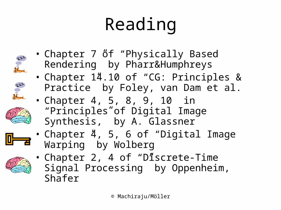
Reading

• Chapter 7 of “Physically Based Rendering” by Pharr&Humphreys

• Chapter 14.10 of “CG: Principles & Practice” by Foley, van Dam et al.

• Chapter 4, 5, 8, 9, 10 in “Principles of Digital Image Synthesis,” by A. Glassner

• Chapter 4, 5, 6 of “Digital Image Warping” by Wolberg

• Chapter 2, 4 of “Discrete-Time Signal Processing” by Oppenheim, Shafer


Motivation

• Real World - continuous

• Digital (Computer) world - discrete

• Typically we have to either:– create discrete data from continuous or (e.g.

rendering/ray-tracing, illumination models, morphing)

– manipulate discrete data (textures, surface description, image processing,tone mapping)


Motivation

• Artifacts occurring in sampling - aliasing:– Jaggies– Moire– Flickering small objects– Sparkling highlights– Temporal strobing

• Preventing these artifacts - Antialiasing


Original(continuous) signal

“manipulated”(continuous) signal

sampledsignal

“Graphics”

samplingReconstruction

filter

Motivation- Graphics


“System” orAlgorithm

Multiplication with“shah” function

Motivation

Engineering approach:

• black-box

• discretization:



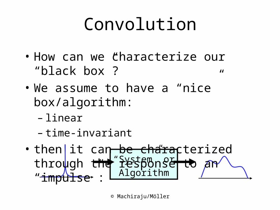
Convolution

• How can we characterize our “black box”?

• We assume to have a “nice” box/algorithm:– linear– time-invariant

• then it can be characterized through the response to an “impulse”:


• Impulse:

• discrete impulse:

• Finite Impulse Response (FIR) vs.

• Infinite Impulse Response (IIR)

1)(

0 if ,0)(

dxx

xx

1]0[

0 if ,0][

kk

Convolution (2)


• An arbitrary signal x[k] can be written as:

• Let the impulse response be h[k]:

x[k]... x[ 1][k 1] x[0][k] x[1][k 1] ...


[k] h[k]

Convolution (3)


N

Nn

nkhnxky ][][][


x[k] y[k]

IIR - N=inf.FIR - N<inf.

Convolution (4)

• for a time-invariant system h[k-n] would be the impulse response to a delayed impulse d[k-n]

• hence, if y[k] is the response of our system to the input x[k] (and we assume a linear system):


• Let’s look at a special input sequence:

• then:kiekx ][

ki

N

Nn

niki

N

Nn

nki

eH

nhee

nheky

)(

][

][][ )(

Fourier Transforms


• Hence is an eigen-function and H() its eigenvalue

• H() is the Fourier-Transform of the h[n] and hence characterizes the underlying system in terms of frequencies

• H() is periodic with period 2• H() is decomposed into

– phase (angle) response– magnitude response

kie

)(H)(H

Fourier Transforms (2)


)()()()( bGaFxbgxaf )(1)( aFaaxf

)()()()( GFxgxf )()()()( GFxgxf

)()()( Fixfdx

d nn

n

)()( Fexf i

Properties

• Linear• scaling• convolution• Multiplication

• Differentiation

• delay/shift


• Parseval’s Theorem

• preserves “Energy” - overall signal content

dFdxxf )()( 22

Properties (2)


FourierTransform

-1-0 .5

00 .5

11 .5

22 .5

33 .5

-1 0 - 8 -6 -4 -2 0 2 4 6 8 1 0

S i n c (t )

AverageFilter

-1-0 .5

00 .5

11 .5

22 .5

33 .5

-1 0 - 8 -6 -4 -2 0 2 4 6 8 1 0

S i n c (t )

Box/SincFilter

Transforms Pairs


sampling

T 1/T

Transform Pairs - Shah

• Sampling = Multiplication with a Shah function:

• multiplication in spatial domain = convolution in the frequency domain

• frequency replica of primary spectrum(also called aliased spectra)


LinearFilter

GaussianFilter

derivativeFilter

0

0 .2

0 .4

0 .6

0 .8

1

1 .2

0 0 .2 0 .6 1 1 .4 1 .8 2

linear interpolation

00.20.40.60.8

1

-6 -4 -2 0 2 4 6

00.20.40.60.8

1

-6 -4 -2 0 2 4 6

-1.5

-1

-0.5

0

0.5

1

1.5

-25 -20 -15 -10 -5 0 5 10 15 20 25

Cosc(t)

Transforms Pairs (2)


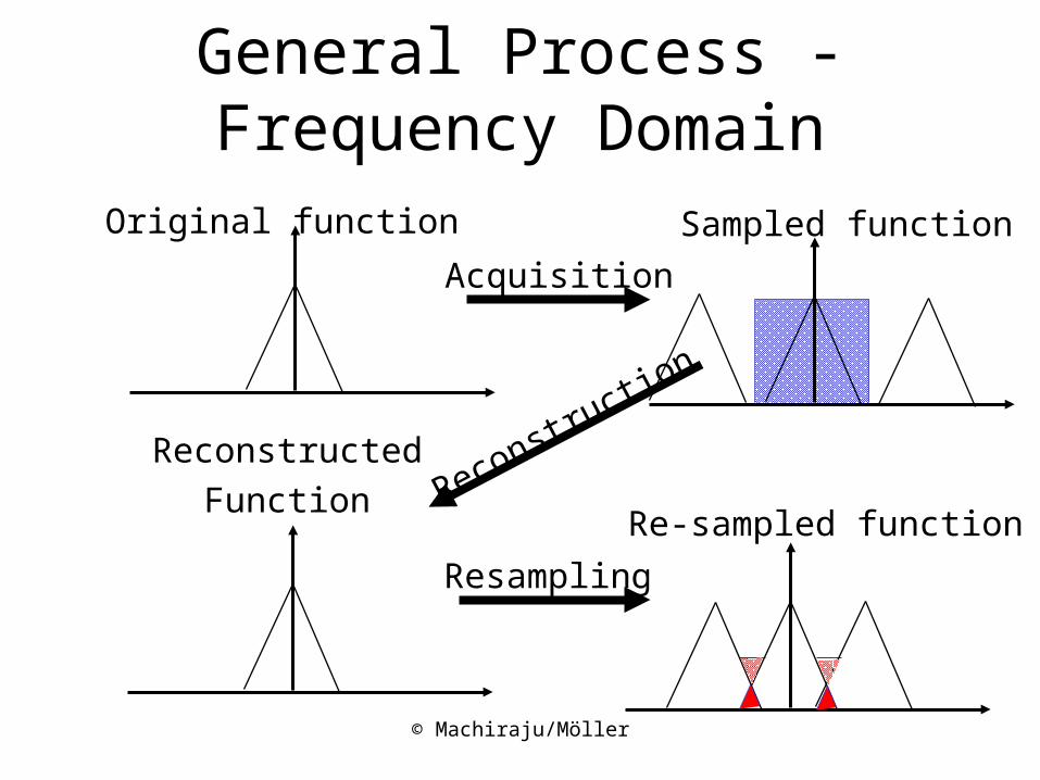
Original function Sampled function

ReconstructedFunction

Acquisition

Reconstructio

n

Re-sampled function

Resampling

General Process


Spatial Domain:

Mathematically:f(x)*h(x)

f t

h x t dt

Frequency Domain:

HF

Evaluated at discrete points (sum)

• Multiplication:• Convolution:

How? - Reconstruction

online demo

http://www.isip.msstate.edu/projects/speech/software/demonstrations/applets/util/convolution/current/


Sampling Theorem

• A signal can be reconstructed from its samples without loss of information if the original signal has no frequencies above 1/2 of the sampling frequency

• For a given bandlimited function, the rate at which it must be sampled is called the Nyquist frequency


Given

Needed

2D 1DGiven

Needed

Example


Nearest neighbor

Linear Interpolation

Example


Acquisition

Reconstructio

n

Resampling

Original function Sampled function

ReconstructedFunction

Re-sampled function

General Process -Frequency Domain


Pre-Filtering

Acquisition

Reconstruction

Original function Band-limited function

SampledFunction

Reconstructed function

Pre-Filtering


Pre-

alia

sing

Pre-filter

samplingReconstruction

filter

Post-aliasing

Once Again ...


Spatial domain Frequency domain

x

*

*

x

Pipeline - Example



x

x

*

*

Pipeline - Example (2)



x*

Pipeline - Example (3)


• Non-bandlimited signal

• Low sampling rate (below Nyquist)

• Non perfect reconstruction

Sources of Aliasing

sampling

sampling


Aliasing


Bandlimited


Spatial Domain:• convolution is exact

Frequency Domain:• cut off freq. replica

0 xfxfr x

xx

sin

Sinc

-0.4

-0.2

0

0.2

0.4

0.6

0.8

1

-25 -20 -15 -10 -5 0 5 10 15 20 250.65

0.7

0.75

0.8

0.85

0.9

0.95

0 0.05 0.1 0.15 0.2 0.25 0.3 0.35 0.4 0.45 0.5

Interpolation


0 xfxf dr

2

sincosCosc

x

x

x

xx

-1.5

-1

-0.5

0

0.5

1

1.5

-25 -20 -15 -10 -5 0 5 10 15 20 25

Cosc(t)

0.65

0.7

0.75

0.8

0.85

0.9

0.95

0 0.05 0.1 0.15 0.2 0.25 0.3 0.35 0.4 0.45 0.5

Derivatives

Spatial Domain:• convolution is exact

Frequency Domain:• cut off freq. replica


00.20.40.60.8

1

-6 -4 -2 0 2 4 60

0.20.40.60.8

1

-6 -4 -2 0 2 4 6

Spatial d. Frequency d.

Reconstruction Kernels

• Nearest Neighbor(Box)

• Linear

• Sinc

• Gaussian• Many others


Smoothing

Post-aliasing

Pass-band stop-band

Ideal filter

Practicalfilter

Ideal Reconstruction

• Box filter in frequency domain =

• Sinc Filter in spatial domain

• impossible to realize (really?)



• Use the sinc function – to bandlimit the sampled signal and remove all copies of the spectra introduced by sampling

• But:– The sinc has infinite extent and we must use

simpler filters with finite extents. – The windowed versions of sinc may introduce

ringing artifacts which are perceptually objectionable.


Reconstructing with Sinc


Low-passfilter

band-passfilter

high-passfilter


– Realizable filters do not have sharp transitions; also have ringing in pass/stop bands


T

?

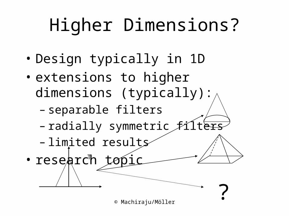
Higher Dimensions?

• Design typically in 1D

• extensions to higher dimensions (typically):– separable filters– radially symmetric filters– limited results

• research topic


Possible Errors

• Post-aliasing– reconstruction filter passes frequencies beyond the

Nyquist frequency (of duplicated frequency spectrum) => frequency components of the original signal appear in the reconstructed signal at different frequencies

• Smoothing– frequencies below the Nyquist frequency are attenuated

• Ringing (overshoot)– occurs when trying to sample/reconstruct discontinuity

• Anisotropy– caused by not spherically symmetric filters


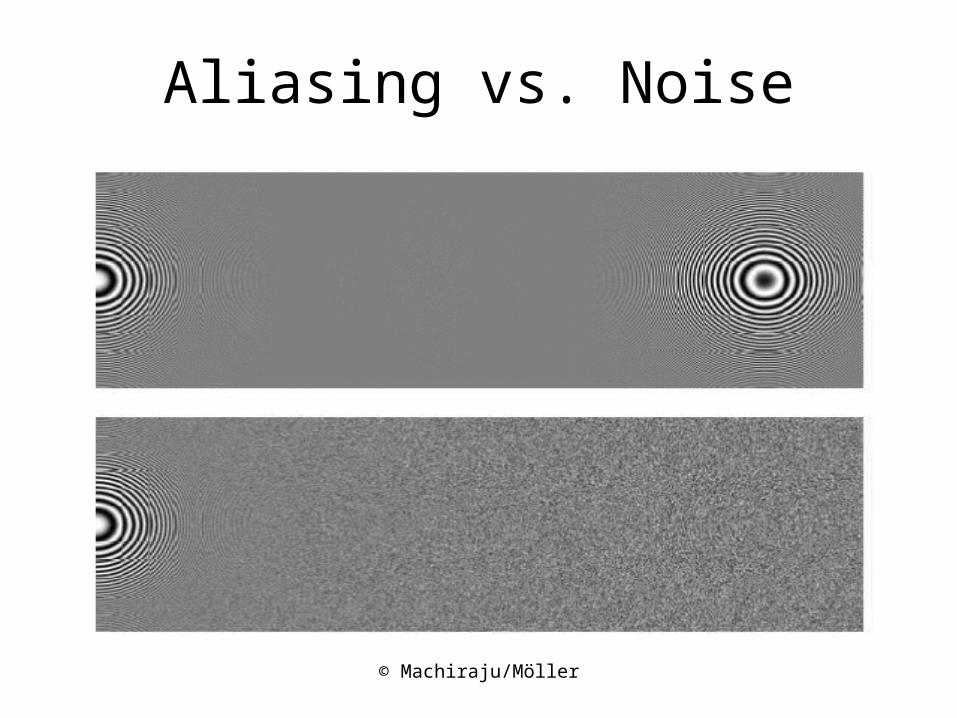
Aliasing vs. Noise


Antialiasing

• Antialiasing = Preventing aliasing

• 1. Analytically pre-filter the signal– Solvable for points, lines and polygons– Not solvable in general (e.g. procedurally

defined images)

• 2. Uniform supersampling and resample

• 3. Nonuniform or stochastic sampling


Uniform Supersampling

• Increasing the sampling rate moves each copy of the spectra further apart, potentially reducing the overlap and thus aliasing

• Resulting samples must be resampled (filtered) to image sampling rate

Pixel wk Samplek

k


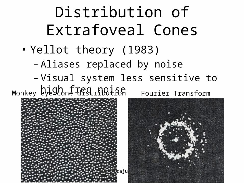
Distribution of Extrafoveal Cones

• Yellot theory (1983)– Aliases replaced by noise– Visual system less sensitive to high freq noise

Monkey eye cone distribution Fourier Transform


Non-Uniform Sampling - Intuition

• Uniform sampling– The spectrum of uniformly spaced samples is also a set of

uniformly spaced spikes– Multiplying the signal by the sampling pattern corresponds

to placing a copy of the spectrum at each spike (in freq. space)

– Aliases are coherent, and very noticeable

• Non-uniform sampling– Samples at non-uniform locations have a different

spectrum; a single spike plus noise– Sampling a signal in this way converts aliases into

broadband noise– Noise is incoherent, and much less objectionable


Non-Uniform Sampling -Patterns

• Poisson– Pick n random points in sample space

• Uniform Jitter– Subdivide sample space into n regions

• Poisson Disk– Pick n random points, but not too close


Poisson Disk Sampling

Fourier DomainSpatial Domain


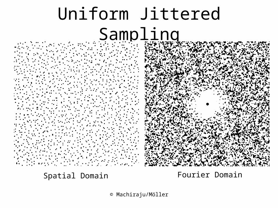
Uniform Jittered Sampling

Fourier DomainSpatial Domain


Non-Uniform Sampling - Patterns

• Spectral characteristics of these distributions:– Poisson: completely uniform (white noise).

High and low frequencies equally present– Poisson disc: Pulse at origin (DC component of

image), surrounded by empty ring (no low frequencies), surrounded by white noise

– Jitter: Approximates Poisson disc spectrum, but with a smaller empty disc.


Stratified Sampling

• Put at least one sample in each strata

• Multiple samples in strata do no good

• Also have samples far away from each other

• Graphics: jittering


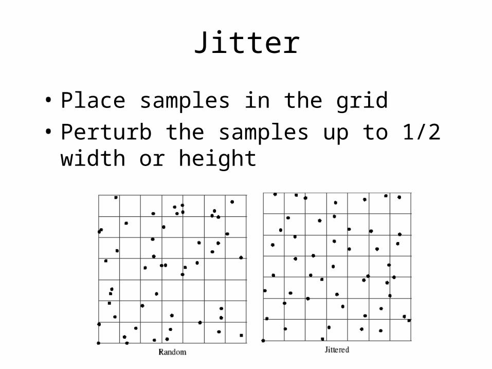
Jitter

• Place samples in the grid

• Perturb the samples up to 1/2 width or height


Exact – 256 samples/pixel Jitter with 1 sample/pixel

1 sample/pixel Jitter with 4 samples/pixel

Texture Example


Multiple Dimensions

• Too many samples

• 1D

• 2D 3D


Jitter Problems

• How to deal with higher dimensions?– Curse of dimensionality– D dimensions means ND “cells” (if we use a

separable extension)

• Solutions:– We can look at each dimension independently– We can either look in non-separable geometries– Latin Hypercube (or N-Rook) sampling


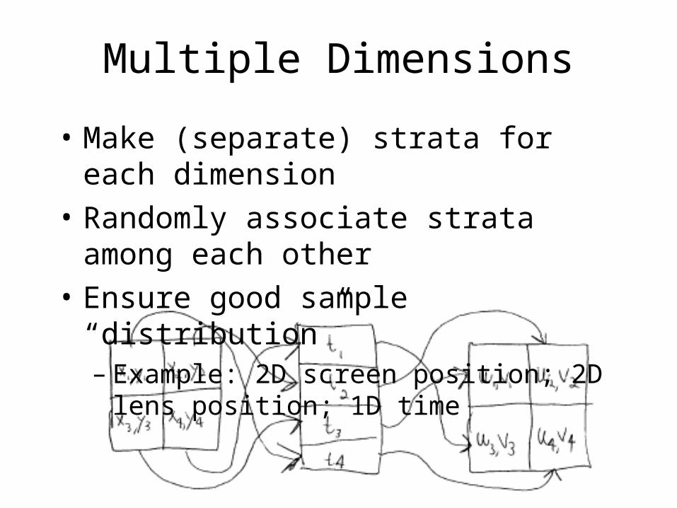
Multiple Dimensions

• Make (separate) strata for each dimension

• Randomly associate strata among each other

• Ensure good sample “distribution”– Example: 2D screen position; 2D lens position;

1D time


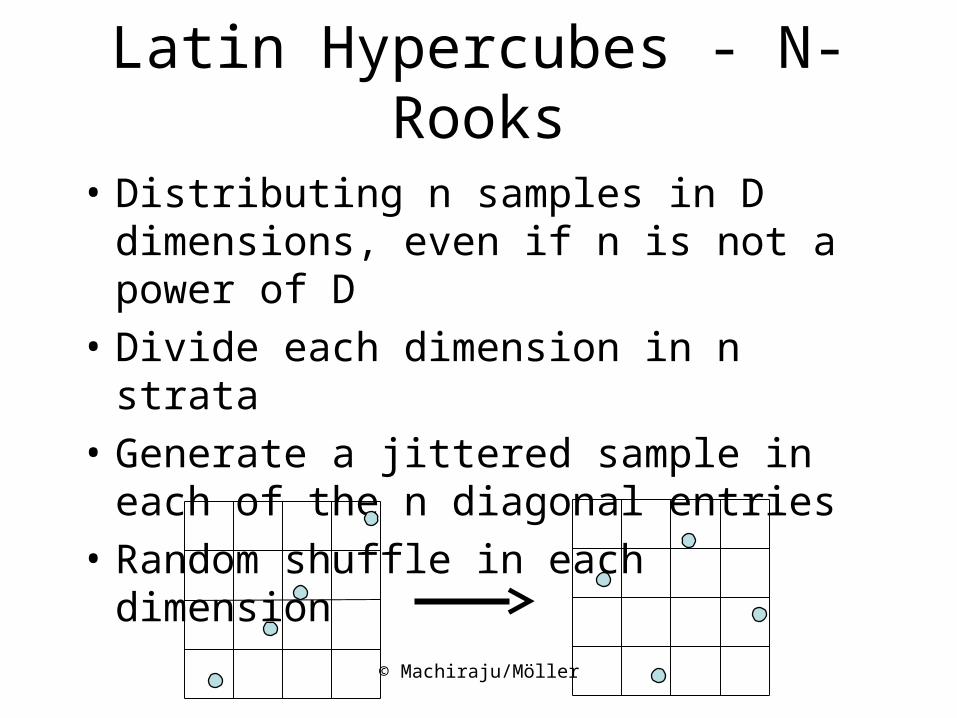
• Distributing n samples in D dimensions, even if n is not a power of D

• Divide each dimension in n strata

• Generate a jittered sample in each of the n diagonal entries

• Random shuffle in each dimension

Latin Hypercubes - N-Rooks


Stratification - problems

• Clamping (LHS helps)

• Could still have largeempty regions

• Other geometries,e.g. stratify circlesor spheres?

}


How good are the samples ?

• How can we evaluate how well our samples are distributed?– No “holes”– No clamping

• Well distributed patterns have low discrepancy– Small = evenly distributed– Large = clustering

• Construct low discrepancy sequence


V

n points

N points

Discrepancy

• DN - Maximum difference between the fraction of N points xi and relative size of volume [0,1]n

• Pick a set ofsub-volumes B of [0,1]n

• DN ->0 when N isvery large

DN B,P supbB

# x i b N

Vol b


V

n points

N points

Discrepancy

• Examples of sub-volumes B of [0,1]d:– Axis-aligned– Share a corner at the origin (star

discrepancy)

• Best discrepancy that hasbeen obtained in ddimensions:

DN* P O

logN d

N

DN* P


Discrepancy

• How to create low-discrepancy sequences?– Deterministic sequences!! Not random anymore– Also called pseudo-random– Advantage - easy to compute

• 1D:

x i i

N DN

* x1,..., xn 1

N

x i i 0.5

N DN

* x1,..., xn 1

2N

x i general DN* (x1,...,xn )

1

2Nmax

1iNx i

2i 1

2N


n ak ...a2a1 a1b0 a2b

1 a3b2 ...

b (n)0.a1a2...ak a1b 1 a2b

2 a3b 3 ...

Pseudo-Random Sequences

• Radical inverse– Building block for high-D sequences– “inverts” an integer given in base b


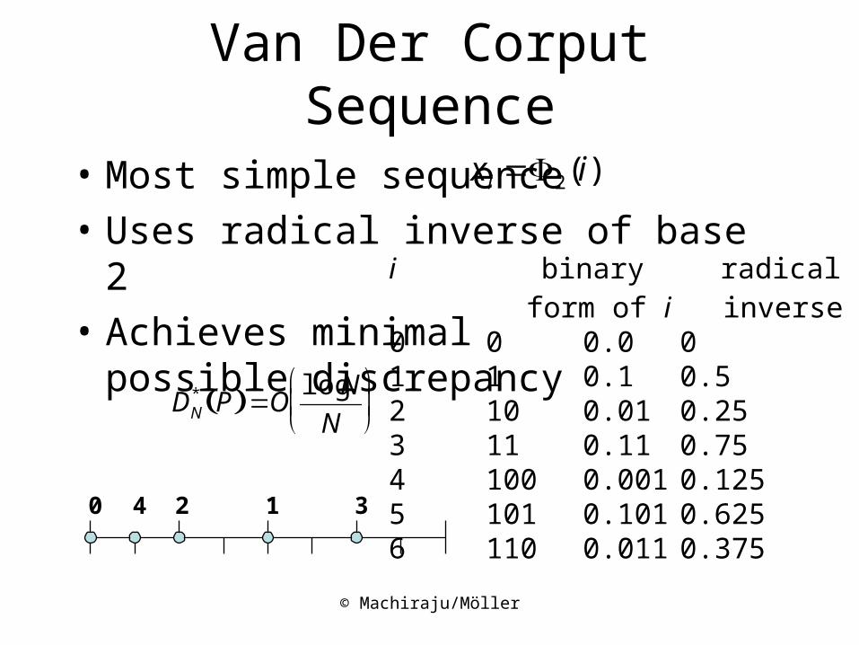
• Most simple sequence

• Uses radical inverse of base 2

• Achieves minimalpossible discrepancy

i binary radical xi

form of i inverse0 0 0.0 01 1 0.1 0.52 10 0.01 0.253 11 0.11 0.754 100 0.001 0.1255 101 0.101 0.6256 110 0.011 0.375

0 12 34

Van Der Corput Sequence

x i 2(i)

DN* P O

log N

N


x i (2(i),3(i),5(i),...,pd(i))

DN* P O

logN d

N

Halton

• Can be used if N is not known in advance

• All prefixes of a sequence are well distributed

• Use prime number bases for each dimension

• Achieves best possible discrepancy


Hammersley Sequences

x i (i 1/2

N,b1

(i),b2(i),...,bd 1

(i))

• Similar to Halton

• Need to know total number of samples in advance

• Better discrepancy than Halton


Hammersley Sequences


1

1)mod)1(()(

iiib b

bian

Folded Radical Inverse

• Hammersley-Zaremba

• Halton-Zaremba

• Improves discrepancy


Examples


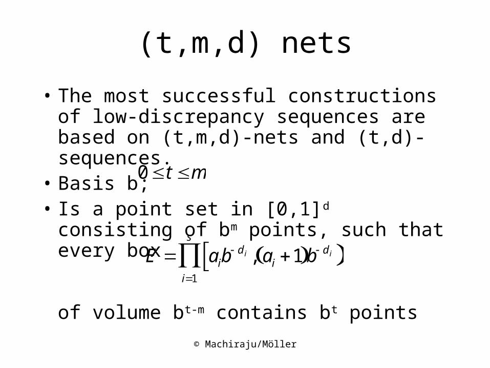
(t,m,d) nets

• The most successful constructions of low-discrepancy sequences are based on (t,m,d)-nets and (t,d)-sequences.

• Basis b; • Is a point set in [0,1]d consisting of bm

points, such that every box

of volume bt-m contains bt points

E aib d i , ai 1 b d i

i1

s

0t m


(t,d) Sequences

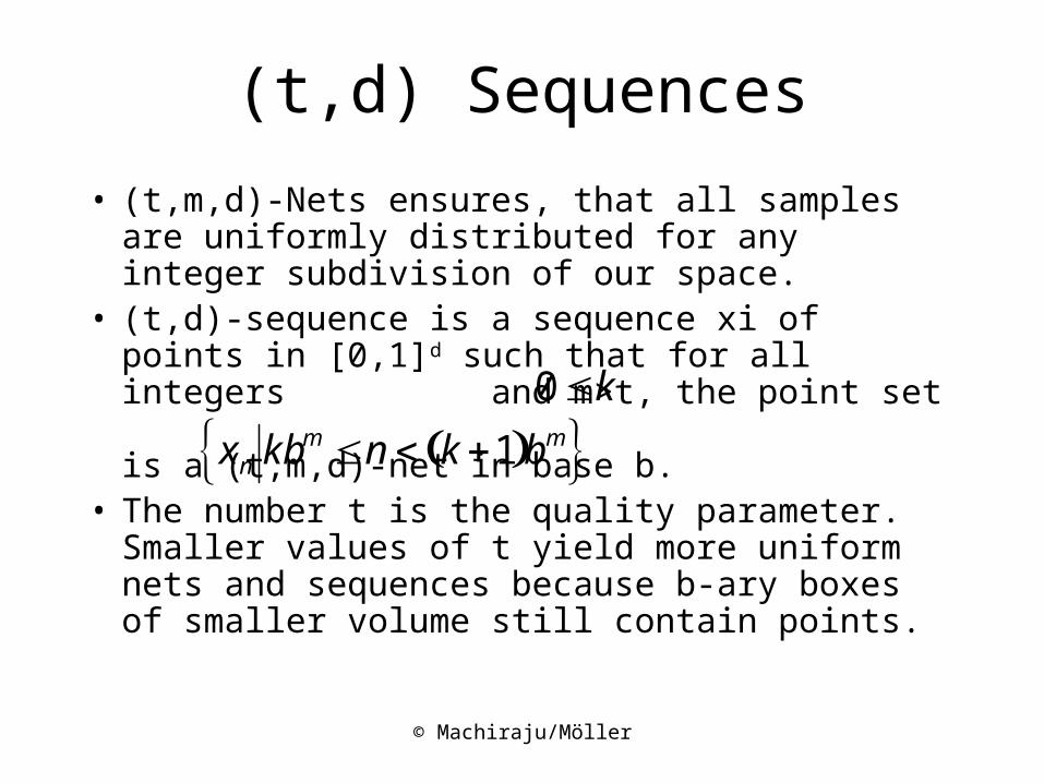
• (t,m,d)-Nets ensures, that all samples are uniformly distributed for any integer subdivision of our space.

• (t,d)-sequence is a sequence xi of points in [0,1]d such that for all integers and m>t, the point set

is a (t,m,d)-net in base b.• The number t is the quality parameter. Smaller

values of t yield more uniform nets and sequences because b-ary boxes of smaller volume still contain points.

xn kbm n k 1 bm

0k


(0,2) Sequences

• Used in pbrt for the Low-discrepancy sampler

• Base 2


Practical Issues

• Create one sequence

• Create new ones from the first sequence by “scrambling” rows and columns

• This is only possible for (0,2) sequences, since they have such a nice property (the “n-rook” property)


Texture

Jitter with 1 sample/pixel

Hammersley Sequence with 1 sample/pixel


Best-Candidate Sampling

• Jittered stratification – Randomness (inefficient)

– Clustering problems

– Undersampling (“holes”)

• Low Discrepancy Sequences– Still (visibly) aliased

• “Ideal”: Poisson disk distribution– too computationally expensive

• Best Sampling - approximation to Poisson disk


Poisson Disk

• Comes from structure of eye – rods and cones• Dart Throwing• No two points are closer than a threshold• Very expensive• Compromise – Best Candidate Sampling

– Compute pattern which is reused by tiling the image plane (translating and scaling).

– Toroidal topology– Effects the distance between points

on top to bottom



Jittered Poisson Disk Best Candidate


TextureJitter with 1 sample/pixel Best Candidate with 1 sample/pixel

Jitter with 4 sample/pixel Best Candidate with 4 sample/pixel


Next

• Probability Theory

• Monte Carlo Techniques

• Rendering Equation

© Machiraju/Möller Signals and Sampling Cis 782 Advanced Computer Graphics Raghu Machiraju.

Documents

Transcript of © Machiraju/Möller Signals and Sampling Cis 782 Advanced Computer Graphics Raghu Machiraju.