
orbilu.uni.luorbilu.uni.lu/bitstream/10993/31714/1/Linear-Algebra-2-Wiese-2017.pdf · Linear...
114
Linear Algebra 2 University of Luxembourg Gabor Wiese ∗ [email protected] Version of 7th July 2017 Contents 1 Recalls: Vector spaces, bases, dimension, homomorphisms 4 2 Recalls: Determinants 24 3 Eigenvalues 30 4 Excursion: euclidean division and gcd of polynomials 36 5 Characteristic polynmial 39 6 Minimal polynomial 44 7 Diagonalization and spectral decompostion 48 8 Jordan reduction 54 9 Hermitian spaces 67 10 Normal, adjoint, self-adjoint operators and isometries 75 11 Spectral Theorem 84 12 Quadrics 92 13 Duality 102 14 Quotients 110 ∗ translated from the French original by Luca and Massimo Notarnicola 1
Transcript of orbilu.uni.luorbilu.uni.lu/bitstream/10993/31714/1/Linear-Algebra-2-Wiese-2017.pdf · Linear...
Linear Algebra 2
University of Luxembourg
Gabor Wiese∗
Version of 7th July 2017
Contents
1 Recalls: Vector spaces, bases, dimension, homomorphisms 4
2 Recalls: Determinants 24
3 Eigenvalues 30
4 Excursion: euclidean division and gcd of polynomials 36
5 Characteristic polynmial 39
6 Minimal polynomial 44
7 Diagonalization and spectral decompostion 48
8 Jordan reduction 54
9 Hermitian spaces 67
10 Normal, adjoint, self-adjoint operators and isometries 75
11 Spectral Theorem 84
12 Quadrics 92
13 Duality 102
14 Quotients 110
∗translated from the French original by Luca and Massimo Notarnicola
1
2 CONTENTS
Preface
This is an English translation of my lecture notesAlgèbre linéaire 2, as taught in the Summer Term2017 in the academic Bachelor programme at the University of Luxembourg inthe tracks mathematicsand physics (with mathematical focus).These notes have developed over the years. They draw on various sources, most notably on Fischer’sbook Lineare Algebra(Vieweg-Verlag) and lecture notes by B. H. Matzat from the University ofHeidelberg.I would like to thank Luca and Massimo Notarnicola for taking the time to translate these notes fromFrench to English, and correcting some errors in the process.
Esch-sur-Alzette, 7 July 2017, Gabor Wiese
References
Here are some references: these books are available at the universitylibrary.
• Lelong-Ferrand, Arnaudiès.Cours de mathématiques, Tome 1, Algèbre. Dunod. Ce livre esttrès complet et très détaillé. On peut l’utiliser comme ouvrage de référence.
• Siegfried Bosch:Algebra (en allemand), Springer-Verlag. Ce livre est très complet et bienlisible.
• Serge Lang:Algebra(en anglais), Springer-Verlag. C’est comme une encyclopédie de l’algèbre;on y trouve beaucoup de sujets rassemblés, écrits de façon concise.
• Siegfried Bosch.Lineare Algebra, Springer-Verlag.
• Jens Carsten Jantzen, Joachim Schwermer.Algebra.
• Christian Karpfinger, Kurt Meyberg.Algebra: Gruppen - Ringe - Körper, Spektrum Akademis-cher Verlag.
• Gerd Fischer.Lehrbuch der Algebra: Mit lebendigen Beispielen, ausführlichen Erläuterungenund zahlreichen Bildern, Vieweg+Teubner Verlag.
• Gerd Fischer.Lineare Algebra: Eine Einführung für Studienanfänger, Vieweg+Teubner Verlag.
• Gerd Fischer, Florian Quiring.Lernbuch Lineare Algebra und Analytische Geometrie: DasWichtigste ausführlich für das Lehramts- und Bachelorstudium, Springer Vieweg.
• Perrin.Cours d’algèbre, Ellipses.
• Guin, Hausberger.Algèbre I. Groupes, corps et théorie de Galois, EDP Sciences.
• Fresnel.Algèbre des matrices, Hermann.
• Tauvel.Algèbre.
• Combes.Algèbre et géométrie.
CONTENTS 3
Prerequisites
This course contains a theoretical and a practical part. For the practicalpart, (almost) all the compu-tations can be solved by two fundamental operations:
• solving linear systems of equations,
• calculating determinants.
We are going to start the course by two sections of recalls: one about the fundaments of vector spacesand one about determinants.Linear algebra can be done over any field, not only over real or complex numbers.Some of the students may have seen the definition of a field in previous courses. For ComputerScience, finite fields, and especially the fieldF2 of two elements, are particularly important. Let usquickly recall the definition of a field.
Definition 0.1. A fieldK is a setK containing two distinct elements0, 1 and admitting two maps
+ : K ×K → K, (a, b) 7→ a+ b, “addition”
· : K ×K → K, (a, b) 7→ a · b “multiplication”,
such that for allx, y, z ∈ K, the following assertions are satisfied:
• neutral element for the addition:x+ 0 = x = 0 + x;
• associativity of the addition:(x+ y) + z = x+ (y + z);
• existence of an inverse for the multiplication:there exists an element called−x such thatx +
(−x) = 0 = (−x) + x;
• commutativity of the addition:x+ y = y + x.
• neutral element for the multiplication:x · 1 = x = 1 · x;
• associativity of the multiplication:(x · y) · z = x · (y · z);
• existence of an inverse for the multiplication:if x 6= 0, there exists an element calledx−1 = 1x
such thatx · x−1 = 1 = x−1 · x;
• commutativity for the multiplication:x · y = y · x.
• ditributivity: (x+ y) · z = x · z + y · z.
Example 0.2. • Q, R, C are fields.
• If p is a prime number,Z/pZ is a field.
• Z andN are no fields.
For the following, let K be a field. If this can help you for understanding, you can takeK = Ror K = C.
4 1 RECALLS: VECTOR SPACES, BASES, DIMENSION, HOMOMORPHISMS
1 Recalls: Vector spaces, bases, dimension, homomorphisms
Goals:
• Master the notions of vector space and subspace;
• master the notions of basis and dimension;
• master the notions of linear map ((homo)morphism), of kernel, of image;
• know examples and be able to prove simple properties.
Matrix descriptions and solving linear systems of equations by Gauss’ row reduction algorithm areassumed known and practiced.
Definition of vector spaces
Definition 1.1. LetV be a set with0V ∈ V an element, and maps
+ : V × V → V, (v1, v2) 7→ v1 + v2 = v1 + v2
(calledaddition) et
· : K × V → V, (a, v) 7→ a · v = av
(calledscalar multiplication).
We call(V,+V , ·V , 0V ) unK-vector spaceif
(A1) ∀u, v, w ∈ V : (u+V v) +V w = u+V (v +V w),
(A2) ∀ v ∈ V : 0V +V v = v = v +V 0V ,
(A3) ∀ v ∈ V ∃w ∈ V : v +V w = 0 = w +V v (we write−v := w),
(A4) ∀u, v ∈ V : u+V v = v +V u,
(for mathematicians: these properties say that(V,+V , 0V ) is an abelian group) and
(MS1) ∀ a ∈ K, ∀u, v ∈ V : a ·V (u+V v) = a ·V u+V a ·V v,
(MS2) ∀ a, b ∈ K, ∀v ∈ V : (a+K b) ·V v = a ·V v +V b ·V v,
(MS3) ∀ a, b ∈ K, ∀v ∈ V : (a ·K b) ·V v = a ·V (b ·V v),
(MS4) ∀ v ∈ V : 1 ·V v = v.
For clarity, we have written+V , ·V for the addition and the scalar multiplication inV , and+K , ·Kfor the addition and the multiplication inK. In the following, we will not do this any more.
5
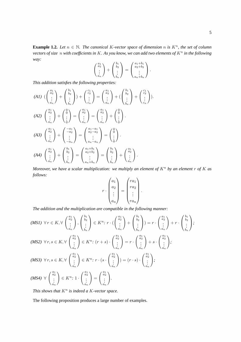
Example 1.2. Let n ∈ N. The canonicalK-vector space of dimensionn is Kn, the set of columnvectors of sizen with coefficients inK. As you know, we can add two elements ofKn in the followingway: ( a1
a2...an
)+
b1b2...bn
=
a1+b1a2+b2
...an+bn
.
This addition satisfies the following properties:
(A1) (
( a1a2...an
)+
b1b2...bn
) +
( c1c2...cn
)=
( a1a2...an
)+ (
b1b2...bn
+
( c1c2...cn
)).
(A2)
( a1a2...an
)+
( 00...0
)=
( a1a2...an
)=
( a1a2...an
)+
( 00...0
).
(A3)
( a1a2...an
)+
−a1−a2
...−an
=
a1−a1a2−a2
...an−an
=
( 00...0
).
(A4)
( a1a2...an
)+
b1b2...bn
=
a1+b1a2+b2
...an+bn
=
b1b2...bn
+
( a1a2...an
).
Moreover, we have a scalar multiplication: we multiply an element ofKn by an elementr of K asfollows:
r ·
a1a2...an
=
ra1ra2
...ran
.
The addition and the multiplication are compatible in the following manner:
(MS1) ∀ r ∈ K, ∀( a1a2...an
),
b1b2...bn
∈ Kn: r · (
( a1a2...an
)+
b1b2...bn
) = r ·
( a1a2...an
)+ r ·
b1b2...bn
;
(MS2) ∀ r, s ∈ K, ∀( a1a2...an
)∈ Kn: (r + s) ·
( a1a2...an
)= r ·
( a1a2...an
)+ s ·
( a1a2...an
);
(MS3) ∀ r, s ∈ K, ∀( a1a2...an
)∈ Kn: r · (s ·
( a1a2...an
)) = (r · s) ·
( a1a2...an
);
(MS4) ∀( a1a2...an
)∈ Kn: 1 ·
( a1a2...an
)=
( a1a2...an
).
This shows thatKn is indeed aK-vector space.
The following proposition produces a large number of examples.
6 1 RECALLS: VECTOR SPACES, BASES, DIMENSION, HOMOMORPHISMS
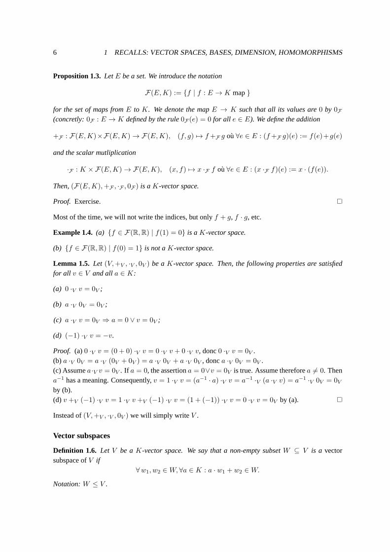
Proposition 1.3. LetE be a set. We introduce the notation
F(E,K) := {f | f : E → K map}
for the set of maps fromE to K. We denote the mapE → K such that all its values are0 by 0F(concretly:0F : E → K defined by the rule0F (e) = 0 for all e ∈ E). We define the addition
+F : F(E,K)×F(E,K) → F(E,K), (f, g) 7→ f+F g où∀e ∈ E : (f+F g)(e) := f(e)+g(e)
and the scalar mutliplication
·F : K ×F(E,K) → F(E,K), (x, f) 7→ x ·F f où∀e ∈ E : (x ·F f)(e) := x · (f(e)).
Then,(F(E,K),+F , ·F , 0F ) is aK-vector space.
Proof. Exercise.
Most of the time, we will not write the indices, but onlyf + g, f · g, etc.
Example 1.4. (a) {f ∈ F(R,R) | f(1) = 0} is aK-vector space.
(b) {f ∈ F(R,R) | f(0) = 1} is not aK-vector space.
Lemma 1.5. Let (V,+V , ·V , 0V ) be aK-vector space. Then, the following properties are satisfiedfor all v ∈ V and alla ∈ K:
(a) 0 ·V v = 0V ;
(b) a ·V 0V = 0V ;
(c) a ·V v = 0V ⇒ a = 0 ∨ v = 0V ;
(d) (−1) ·V v = −v.
Proof. (a)0 ·V v = (0 + 0) ·V v = 0 ·V v + 0 ·V v, donc0 ·V v = 0V .(b) a ·V 0V = a ·V (0V + 0V ) = a ·V 0V + a ·V 0V , donca ·V 0V = 0V .(c) Assumea·V v = 0V . If a = 0, the assertiona = 0∨v = 0V is true. Assume thereforea 6= 0. Thena−1 has a meaning. Consequently,v = 1 ·V v = (a−1 · a) ·V v = a−1 ·V (a ·V v) = a−1 ·V 0V = 0Vby (b).(d) v +V (−1) ·V v = 1 ·V v +V (−1) ·V v = (1 + (−1)) ·V v = 0 ·V v = 0V by (a).
Instead of(V,+V , ·V , 0V ) we will simply writeV .
Vector subspaces
Definition 1.6. Let V be aK-vector space. We say that a non-empty subsetW ⊆ V is a vectorsubspace ofV if
∀w1, w2 ∈W, ∀a ∈ K : a · w1 + w2 ∈W.
Notation:W ≤ V .
7
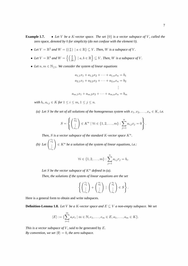
Example 1.7. • Let V be aK-vector space. The set{0} is a vector subspace ofV , called thezero space, denoted by0 for simplicity (do not confuse with the element0).
• LetV = R2 andW = {( a0 ) | a ∈ R} ⊆ V . Then,W is a subspace ofV .
• LetV = R3 andW ={(
ab2b
)| a, b ∈ R
}⊆ V . Then,W is a subspace ofV .
• Letn,m ∈ N≥1. We consider the system of linear equations
a1,1x1 + a1,2x2 + · · ·+ a1,nxn = b1
a2,1x1 + a2,2x2 + · · ·+ a2,nxn = b2
...
am,1x1 + am,2x2 + · · ·+ am,nxn = bm
with bi, ai,j ∈ K for 1 ≤ i ≤ m, 1 ≤ j ≤ n.
(a) LetS be the set of all solutions of the homogeneous system withx1, x2, . . . , xn ∈ K, i.e.
S =
( x1x2...xn
)∈ Kn | ∀i ∈ {1, 2, . . . ,m} :
n∑
j=1
ai,jxj = 0
.
Then,S is a vector subspace of the standardK-vector spaceKn.
(b) Let
( r1r2...rn
)∈ Kn be a solution of the system of linear equations, i.e.:
∀i ∈ {1, 2, . . . ,m} :n∑
j=1
ai,jrj = bi.
LetS be the vector subspace ofKn defined in (a).
Then, the solutions if the system of linear equations are the set
{( r1r2...rn
)+
( s1s2...sn
)|( s1s2...sn
)∈ S
}.
Here is a general form to obtain and write subspaces.
Definition-Lemma 1.8. LetV be aK-vector space andE ⊆ V a non-empty subspace. We set
〈E〉 := {m∑
i=1
aiei | m ∈ N, e1, . . . , em ∈ E, a1, . . . , am ∈ K}.
This is a vector subspace ofV , said to begenerated byE.
By convention, we set〈∅〉 = 0, the zero subspace.

8 1 RECALLS: VECTOR SPACES, BASES, DIMENSION, HOMOMORPHISMS
Proof. Since〈E〉 is non-empty (sinceE is non-empty), it suffizes to check the definition of subspace.Let thereforew1, w2 ∈ 〈E〉 anda ∈ K. We can write
w1 =m∑
i=1
aiei etw2 =m∑
i=1
biei
for ai, bi ∈ K andei ∈ E for all i = 1, . . . ,m. Thus we have
a · w1 + w2 =m∑
i=1
(aai + bi)ei,
which is indeed an element of〈E〉.
Example 1.9. The set{a ·(
112
)+ b ·
(007
)| a, b ∈ R
}is a subspace ofR3.
Sometimes it is useful to characterize the subspace generated by a set in a more theoretical way. Todo so, we need the following lemma.
Lemma 1.10. Let V be aK-vector space andWi ≤ V subspaces fori ∈ I 6= ∅. Then,W :=⋂i∈IWi is a vector subspace ofV .
Proof. Exercise.
In contrast,⋃i∈IWi is not a subspace in general (as you see it in an exercise)!
Example 1.11.How to compute the intersection of two subspaces?
(a) The easiest case is when the two subspaces are given as the solutionsof two systems of linearequations, for example:
• V is the subset of
( x1x2...xn
)∈ Kn such that
∑ni=1 ai,jxi = 0 for j = 1, . . . , ℓ, et
• W is the subset of
( x1x2...xn
)∈ Kn such that
∑ni=1 bi,kxi = 0 pourk = 1, . . . ,m.
In this case, the subspaceV ∩W is given as the set of common solutions for all the equalities.
(b) Suppose now that the subspaces are given as subspaces ofKn generated by finite sets of vectors:LetV = 〈E〉 andW = 〈F 〉 où
E =
e1,1e2,1...
en,1
, . . . ,
e1,me2,m
...en,m
⊆ Kn andF =
f1,1f2,1...
fn,1
, . . . ,
f1,pf2,p...
fn,p
⊆ Kn.
Then
V ∩W ={ m∑
i=1
ai
e1,ie2,i...
en,i
∣∣
∃ b1, . . . , bp ∈ K : a1
e1,1e2,1...
en,1
+ · · ·+ am
e1,me2,m
...en,m
− b1
f1,1f2,1...
fn,1
− · · · − bp
f1,pf2,p...
fn,p
= 0
}.
9
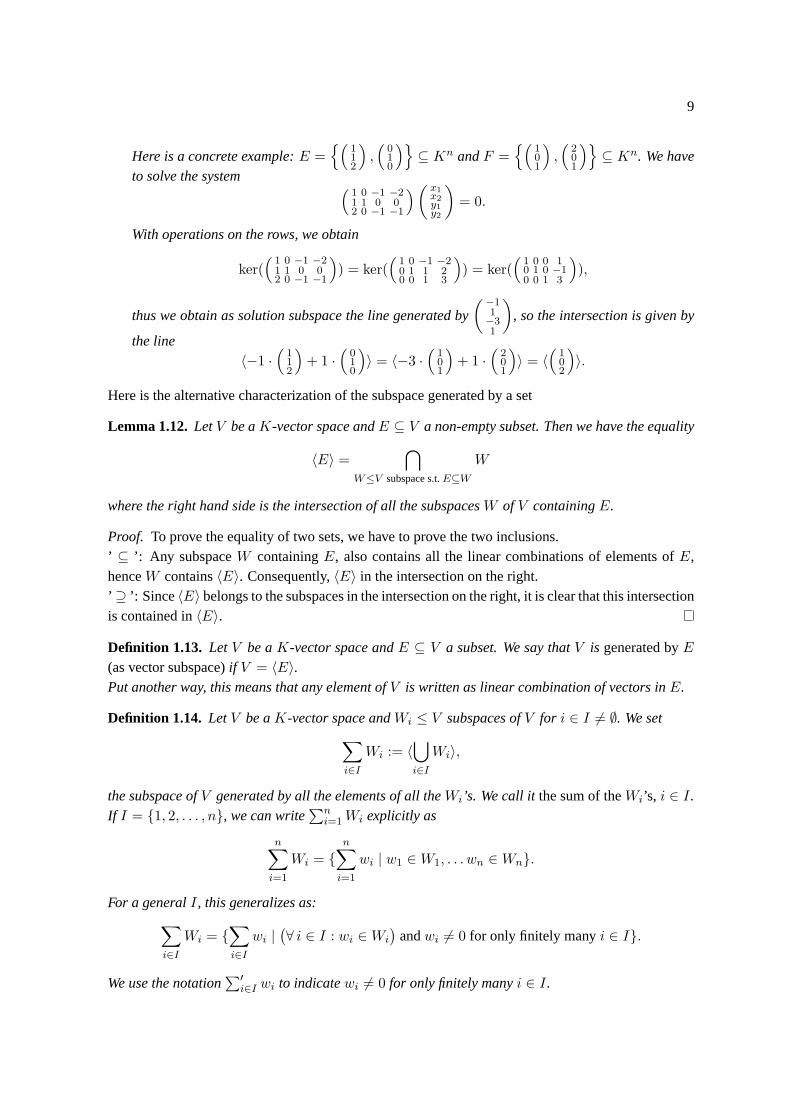
Here is a concrete example:E ={(
112
),(
010
)}⊆ Kn andF =
{(101
),(
201
)}⊆ Kn. We have
to solve the system (1 0 −1 −21 1 0 02 0 −1 −1
)( x1x2y1y2
)= 0.
With operations on the rows, we obtain
ker((
1 0 −1 −21 1 0 02 0 −1 −1
)) = ker(
(1 0 −1 −20 1 1 20 0 1 3
)) = ker(
(1 0 0 10 1 0 −10 0 1 3
)),
thus we obtain as solution subspace the line generated by
(−11−31
), so the intersection is given by
the line〈−1 ·
(112
)+ 1 ·
(010
)〉 = 〈−3 ·
(101
)+ 1 ·
(201
)〉 = 〈
(102
)〉.
Here is the alternative characterization of the subspace generated by a set
Lemma 1.12. LetV be aK-vector space andE ⊆ V a non-empty subset. Then we have the equality
〈E〉 =⋂
W≤V subspace s.t.E⊆WW
where the right hand side is the intersection of all the subspacesW of V containingE.
Proof. To prove the equality of two sets, we have to prove the two inclusions.’ ⊆ ’: Any subspaceW containingE, also contains all the linear combinations of elements ofE,henceW contains〈E〉. Consequently,〈E〉 in the intersection on the right.’ ⊇ ’: Since〈E〉 belongs to the subspaces in the intersection on the right, it is clear that this intersectionis contained in〈E〉.
Definition 1.13. LetV be aK-vector space andE ⊆ V a subset. We say thatV is generated byE(as vector subspace)if V = 〈E〉.Put another way, this means that any element ofV is written as linear combination of vectors inE.
Definition 1.14. LetV be aK-vector space andWi ≤ V subspaces ofV for i ∈ I 6= ∅. We set∑
i∈IWi := 〈
⋃
i∈IWi〉,
the subspace ofV generated by all the elements of all theWi’s. We call itthe sum of theWi’s, i ∈ I.If I = {1, 2, . . . , n}, we can write
∑ni=1Wi explicitly as
n∑
i=1
Wi = {n∑
i=1
wi | w1 ∈W1, . . . wn ∈Wn}.
For a generalI, this generalizes as:∑
i∈IWi = {
∑
i∈Iwi |
(∀ i ∈ I : wi ∈Wi
)andwi 6= 0 for only finitely manyi ∈ I}.
We use the notation∑′
i∈I wi to indicatewi 6= 0 for only finitely manyi ∈ I.
10 1 RECALLS: VECTOR SPACES, BASES, DIMENSION, HOMOMORPHISMS
Example 1.15.How to compte/obtain the sum of two subspaces?
The answer is very easy if the two subspaces are given by generators:If U = 〈E〉 andV = 〈F 〉 aresubspaces of aK-vector spaceV , thenU + V = 〈E ∪ F 〉.(The question of giving a basis for the sum is different... see later.)
When are thewi ∈Wi in the writingw =∑′
i∈I wi unique?
Definition 1.16. LetV be aK-vector space andWi ≤ V the subspace ofV for i ∈ I 6= ∅.
We say that the sumW =∑
i∈IWi is direct if for all i ∈ I we have
Wi ∩∑
j∈I\{i}Wj = 0.
Notation for direct sums:⊕
i∈IWi.
If I = {1, . . . , n}, we sometimes write the elements of a direct sum⊕n
i=1Wi asw1 ⊕w2 ⊕ · · · ⊕wn(wherewi ∈Wi for i ∈ I, of course).
Example 1.17. In Example 1.11 (b), the sumV +W is not direct since the intersectionV ∩W is aline and thus non-zero.
Proposition 1.18. Let V be aK-vector space,Wi ≤ V subspaces ofV for i ∈ I 6= ∅ andW =∑i∈IWi. Then the following assertions are equivalent:
(i) W =⊕
i∈IWi ;
(ii) for all w ∈W and all i ∈ I there exists a uniquewi ∈Wi such thatw =∑′
i∈I wi.
Proof. “(i) ⇒ (ii)”: The existence of suchwi ∈Wi is clear. Let us thus show the uniqueness
w =∑
i∈I
′wi =
∑
i∈I
′w′i
with wi, w′i ∈ Wi for all i ∈ I (remember that the notation
∑′ indicates that only finitely manywi,w′i are non-zero). This implies fori ∈ I:
wi − w′i =
∑
j∈I\{i}
′(w′
j − wj) ∈Wi ∩∑
j∈I\{i}Wj = 0.
Thus,wi − w′i = 0, sowi = w′
i for all i ∈ I, showing uniqueness.
“(ii) ⇒ (i)”: Let i ∈ I andwi ∈ Wi ∩∑
j∈I\{i}Wj . Then,wi =∑′
j∈I\{i}wj with wj ∈ Wj for allj ∈ I. We can now write0 in two ways
0 =∑
i∈I
′0 = −wi +
∑
j∈I\{i}
′wj .
Hence, the uniqueness imples−wi = 0. Therefore, we have shownWi ∩∑
j∈I\{i}Wj = 0.
11
Bases
Definition 1.19. LetV be aK-vector space andE ⊆ V a subspace.
We say thatE isK-linearly independentif
∀n ∈ N ∀ a1, . . . , an ∈ K ∀ e1, . . . , en ∈ E :( n∑
i=1
aiei = 0 ∈ V ⇒ a1 = a2 = · · · = an = 0)
(i.e., the onlyK-linear combination of elements ofE representing0 ∈ V is the one in which all thecoefficients are0). On the other hand, we say thatE isK-linearly dependent.
We callE aK-basis ofV if E generatesV andE isK-linearly independent.
Example 1.20. How to compute whether two vectors are linearly independent? (Same answer thanalmost always:) Solve a system of linear equations.
Let the subspace
e1,1e2,1...
en,1
, . . . ,
e1,me2,m
...en,m
ofKn be given. These vectors are linearly independent if and only if the only solution of the systemof linear equations
e1,1 e1,2 ... e1,me2,1 e2,2 ... e2,m...
......
...en,1 en,2 ... en,m
( x1
x2...xm
)= 0
is zero.
Example 1.21.Letd ∈ N>0. Sete1 =
100...0
, e2 =
010...0
, . . . , ed =
000...1
etE = {e1, e2, . . . , ed}.
Then:
• E generatesKd:
Any vectorv =
a1a2a3...ad
is written asK-linear combination:v =
∑di=1 aiei.
• E isK-linearly independent:
If we have aK-linear combination0 =∑d
i=1 aiei, then clearlya1 = · · · = ad = 0.
• E is thus aK-basis ofKd, sinceE generatesKd and isK-linearly independent. We call it thecanonical basisofKd.
The following theorem characterizes bases.
Theorem 1.22.LetV be aK-vector space andE = {e1, e2, . . . , en} ⊆ V be a finite subset. Then,the following assertions are equivalent:
(i) E is aK-basis.

12 1 RECALLS: VECTOR SPACES, BASES, DIMENSION, HOMOMORPHISMS
(ii) E is a minimal set of generators ofV , i.e.: E generatesV , but for all e ∈ E, the setE \ {e}does not generateV .
(iii) E is a maximalK-linearly independent set, i.e.:E is K-linearly independent, but for alle ∈V \ E, the setE ∪ {e} isK-linearly dependent.
(iv) Anyv ∈ V is written asv =∑n
i=1 aiei with uniquea1, . . . , an ∈ K.
Corollary 1.23. Let V be aK-vector space andE ⊆ V a finite set generatingV . Then,V hasK-basis contained inE.
In the appendix of this section, we will show using Zorn’s Lemma that any vector space has a basis.
Example 1.24. (a) LetV ={(
aab
)| a, b ∈ R
}. A basis ofV is
{(110
),(
001
)}.
(b) LetV = 〈(
123
),(
234
),(
357
)〉 ⊆ Q3.
The setE ={(
123
),(
234
)}is aQ-basis ofV . Reason:
• The system of linear equations
a1 ·(
123
)+ a2 ·
(234
)+ a3 ·
(357
)=(
000
)
has a non-zero solution (for instancea1 = 1, a2 = 1, a3 = −1). This imples thatEgeneratesV since we can express the third generator by the two first.
• The system of linear equations
a1 ·(
123
)+ a2 ·
(234
)=(
000
)
only hasa1 = a2 = 0 as solution. ThusE isQ-linearly independent.
(c) TheR-vectore space
V = {f : N → R | ∃S ⊆ N finite ∀n ∈ N \ S : f(n) = 0}
has{en | n ∈ N} avecen(m) = δn,m (Kronecker delta:δn,m =
{1 si n = m,
0 if n 6= m.) asR-basis.
This is thus a basis with infinitely many elements.
(d) Similarly to the previous example, theR-vector space
V = {f : R → R | ∃S ⊆ R finite ∀x ∈ R \ S : f(x) = 0}
has{ex | x ∈ R} with ex(y) = δx,y asR-basis. This is thus a basis which is not countable.
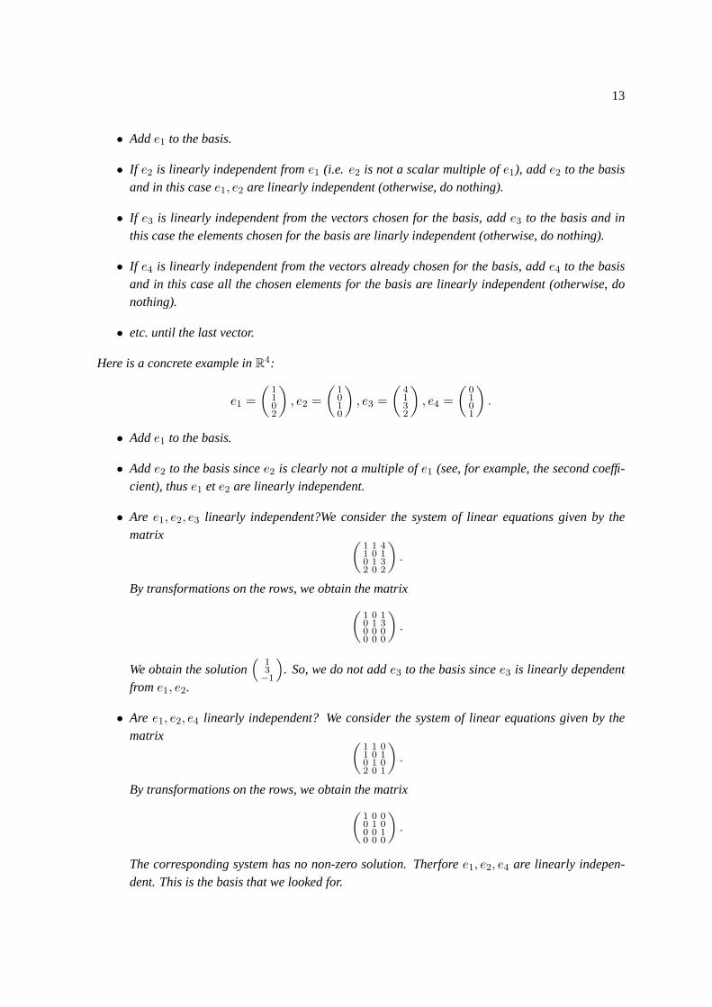
Example 1.25.How to compute a basis for a vector space generated by a finite set of vectors? (Sameanswer than almost always:) Solve a system of linear equations.Let V be aK-vector space generated by{e1, e2, . . . , em} (assumed all non-zero). We proceed asfollows:
13
• Adde1 to the basis.
• If e2 is linearly independent frome1 (i.e. e2 is not a scalar multiple ofe1), adde2 to the basisand in this casee1, e2 are linearly independent (otherwise, do nothing).
• If e3 is linearly independent from the vectors chosen for the basis, adde3 to the basis and inthis case the elements chosen for the basis are linarly independent (otherwise, do nothing).
• If e4 is linearly independent from the vectors already chosen for the basis, adde4 to the basisand in this case all the chosen elements for the basis are linearly independent (otherwise, donothing).
• etc. until the last vector.
Here is a concrete example inR4:
e1 =
(1102
), e2 =
(1010
), e3 =
(4132
), e4 =
(0101
).
• Adde1 to the basis.
• Adde2 to the basis sincee2 is clearly not a multiple ofe1 (see, for example, the second coeffi-cient), thuse1 ete2 are linearly independent.
• Are e1, e2, e3 linearly independent?We consider the system of linear equations given by thematrix (
1 1 41 0 10 1 32 0 2
).
By transformations on the rows, we obtain the matrix
(1 0 10 1 30 0 00 0 0
).
We obtain the solution(
13−1
). So, we do not adde3 to the basis sincee3 is linearly dependent
frome1, e2.
• Are e1, e2, e4 linearly independent? We consider the system of linear equations given by thematrix (
1 1 01 0 10 1 02 0 1
).
By transformations on the rows, we obtain the matrix
(1 0 00 1 00 0 10 0 0
).
The corresponding system has no non-zero solution. Therforee1, e2, e4 are linearly indepen-dent. This is the basis that we looked for.
14 1 RECALLS: VECTOR SPACES, BASES, DIMENSION, HOMOMORPHISMS
Dimension
Corollary 1.26. Let K be a field andV a K-vector space having a finiteK-basis. Then, all theK-bases ofV are finite and have the same cardinality.
This corollary allows us to make a very important definition, that of the dimensionof a vector space.The dimension measures the ’size’ or the ’number of degrees of freedom’of a vector space.
Definition 1.27. LetK be a field andV aK-vector space. IfV has a finiteK-basis of cardinalityn,we say thatV is ofdimensionn. If V has no finiteK-basis, we say thatV is of infinite dimension.Notation:dimK(V ).
Example 1.28. (a) The dimension of the standardK-vector spaceKn is equal ton.
(b) The zeroK-vector space({0},+, ·, 0) is of de dimension0 (and it is the only one).
(c) TheR-vector spaceF(N,R) is of infinite dimension.
Lemma 1.29. LetK be a field,V aK-vector space of dimensionn andW ≤ V a subspace.
(a) dimK(W ) ≤ dimK(V ).
(b) If dimK(W ) = dimK(V ), thenW = V .
The content of the following proposition is that anyK-linearly independent set can be completed tobecome aK-basis.
Proposition 1.30(Basisergänzungssatz). LetV be aK-vector space of dimensionn, E ⊆ V a finiteset such thatE generatesV and{e1, . . . , er} ⊂ V a subset that isK-linearly independent.Thenr ≤ n and there exister+1, er+2, . . . , en ∈ E such that{e1, . . . , en} is aK-basis ofV .
The proposition 1.30 can be shown in an abstract manner or in a constructive manner. Assume thatwe have elementse1, . . . , er that areK-linearly independent. Ifr = n, these elements are aK-basisby Lemma 1.29 (b) and we are done. Assume therefore thatr < n. We now run through the elementsof E until we find e ∈ E such thate1, . . . , er, e areK-linearly independent. Such an elemente
has to exist, otherwise the setE would be contained in the subspace generated bye1, . . . , er, ancould therefore not generateV . We call e =: er+1 and we have aK-linearly independent set ofcardinalityr + 1. It now suffices to continue this process until we arrive at aK-linearly independentset withn elements, which is automatically aK-basis.
Corollary 1.31. LetV be aK-vector space of finite dimensionn and letW ≤ V be a vector subspace.Then there exists a vector subspaceU ≤ V such thatV = U ⊕ V . Moreover, we have the equalitydim(V ) = dim(W ) + dim(U).We callU a complementofW in V . Note that this complement is not unique in general.
Proof. We choose aK-basisw1, . . . , wr of W and we use the proposition 1.30 to obtain vectorsu1, . . . , us ∈ V such thatw1, . . . , wr, u1, . . . , us form aK-basis ofV . PutU = 〈u1, . . . , us〉. Clearly,we haveV = U +W and alsoU ∩W = 0, soV = U ⊕W . The assertion concerning dimensionsfollows.
15
Proposition 1.32. Let V be aK-vector space of finite dimensionn. Let B ⊂ V be a subset ofcardinalityn. Then, the following assertions are equivalent.
(i) B is aK-basis.
(ii) B isK-linearly independent.
(iii) B generatesV .
Proof. For the equivalence between (i) and (ii) it suffices to observe that aK-linearly independentset of cardinalityn is necessarily maximal (thus aK-basis by Theorem 1.22), since if it was notmaximal, there would be a maximalK-linearly independent set of cardinality strictly larger thann,thus aK-basis of cardinality different fromn which is not possible by Corollary 1.26.Similarly, for the equivalence between (i) and (iii) it suffices to observe that a set of cardinalityn thatgeneratesV is necessarily minimal (thus aK-basis by Theorem 1.22), since if it was not minimal,there would be a minimal set of cardinality strictly smaller thann that generatesV , thus aK-basis ofcardinality different fromn.
Linear maps: homomorphisms of vector spaces
We start with the main idea :The (homo-)morphisms are maps that respect all the structures.
Definition 1.33. LetV,W beK-vector spaces. A map
ϕ : V →W
is calledK-linearor (homo-)morphism ofK-vector spacesif
∀ v1, v2 ∈ V : ϕ(v1 +V v2) = ϕ(v1) +W ϕ(v2)
and
∀ v ∈ V, ∀a ∈ K : ϕ(a ·V v) = a ·W ϕ(v).
A bijective homomorphism ofK-vector spaces is called anisomorphism. We often denote the iso-morphisms by a tilda:ϕ : V
∼−→ W . If there exists an isomorphismV → W , we often simply writeV ∼=W .
Example 1.34. (a) We start by the most important example. Letn ∈ N.
LetM =
a1,1 a1,2 · · · a1,na2,1 a2,2 · · · a2,n
......
. . ....
am,1 am,2 · · · am,n
be a matrix withn columns,m rows and with coefficients
in K (we denote the set of these matrices byMatm×n(K); this is also aK-vector space). Itdefines theK-linear map
ϕM : Kn → Km, v 7→Mv
16 1 RECALLS: VECTOR SPACES, BASES, DIMENSION, HOMOMORPHISMS
whereMv is the usual product for matrices. Explicitely,
ϕM (v) =Mv =
a1,1 a1,2 · · · a1,na2,1 a2,2 · · · a2,n
......
.. ....
am,1 am,2 · · · am,n
v1v2...vn
=
∑ni=1 a1,ivi∑ni=1 a2,ivi
...∑ni=1 am,ivi
.
TheK-linearity reads as
∀ a ∈ K ∀ v, w ∈ V :M ◦ (a · v + w) = a · (M ◦ v) +M ◦ w.
This equality is very easy to verify (you should have seen it in your Linear Algebra 1 course).
(b) Leta ∈ R. Then,ϕ : R → R, x 7→ ax isR-linear (this is the special casen = m = 1 of (a) if welook at the scalara as a matrix(a)). On the other hand, if0 6= b ∈ R, thenR → R, x 7→ ax+ b
is notR-linear!
(c) Letn ∈ N. Then, the mapϕ : F(N,R) → R, f 7→ f(n) isK-linear.
Definition 1.35. LetV,W beK-vector spaces andϕ : V → W aK-linear map. Thekernel ofϕ isdefined as
ker(ϕ) = {v ∈ V | ϕ(v) = 0}.
Proposition 1.36. LetV,W beK-vector spaces andϕ : V →W aK-linear map.
(a) Im(ϕ) is a vector subspace ofW .
(b) ker(ϕ) is a vector subspace ofV .
(c) ϕ is surjective if and only ifIm(ϕ) =W .
(d) ϕ is injective if and only ifker(ϕ) = 0.
(e) Ifϕ is an isomorphism, its inverse is one too (in particular, its inverse is alsoK-linear).
Definition 1.37. LetM ∈ Matm×n(K) be a matrix. We callrank of columnsofM the dimension ofthe vector subspace ofKm generates by the columns ofM . We use the notationrk(M).
Similarly, we define therank of rowsofM the dimension of the vector subspace ofKn generated bythe rows ofM . More formally, it is the rank ofM tr, the transpose matrix.
We will see towards the end of the course that for any matrix, the rank of columns is equal to the rankof rows. This explains why we did not mention the word “ columns” in the notationof the rank.
If ϕM : Kn → Km is theK-linear map associated toM , then
rk(M) = dim(Im(ϕM ))
since the image ofϕM is precisely the vector space generated by the columns ofM .
17
Corollary 1.38. (a) Letϕ : V → X be aK-linear map between twoK-vector spaces. We assumethatV has finite dimension. Then,
dim(V ) = dim(ker(ϕ)) + dim(Im(ϕ)).
(b) LetM ∈ Matm×n(K) be a matrix. Then, we have
n = dim(ker(M)) + rk(M).
Proof. (a) LetW = ker(ϕ). We choose a complementU ≤ V such thatV = U ⊕W by Corol-lary 1.31. AsU ∩W = 0, the mapϕ|U : U → X is injective. Moreover,ϕ(V ) = ϕ(U+W ) = ϕ(U)
shows thatIm(ϕ) is equal toϕ(U). Consequently,dim(Im(ϕ)) = dim(ϕ(U)) = dim(U), thus thedesired equality.(b) follows directly from (a) by the above considerations.
Part (b) is very useful for computing the kernel of a matrix: if we know therank ofM , we deduce thedimension of the kernel by the formula
dim(ker(M)) = n− rk(M).
Gauß’ algorithm in terms of matrices
We consider three types of matrices:
Definition 1.39. For 0 6= λ ∈ K and 1 ≤ i, j ≤ n, i 6= j, we define the following matrices inMatn×n(K), calledelementary matrices:
• Pi,j is equal to the identityidn except that thei-th and thej-th rows are exchanged (or, equiv-
alently, thei-th and thej-th column are exchanged):Pi,j =
1...
10 111
1 01
...1
.
• Si(λ) is equal to the identityidn except that the coefficient(i, i) on the diagonal isλ (instead
of 1): Si(λ) =
1...
1λ
1...
1
.
• Qi,j(λ) is equal to the identityidn except that the coefficient(i, j) isλ (instead of0): Qi,j(λ) =
1...
... λ...
1
.
18 1 RECALLS: VECTOR SPACES, BASES, DIMENSION, HOMOMORPHISMS
The elementary matrices have a signification for the operations of matrices.
Lemma 1.40. Letλ ∈ K, i, j, n,m ∈ N>0, i 6= j andM ∈ Matn×m(K).
(a) Pi,jM is the matrix obtained fromM by exchanging thei-th and thej-th row.MPi,j is the matrix obtained fromM by exchanging thei-th and thej-th coulumn.
(b) Si(λ)M is the matrix obtained fromM by multiplying thei-th row byλ.MSi(λ) is the matrix obtained fromM by multiplying thei-th column byλ.
(c) Qi,j(λ)M is the matrix obtained fromM by addingλ times thej-th row to thei-th row.MQi,j(λ) is the matrix obtained fromM by addingλ times thei-th column to thej-th column.
Proof. Easy computations.
Proposition 1.41. Let M ∈ Matn×m(K) be a matrix and letN ∈ Matn×m(K) be the matrixobtained fromM by making operations on the rows (as in Gauß’ algorithm).
(a) Then there exist matricesC1, . . . , Cr (for somer ∈ N) chosen among the matrices of Defini-tion 1.39 such that(C1 · · ·Cr) ·M = N .
(b) ker(M) = ker(N) and thus Gauß’ row reduction algorithm can be used in order to compute thekernel of a matrix.
Proof. (a) By Lemma 1.40 any operation on the rows can be done by left multiplication byone of thematrices of Definition 1.39.
(b) All the matrices of Definition 1.39 are invertible, thus do not change the kernel.
Similarly to (b), any operation on the columns corresponds to right multiplication by one of the ma-trices of Definition 1.39. Thus, ifN is a matrix obtained from a matrixM by doing operations onthe columns, there exist matricesC1, . . . , Cr (for somer ∈ N) chosen among the matrices of Defini-tion 1.39 such thatM · (C1 · · ·Cr) = N . Since the matricesCi are invertible, we also have
im(M) = im(N),
and in particular the rank ofM is equal to the rank ofN .
Often we are interested in knowing a matrixC such thatCM = N whereN is obtained fromM byoperations on the rows.
In order to obtain this, it suffices to observe thatC · id = C, hence applyingC is equivalent to doingoperations on the corresponding rows of the matrixid. In the following example, we see how this isdone in practice.
Example 1.42.LetM =
1 2 3
4 5 6
7 8 9
. We write the augmented matrix and do the operations on the
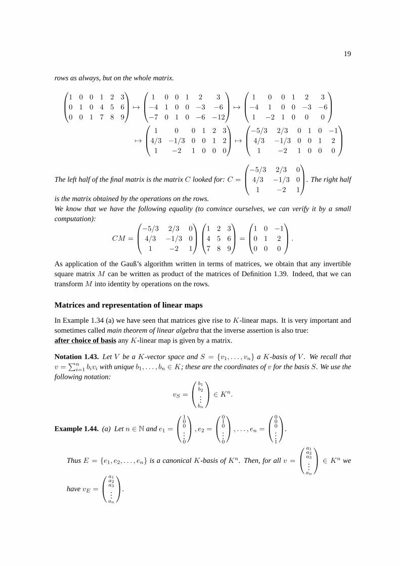
19
rows as always, but on the whole matrix.
1 0 0 1 2 3
0 1 0 4 5 6
0 0 1 7 8 9
7→
1 0 0 1 2 3
−4 1 0 0 −3 −6
−7 0 1 0 −6 −12
7→
1 0 0 1 2 3
−4 1 0 0 −3 −6
1 −2 1 0 0 0
7→
1 0 0 1 2 3
4/3 −1/3 0 0 1 2
1 −2 1 0 0 0
7→
−5/3 2/3 0 1 0 −1
4/3 −1/3 0 0 1 2
1 −2 1 0 0 0
The left half of the final matrix is the matrixC looked for:C =
−5/3 2/3 0
4/3 −1/3 0
1 −2 1
. The right half
is the matrix obtained by the operations on the rows.We know that we have the following equality (to convince ourselves, we can verify it by a smallcomputation):
CM =
−5/3 2/3 0
4/3 −1/3 0
1 −2 1
1 2 3
4 5 6
7 8 9
=
1 0 −1
0 1 2
0 0 0
.
As application of the Gauß’s algorithm written in terms of matrices, we obtain that any invertiblesquare matrixM can be written as product of the matrices of Definition 1.39. Indeed, that wecantransformM into identity by operations on the rows.
Matrices and representation of linear maps
In Example 1.34 (a) we have seen that matrices give rise toK-linear maps. It is very important andsometimes calledmain theorem of linear algebrathat the inverse assertion is also true:after choice of basisanyK-linear map is given by a matrix.
Notation 1.43. Let V be aK-vector space andS = {v1, . . . , vn} a K-basis ofV . We recall thatv =
∑ni=1 bivi with uniqueb1, . . . , bn ∈ K; these are the coordinates ofv for the basisS. We use the
following notation:
vS =
b1b2...bn
∈ Kn.
Example 1.44. (a) Letn ∈ N ande1 =
100...0
, e2 =
010...0
, . . . , en =
000...1
.
ThusE = {e1, e2, . . . , en} is a canonicalK-basis ofKn. Then, for allv =
a1a2a3...an
∈ Kn we
havevE =
a1a2a3...an
.
20 1 RECALLS: VECTOR SPACES, BASES, DIMENSION, HOMOMORPHISMS
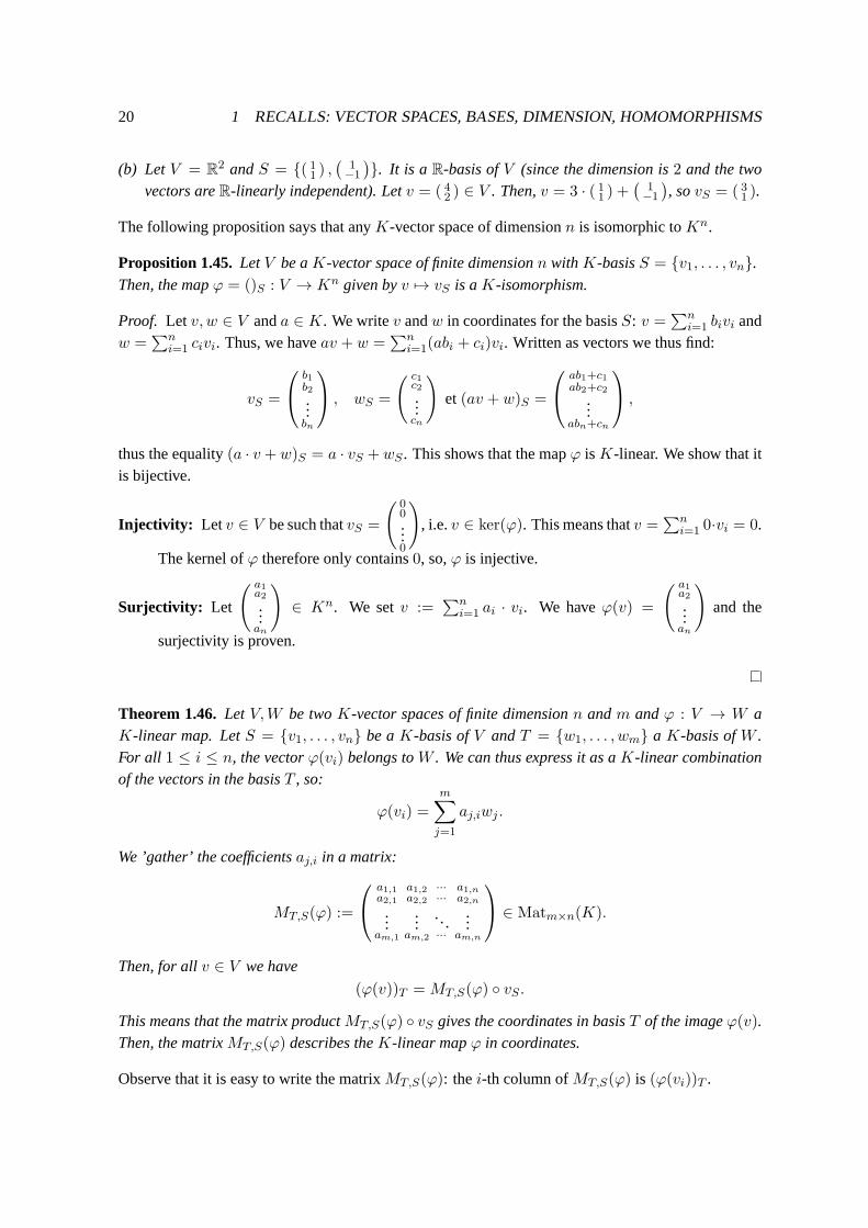
(b) LetV = R2 andS = {( 11 ) ,(
1−1
)}. It is a R-basis ofV (since the dimension is2 and the two
vectors areR-linearly independent). Letv = ( 42 ) ∈ V . Then,v = 3 · ( 11 ) +(
1−1
), sovS = ( 31 ).
The following proposition says that anyK-vector space of dimensionn is isomorphic toKn.
Proposition 1.45. LetV be aK-vector space of finite dimensionn withK-basisS = {v1, . . . , vn}.
Then, the mapϕ = ()S : V → Kn given byv 7→ vS is aK-isomorphism.
Proof. Let v, w ∈ V anda ∈ K. We writev andw in coordinates for the basisS: v =∑n
i=1 bivi andw =
∑ni=1 civi. Thus, we haveav + w =
∑ni=1(abi + ci)vi. Written as vectors we thus find:
vS =
b1b2...bn
, wS =
( c1c2...cn
)et (av + w)S =
ab1+c1ab2+c2
...abn+cn
,
thus the equality(a · v +w)S = a · vS +wS . This shows that the mapϕ isK-linear. We show that itis bijective.
Injectivity: Letv ∈ V be such thatvS =
( 00...0
), i.e.v ∈ ker(ϕ). This means thatv =
∑ni=1 0·vi = 0.
The kernel ofϕ therefore only contains0, so,ϕ is injective.
Surjectivity: Let
( a1a2...an
)∈ Kn. We setv :=
∑ni=1 ai · vi. We haveϕ(v) =
( a1a2...an
)and the
surjectivity is proven.
Theorem 1.46. Let V,W be twoK-vector spaces of finite dimensionn andm andϕ : V → W aK-linear map. LetS = {v1, . . . , vn} be aK-basis ofV andT = {w1, . . . , wm} a K-basis ofW .For all 1 ≤ i ≤ n, the vectorϕ(vi) belongs toW . We can thus express it as aK-linear combinationof the vectors in the basisT , so:
ϕ(vi) =m∑
j=1
aj,iwj .
We ’gather’ the coefficientsaj,i in a matrix:
MT,S(ϕ) :=
a1,1 a1,2 ··· a1,na2,1 a2,2 ··· a2,n...
......
...am,1 am,2 ··· am,n
∈ Matm×n(K).
Then, for allv ∈ V we have
(ϕ(v))T =MT,S(ϕ) ◦ vS .
This means that the matrix productMT,S(ϕ) ◦ vS gives the coordinates in basisT of the imageϕ(v).Then, the matrixMT,S(ϕ) describes theK-linear mapϕ in coordinates.
Observe that it is easy to write the matrixMT,S(ϕ): thei-th column ofMT,S(ϕ) is (ϕ(vi))T .
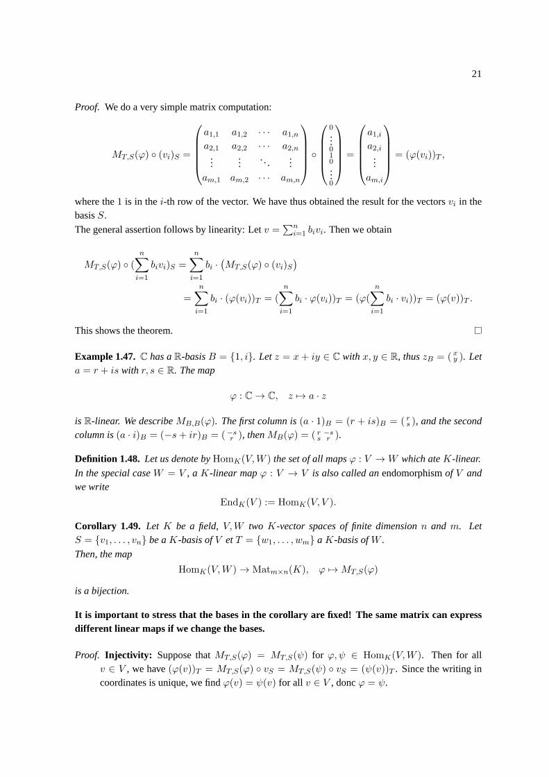
21
Proof. We do a very simple matrix computation:
MT,S(ϕ) ◦ (vi)S =
a1,1 a1,2 · · · a1,na2,1 a2,2 · · · a2,n
......
. . ....
am,1 am,2 · · · am,n
◦
0...010...0
=
a1,ia2,i
...am,i
= (ϕ(vi))T ,
where the1 is in thei-th row of the vector. We have thus obtained the result for the vectorsvi in thebasisS.
The general assertion follows by linearity: Letv =∑n
i=1 bivi. Then we obtain
MT,S(ϕ) ◦ (n∑
i=1
bivi)S =n∑
i=1
bi ·(MT,S(ϕ) ◦ (vi)S
)
=n∑
i=1
bi · (ϕ(vi))T = (n∑
i=1
bi · ϕ(vi))T = (ϕ(n∑
i=1
bi · vi))T = (ϕ(v))T .
This shows the theorem.
Example 1.47.C has aR-basisB = {1, i}. Letz = x+ iy ∈ C with x, y ∈ R, thuszB = ( xy ). Leta = r + is with r, s ∈ R. The map
ϕ : C → C, z 7→ a · z
is R-linear. We describeMB,B(ϕ). The first column is(a · 1)B = (r + is)B = ( rs ), and the secondcolumn is(a · i)B = (−s+ ir)B = (−sr ), thenMB(ϕ) = ( r −s
s r ).
Definition 1.48. Let us denote byHomK(V,W ) the set of all mapsϕ : V →W which ateK-linear.
In the special caseW = V , aK-linear mapϕ : V → V is also called anendomorphismof V andwe write
EndK(V ) := HomK(V, V ).
Corollary 1.49. Let K be a field,V,W two K-vector spaces of finite dimensionn andm. LetS = {v1, . . . , vn} be aK-basis ofV etT = {w1, . . . , wm} aK-basis ofW .
Then, the map
HomK(V,W ) → Matm×n(K), ϕ 7→MT,S(ϕ)
is a bijection.
It is important to stress that the bases in the corollary are fixed! The same matrix can expressdifferent linear maps if we change the bases.
Proof. Injectivity: Suppose thatMT,S(ϕ) = MT,S(ψ) for ϕ, ψ ∈ HomK(V,W ). Then for allv ∈ V , we have(ϕ(v))T = MT,S(ϕ) ◦ vS = MT,S(ψ) ◦ vS = (ψ(v))T . Since the writing incoordinates is unique, we findϕ(v) = ψ(v) for all v ∈ V , doncϕ = ψ.
22 1 RECALLS: VECTOR SPACES, BASES, DIMENSION, HOMOMORPHISMS
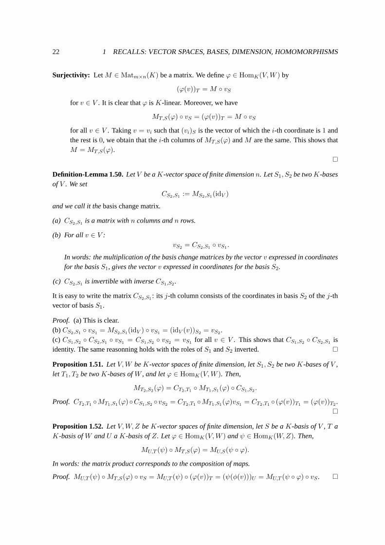
Surjectivity: LetM ∈ Matm×n(K) be a matrix. We defineϕ ∈ HomK(V,W ) by
(ϕ(v))T =M ◦ vSfor v ∈ V . It is clear thatϕ isK-linear. Moreover, we have
MT,S(ϕ) ◦ vS = (ϕ(v))T =M ◦ vSfor all v ∈ V . Takingv = vi such that(vi)S is the vector of which thei-th coordinate is1 andthe rest is0, we obtain that thei-th columns ofMT,S(ϕ) andM are the same. This shows thatM =MT,S(ϕ).
Definition-Lemma 1.50. LetV be aK-vector space of finite dimensionn. LetS1, S2 be twoK-basesof V . We set
CS2,S1 :=MS2,S1(idV )
and we call it thebasis change matrix.
(a) CS2,S1 is a matrix withn columns andn rows.
(b) For all v ∈ V :vS2 = CS2,S1 ◦ vS1 .
In words: the multiplication of the basis change matrices by the vectorv expressed in coordinatesfor the basisS1, gives the vectorv expressed in coordinates for the basisS2.
(c) CS2,S1 is invertible with inverseCS1,S2 .
It is easy to write the matrixCS2,S1 : its j-th column consists of the coordinates in basisS2 of thej-thvector of basisS1.
Proof. (a) This is clear.(b)CS2,S1 ◦ vS1 =MS2,S1(idV ) ◦ vS1 = (idV (v))S2 = vS2 .(c) CS1,S2 ◦ CS2,S1 ◦ vS1 = CS1,S2 ◦ vS2 = vS1 for all v ∈ V . This shows thatCS1,S2 ◦ CS2,S1 isidentity. The same reasonning holds with the roles ofS1 andS2 inverted.
Proposition 1.51. LetV,W beK-vector spaces of finite dimension, letS1, S2 be twoK-bases ofV ,let T1, T2 be twoK-bases ofW , and letϕ ∈ HomK(V,W ). Then,
MT2,S2(ϕ) = CT2,T1 ◦MT1,S1(ϕ) ◦ CS1,S2 .
Proof. CT2,T1 ◦MT1,S1(ϕ)◦CS1,S2 ◦vS2 = CT2,T1 ◦MT1,S1(ϕ)vS1 = CT2,T1 ◦ (ϕ(v))T1 = (ϕ(v))T2 .
Proposition 1.52. LetV,W,Z beK-vector spaces of finite dimension, letS be aK-basis ofV , T aK-basis ofW andU aK-basis ofZ. Letϕ ∈ HomK(V,W ) andψ ∈ HomK(W,Z). Then,
MU,T (ψ) ◦MT,S(ϕ) =MU,S(ψ ◦ ϕ).
In words: the matrix product corresponds to the composition of maps.
Proof. MU,T (ψ) ◦MT,S(ϕ) ◦ vS =MU,T (ψ) ◦ (ϕ(v))T = (ψ(φ(v)))U =MU,T (ψ ◦ ϕ) ◦ vS .
23
Appendix: existence of bases
For lack of time, this section will neither be taught, neither be examined.In the lecture course “Structures mathématiques” we have introduced the sets from an intuitive andnon-rigurous point of view. A strict treatment can only take place in a logic course at a more advancedstage (such a course is not offered at the UL for the moment – you can consult books for more details).In set theory, there is an important axiom: the ’axiom of choix’.1 In set theory one shows ’Zorn’sLemma’ which says that the axiom of choice is equivalent to the following assertion.
Axiom 1.53 (Zorn’s Lemma). Let S be a non-empty set and≤ a partial order onS.2 We make thefollowing hypothesis: Any subsetT ⊆ S which is totally ordered3 has an upper bound.4
Then,S has a maximal element.5
To show how to apply Zorn’s Lemma, we prove that ant vector space has abasis. If you have seenthis assertion in your Linear Algebra 1 lecture course, then it was for finite-dimensional vector spacesbecause the general case is in fact equivalent to the axiom of choice (an thus to Zorn’s Lemma).
Proposition 1.54. LetK be a field andV 6= {0} aK-vector space. Then,V has aK-basis.
Proof. We recall some notions of linear algebra. A finite subsetG ⊆ V is calledK-linearly indepen-dentif the only linear combination0 =
∑g∈G agg with ag ∈ K is that whereag = 0 for all g ∈ G.
More generally, a non-necessarily finite subsetG ⊆ V is calledK-linearly independentif any finitesubsetH ⊆ G is K-linearly independent. A subsetG ⊆ V is called aK-basisif it is K-linearlyindependet and generatesV .6
We want to use Zorn’s Lemma 1.53. Let
S := {G ⊆ V subset| G isK-linearly independent}.
The setS is non-empty sinceG = {v} isK-linearly independent for all0 6= v ∈ V . The inclusion ofsets ’⊆’ defines an order relation onS (it is obvious – see Algebra 1).We verify that the hypothesis of Zorn’s Lemma is satisfied: LetT ⊆ S be a totally ordered subset. Wehave to produce an upper boundE ∈ S for T . We setE :=
⋃G∈T G. It is clear thatG ⊆ E for all
G ∈ T . One has to show thatE ∈ S, thus thatE isK-linearly independent. LetH ⊆ E be a subsetof cardinalityn. We show by induction onn that there existsG ∈ T such thatH ⊆ G. The assertionis clear forn = 1. Assume it proven forn − 1 and writeH = H ′ ⊔ {h}. The existG′, G ∈ T such
1Axiom of choice: LetX be a set of which the elements are non-empty sets. Then there exists a function f definedonX which to anyM ∈ X associates an element ofM . Such a function is called “function of choice”.
2e recall that by definition the three following points are satisfied:
• s ≤ s for all s ∈ S.
• If s ≤ t andt ≤ s for s, t ∈ S, thens = t.
• If s ≤ t andt ≤ u for s, t, u ∈ S, thens ≤ u.
3T is totally ordered ifT is ordered and for all pairs, t ∈ T we haves ≤ t or t ≤ s.4g ∈ S is an upper bound forT if t ≤ g for all t ∈ T .5m ∈ S is maximal if for alls ∈ S such thatm ≤ s we havem = s.6i.e.: any elementv ∈ V writes asv =
∑n
i=1 aigi with n ∈ N, a1, . . . , an ∈ K etg1, . . . , gn ∈ G.
24 2 RECALLS: DETERMINANTS
thatH ′ ⊆ G′ (by induction hypothesis because the cardinality ofH ′ is n− 1) andh ∈ G (by the casen = 1). By the fact thatT is totally ordered, we haveG ⊆ G′ or G′ ⊆ G. In both cases we obtainthatH is a subset ofG or ofG′. SinceH is a finite subset of a set which isK-linearly independent,H is too. Thus,E isK-linearly independent.Zorn’s Lemma gives us a maximal elementB ∈ S. We show thatB is aK-basis ofV . As elementof S, B is K-linearly independent. One has to show thatB generatesV . Suppose that this is notthe case and let us takev ∈ V which cannot be written as aK-linear combination of the elementsin B. Then the setG := B ∪ {v} is alsoK-linearly independent, since anyK-linear combination0 = av+
∑ni=1 aibi with n ∈ N, a, a1, . . . , an ∈ K andb1, . . . , bn ∈ B with a 6= 0 would lead to the
contradictionv =∑n
i=1−aia bi (note thata = 0 corresponds to aK-linear combination inB which is
K-linearly independent). But,B ( G ∈ S contradicts maximality ofB.
2 Recalls: Determinants
Goals:
• Master the definition and the fundamental properties of the determinants;
• be able to compute determinants;
• know examples and be able to prove simple properties.
Définition et premières propriétés
The determinants have been introduced the previous semester. Here we recall them form anotherviewpoint: we start from the computation rules. Actually, our first proposition can be used as adefinition; it is Weierstraß’ axiomatic (see the book of Fischer).In this section we allow thatK is a commutative ring (but you can still takeK = R orK = C withoutloss of information).
If M =
m1,1 m1,2 ··· m1,nm2,1 m2,2 ··· m2,n
......
......
mn,1 mn,2 ··· mn,n
is a matrix, we denote bymi = (mi,1 mi,2 ··· mi,n ) its i-th row, i.e.
M =
( m1m2
...mn
).
Proposition 2.1. Letn ∈ N>0. Thedeterminantis a map
det : Matn×n(K) → K, M 7→ det(M)
such that
D1 det is K-linear in each row, that is, for all1 ≤ i ≤ n, if mi = r + λs with λ ∈ K, r =
( r1 r2 ··· rn ) ands = ( s1 s2 ··· sn ), then
det
m1
...mi−1mimi+1
...mn
= det
m1
...mi−1
r+λsmi+1
...mn
= det
m1
...mi−1r
mi+1
...mn
+ λ · det
m1
...mi−1s
mi+1
...mn
.
25
D2 det is alternating, that is, if two of the rows ofM are equal, thendet(M) = 0.
D3 det is normalized, that is,det(idn) = 1 whereidn is the identity.
Proof. This has been proven in the course of linear algebra in the previous semester.
We often use the notation∣∣∣∣∣∣
m1,1 m1,2 ··· m1,nm2,1 m2,2 ··· m2,n
......
......
mn,1 mn,2 ··· mn,n
∣∣∣∣∣∣:= det
m1,1 m1,2 ··· m1,nm2,1 m2,2 ··· m2,n
......
......
mn,1 mn,2 ··· mn,n
.
Proposition 2.2. The following properties are satisfied.
D4 For all λ ∈ K, we havedet(λ ·M) = λn det(M).
D5 If a row is equal to0, thendet(M) = 0.
D6 If M is obtained fromM by swapping two rows, thendet(M) = − det(M).
D7 Letλ ∈ A andi 6= j. If M is obtained fromM by addingλ times thej-th row to thei-th row,thendet(M) = det(M).
Proof. D4 This follows from the linearity (D1).D5 This follows from the linearity (D1).
D6 Let us say that thei-th and thej-the row are swapped. ThusM =
m1
...mi
...mj
...mn
andM =
m1
...mj
...mi
...mn
.
det(M) + det(M) = det
m1
...mi
...mj
...mn
+ det
m1
...mj
...mi
...mn
D2= det
m1
...mj
...mj
...mn
+ det
m1
...mi
...mj
...mn
+ det
m1
...mj
...mi
...mn
+ det
m1
...mi
...mi
...mn
D1= det
m1
...mi+mj
...mj
...mn
+ det
m1
...mi+mj
...mi
...mn
= det
m1
...mi+mj
...mi+mj
...mn
D2= 0.
26 2 RECALLS: DETERMINANTS
D7 We have
det(M) = det
m1
...mi+λmj
...mj
...mn
D1= det
m1
...mi
...mj
...mn
+ λ · det
m1
...mj
...mj
...mn
D2= det(M) + λ · 0 = det(M).
Proposition 2.3. The following properties are satisfied.
D8 If M is of (upper) triangular form
λ1 m1,2 m1,3 ··· m1,n
0 λ2 m2,3 ··· m2,n
0 0 λ3 ··· m3,n
......
... ......
0 0 0 ··· λn
,
thendet(M) =∏ni=1 λi.
D9 If M is a bloc matrix(A B0 C
)with square matricesA andC, thendet(M) = det(A) · det(C).
Proof. Left to the reader.
Leibniz’ Formula
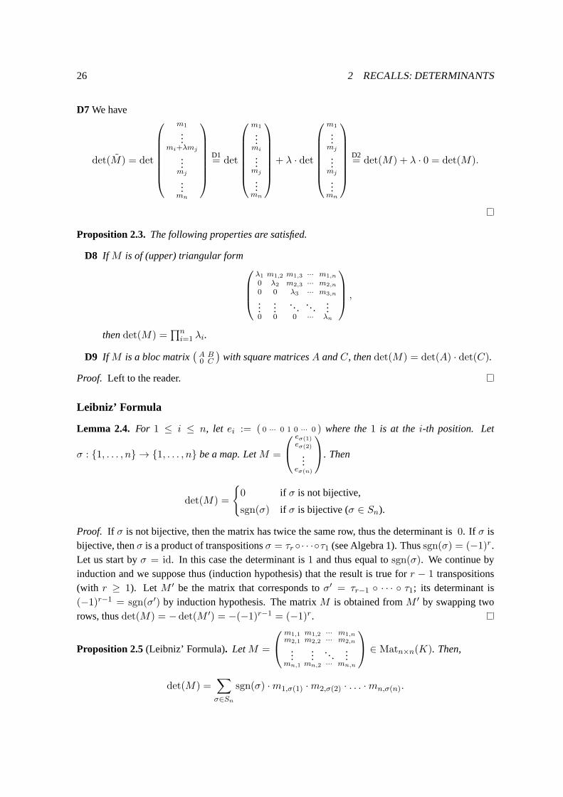
Lemma 2.4. For 1 ≤ i ≤ n, let ei := ( 0 ··· 0 1 0 ··· 0 ) where the1 is at thei-th position. Let
σ : {1, . . . , n} → {1, . . . , n} be a map. LetM =
eσ(1)eσ(2)
...eσ(n)
. Then
det(M) =
{0 if σ is not bijective,
sgn(σ) if σ is bijective (σ ∈ Sn).
Proof. If σ is not bijective, then the matrix has twice the same row, thus the determinant is0. If σ isbijective, thenσ is a product of transpositionsσ = τr ◦· · ·◦τ1 (see Algebra 1). Thussgn(σ) = (−1)r.Let us start byσ = id. In this case the determinant is1 and thus equal tosgn(σ). We continue byinduction and we suppose thus (induction hypothesis) that the result is truefor r − 1 transpositions(with r ≥ 1). Let M ′ be the matrix that corresponds toσ′ = τr−1 ◦ · · · ◦ τ1; its determinant is(−1)r−1 = sgn(σ′) by induction hypothesis. The matrixM is obtained fromM ′ by swapping tworows, thusdet(M) = − det(M ′) = −(−1)r−1 = (−1)r.
Proposition 2.5(Leibniz’ Formula). LetM =
m1,1 m1,2 ··· m1,nm2,1 m2,2 ··· m2,n
......
......
mn,1 mn,2 ··· mn,n
∈ Matn×n(K). Then,
det(M) =∑
σ∈Sn
sgn(σ) ·m1,σ(1) ·m2,σ(2) · . . . ·mn,σ(n).
27
Proof. The linearity of rows (D1) gives us
det(M) =n∑
i1=1
m1,i1
∣∣∣∣∣∣
ei1m2m3
...mn
∣∣∣∣∣∣=
n∑
i1=1
n∑
i2=1
m1,i1m2,i2
∣∣∣∣∣∣∣
ei1ei2m3
...mn
∣∣∣∣∣∣∣
= · · · =n∑
i1=1
n∑
i2=1
· · ·n∑
in=1
m1,i1m2,i2 · · ·mn,in
∣∣∣∣∣∣∣
ei1ei2ei3...ein
∣∣∣∣∣∣∣
=∑
σ∈Sn
m1,σ(1)m2,σ(2) · · ·mn,σ(n) · sgn(σ),
where the last equality results from Lemma 2.4. Note that the determinant of the matrix
ei1ei2ei3...ein
is
non-zero only if theij ’s are all different; this allows us to identify it with the permutationσ(j) = ij .That the determinant is unique is clear because it is a function of the coefficients of the matrix.
Corollary 2.6. LetM ∈ Matn×n(K). We denote byM tr the transposed matrix. Then,det(M) =
det(M tr).
Proof. We use Leibniz’ Formula 2.5. Note first thatsgn(σ) = sgn(σ−1) for all σ in Sn sincesgn is ahomomorphism of groups,1−1 = 1 et (−1)−1 = −1. Write now
m1,σ(1)m2,σ(2) · · ·mn,σ(n) = mσ−1(σ(1)),σ(1)mσ−1(σ(2)),σ(2) · · ·mσ−1(σ(n)),σ(n)
= mσ−1(1),1mσ−1(2),2 · · ·mσ−1(n),n,
where for the last equality we have only written the product in another order since the elementsσ(1), σ(2), . . . , σ(n) run through1, 2, . . . , n (only in another order).We thus have
det(M) =∑
σ∈Sn
sgn(σ)m1,σ(1)m2,σ(2) · · ·mn,σ(n)
=∑
σ∈Sn
sgn(σ−1)mσ−1(1),1mσ−1(2),2 · · ·mσ−1(n),n
=∑
σ∈Sn
sgn(σ−1)mtr1,σ−1(1)m
tr2,σ−1(2) · · ·mtr
n,σ−1(n)
=∑
σ∈Sn
sgn(σ)mtr1,σ(1)m
tr2,σ(2) · · ·mtr
n,σ(n)
= det(M tr),
where we have used the bijectionSn → Sn given byσ 7→ σ−1; it is thus makes no change if the sumruns throughσ ∈ Sn or through the inverses.
Corollary 2.7. The rulesD1 to D9 are also true for the columns instead of the rows.
Proof. By taking the transpose of a matrix, the rows become columns, but by Corollary 2.6, thedeterminant does not change.

28 2 RECALLS: DETERMINANTS
Laplace expansion
Definition 2.8. Letn ∈ N>0 andM =
m1,1 m1,2 ··· m1,nm2,1 m2,2 ··· m2,n
......
......
mn,1 mn,2 ··· mn,n
∈ Matn×n(K). For 1 ≤ i, j ≤ n we
define the matrices
Mi,j =
m1,1 ··· m1,j−1 0 m1,j+1 ··· m1,n
......
......
......
...mi−1,1 ··· mi−1,j−1 0 mi−1,j+1 ··· mi−1,n
0 ··· 0 1 0 ··· 0mi+1,1 ··· mi+1,j−1 0 mi+1,j+1 ··· mi+1,n
......
......
......
...mn,1 ··· mn,j−1 0 mn,j+1 ··· mn,n
∈ Matn×n(A)
and
M ′i,j =
m1,1 ··· m1,j−1 m1,j+1 ··· m1,n
......
......
......
mi−1,1 ··· mi−1,j−1 mi−1,j+1 ··· mi−1,nmi+1,1 ··· mi+1,j−1 mi+1,j+1 ··· mi+1,n
......
......
......
mn,1 ··· mn,j−1 mn,j+1 ··· mn,n
∈ Matn−1×n−1(A).
Moreover, letMi,j be the matrix obtained fromM by replacing thej-th column by
0...010...0
, where the
1 is at thei-th position.The determinantsdet(M ′
i,j) are called theminorsofM .
Lemma 2.9. Letn ∈ N>0 andM ∈ Matn×n(K). For all 1 ≤ i, j ≤ n, we have
(a) det(Mi,j) = (−1)i+j · det(M ′i,j),
(b) det(Mi,j) = det(Mi,j).
Proof. (a) By swappingi rows, the row with the zeros is the first one. By swappingj columns, weobtain the matrix
1 0 ··· 0 0 ··· 00 m1,1 ··· m1,j−1 m1,j+1 ··· m1,n
......
......
......
...0 mi−1,1 ··· mi−1,j−1 mi−1,j+1 ··· mi−1,n
0 mi+1,1 ··· mi+1,j−1 mi+1,j+1 ··· mi+1,n
......
......
......
...0 mn,1 ··· mn,j−1 mn,j+1 ··· mn,n
∈ Matn×n(A)
of which the determinant isdet(M ′i,j) (because ofD9), which proves the result.
(b) Adding−mi,k times thej-th column to thek-th column ofMi,j makes the coefficient(i, k) equalto 0 for k 6= i without changing the determinant (Corollary 2.7).
Proposition 2.10(Laplace expansion for the rows). Let n ∈ N>0. For all 1 ≤ i ≤ n, we have theequality
det(M) =n∑
j=1
(−1)i+jmi,j det(M′i,j)
29
Proof. By the axiomD2 (linearity in the rows), we have
det(M) =
n∑
j=1
mi,j
∣∣∣∣∣∣∣∣∣∣
m1
...mi−1ei
mi+1
...mn
∣∣∣∣∣∣∣∣∣∣
=
n∑
j=1
mi,j det(Mi,j) =
n∑
j=1
(−1)i+jmi,j det(M′i,j).
Corollary 2.11 (Laplace expansion for the columns). For all n ∈ N>0 and all 1 ≤ j ≤ n, we havethe formula
det(M) :=n∑
i=1
(−1)i+jmi,j det(M′i,j).
Proof. It suffices to apply Proposition 2.10 to the transposed matrix and to remember (Corollary 2.6)that the determinant of the transposed matrix is the same.
Note that the formulas of Laplace can be written as
det(M) =
n∑
j=1
mi,j det(Mi,j) =
n∑
i=1
mi,j det(Mi,j).
Adjoint matrices
Definition 2.12. Theadjoint matrixadj(M) = M# = (m#i,j) of the matrixM ∈ Matn×n(A) is
defined bym#i,j := det(Mj,i) = (−1)i+j det(M ′
j,i).
Proposition 2.13. For all matrixM ∈ Matn×n(K), we have the equality
M# ·M =M ·M# = det(M) · idn.
Proof. LetN = (ni,j) :=M ·M#. We computeni,j :
ni,j =
n∑
k=1
m#i,kmk,j =
n∑
k=1
det(Mk,i)mk,j .
If i = j, we findni,i = det(M) by Laplace’s formula. But we don’t need to use this formula and wecontinue in generality by usingdet(Mk,i) = det(Mk,i) by Lemma 2.9 (b). The linearity in thei-thcolumn shows that
∑nk=1 det(Mk,i)mk,j is the determinant of the matrix of which thei-th column is
replaced by thej-th column. Ifi = j, this matrix isM , somi,i = det(M). If i 6= j, this determinant(and thusni,j) is 0 because two of the columns are equal.The proof forM# ·M is similar.
Corollary 2.14. LetM ∈ Matn×n(K).
(a) If det(M) is invertible inK (for K a field this meansdet(M) 6= 0), thenM is invertible and theinverse matrixM−1 is equal to 1
det(M)M#.
30 3 EIGENVALUES
(b) If M is invertible, thenM−1 det(M) =M#.
Proof. Proposition 2.13.
We finish this recall by the following fundamental result.
Proposition 2.15. LetM,N ∈ Matn×n(K).
(a) det(M ·N) = det(M) · det(N).
(b) The following statements are equivalent:
(i) M is invertible;
(ii) det(M) is invertible.
In this case:det(M−1) = 1det(M) .
Proof. (a) was proved in the lecture Linear Algebra 1.(b) is obvious because of Proposition 2.13.
3 Eigenvalues
Goals:
• Master the definition and fundamental properties of eigenvalues and eigenvectors;
• be able to compute eigenspaces;
• know examples and be able to prove simple properties.
Example 3.1. (a) ConsiderM = ( 3 00 2 ) ∈ Mat2×2(R). We have:
• ( 3 00 2 ) (
10 ) = 3 · ( 10 ) and
• ( 3 00 2 ) (
01 ) = 2 · ( 01 ).
(b) ConsiderM = ( 3 10 2 ) ∈ Mat2×2(R). We have:
• ( 3 10 2 ) (
a0 ) = 3 · ( a0 ) for all a ∈ R.
• ( 3 10 2 ) (
ab ) =
(3a+b2b
)= 2 · ( ab ) ⇔ a = −b. Thus for alla ∈ R, we have
( 3 10 2 ) (
a−a ) = 2 · ( a
−a ).
(c) ConsiderM =(
5 1−4 10
)∈ Mat2×2(R). We have:
•(
5 1−4 10
)( 14 ) = 9 ( 14 ) and
•(
5 1−4 10
)( 11 ) = 6 ( 11 ).
(d) ConsiderM = ( 2 10 2 ) ∈ Mat2×2(R). We have:
• ( 2 10 2 ) (
a0 ) = 2 · ( a0 ) for all a ∈ R.
31
• Letλ ∈ R. We look at( 2 10 2 ) (
ab ) =
(2a+b2b
)= λ · ( ab ) ⇔ (2a+ b = λa ∧ 2b = λb) ⇔ (b =
0 ∧ (λ = 2 ∨ a = 0)) ∨ (λ = 2 ∧ b = 0) ⇔ b = 0 ∧ (λ = 2 ∨ a = 0).
Thus, the only solutions ofM ( ab ) = λ · ( ab ) with a vector( ab ) 6= ( 00 ) are of the formM ( a0 ) = 2 · ( a0 ) with a ∈ R.
• ConsiderM =(
0 1−1 0
)∈ Mat2×2(R). We look at
(0 1−1 0
)( ab ) =
(b−a). This vector is equal
to λ · ( ab ) if and only ifb = λ · a anda = −λ · b. This givesa = −λ2 · a. Thus there is noλ ∈ R with this property if( ab ) 6= ( 00 ).
We will study these phenomena in general. LetK be a commutative (as always) field andV aK-vector space. We recall that aK-linear applicationϕ : V → V is also calledendomorphismand thatwe denoteEndK(V ) := HomK(V, V ).
Definition 3.2. LetV be aK-vector space of finite dimensionn andϕ ∈ EndK(V ).
• λ ∈ K is calledeigenvalueofϕ if there exists0 6= v ∈ V such thatϕ(v) = λv (or equivalently: ker(ϕ− λ · idV ) 6= 0).
• We setEϕ(λ) := ker(ϕ − λ · idV ). Being the kernel of aK-linear application,Eϕ(λ) is aK-subspace ofV . If λ is an eigenvalue ofϕ, we callEϕ(λ) the eigenspace forλ.
• Any0 6= v ∈ Eϕ(λ) is calledeigenvector for the eigenvalueλ.
• We denoteSpec(ϕ) = {λ ∈ K | λ est valeur propre deϕ}.
• LetM ∈ Matn×n(K). We know that the application
ϕM : Kn → Kn,
( a1...an
)7→M
( a1...an
)
is K-linear, thusϕM ∈ EndK(Kn). In this case, we often speak of eigenvalue/eigenvectorofM (in stead ofϕM ).
Proposition 3.3. The eigenspacesEϕ(λ) andEM (λ) are vector subspaces.
Proof. This clear since the eigenspaces are defined as kernels of a matrix/linear endomorphism, andwe know that kernels are vector subspaces.
We reconsider the previous example.
Example 3.4.
(a) LetM = ( 3 00 2 ) ∈ Mat2×2(R).
• Spec(M) = {2, 3};
• EM (2) = 〈( 01 )〉;• EM (3) = 〈( 10 )〉.• The matrixM is diagonal and the canonical basis( 10 ) , (
01 ) consists in eigenvectors ofM .
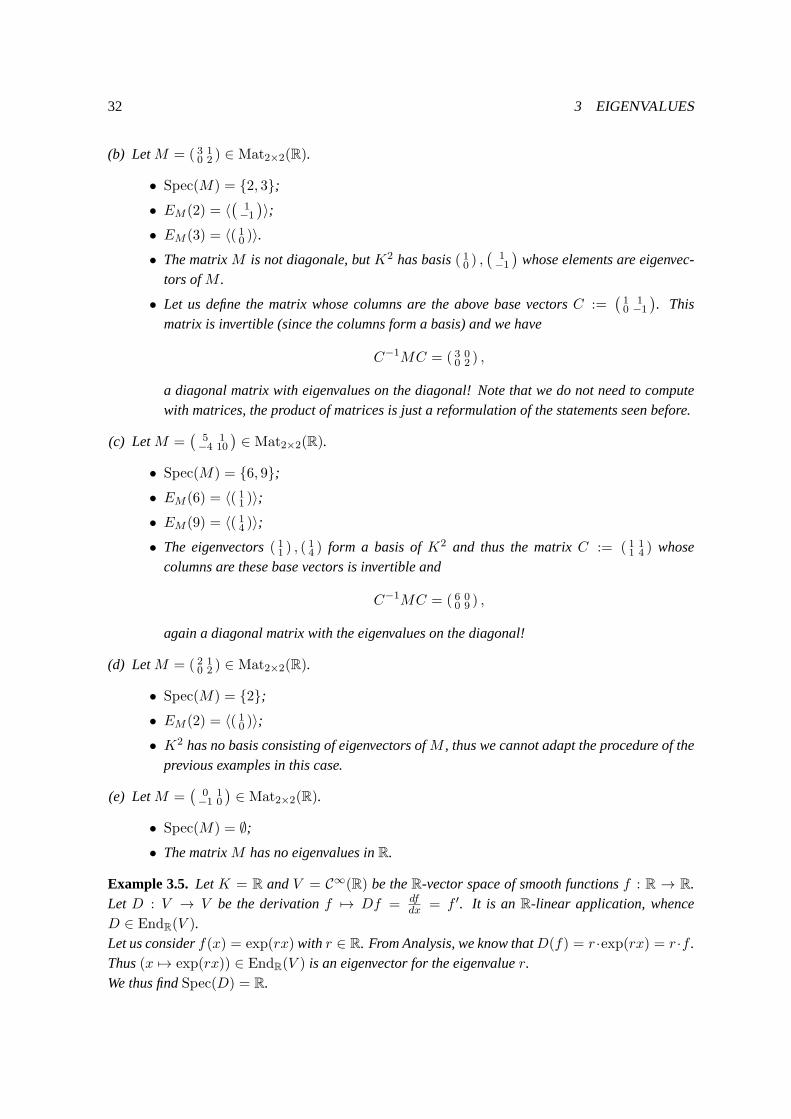
32 3 EIGENVALUES
(b) LetM = ( 3 10 2 ) ∈ Mat2×2(R).
• Spec(M) = {2, 3};
• EM (2) = 〈(
1−1
)〉;
• EM (3) = 〈( 10 )〉.• The matrixM is not diagonale, butK2 has basis( 10 ) ,
(1−1
)whose elements are eigenvec-
tors ofM .
• Let us define the matrix whose columns are the above base vectorsC :=(1 10 −1
). This
matrix is invertible (since the columns form a basis) and we have
C−1MC = ( 3 00 2 ) ,
a diagonal matrix with eigenvalues on the diagonal! Note that we do not needto computewith matrices, the product of matrices is just a reformulation of the statementsseen before.
(c) LetM =(
5 1−4 10
)∈ Mat2×2(R).
• Spec(M) = {6, 9};
• EM (6) = 〈( 11 )〉;• EM (9) = 〈( 14 )〉;• The eigenvectors( 11 ) , (
14 ) form a basis ofK2 and thus the matrixC := ( 1 1
1 4 ) whosecolumns are these base vectors is invertible and
C−1MC = ( 6 00 9 ) ,
again a diagonal matrix with the eigenvalues on the diagonal!
(d) LetM = ( 2 10 2 ) ∈ Mat2×2(R).
• Spec(M) = {2};
• EM (2) = 〈( 10 )〉;• K2 has no basis consisting of eigenvectors ofM , thus we cannot adapt the procedure of the
previous examples in this case.
(e) LetM =(
0 1−1 0
)∈ Mat2×2(R).
• Spec(M) = ∅;
• The matrixM has no eigenvalues inR.
Example 3.5. LetK = R andV = C∞(R) be theR-vector space of smooth functionsf : R → R.Let D : V → V be the derivationf 7→ Df = df
dx = f ′. It is an R-linear application, whenceD ∈ EndR(V ).Let us considerf(x) = exp(rx) with r ∈ R. From Analysis, we know thatD(f) = r ·exp(rx) = r ·f .Thus(x 7→ exp(rx)) ∈ EndR(V ) is an eigenvector for the eigenvaluer.We thus findSpec(D) = R.
33
In some examples we have met matricesM such that there is an invertible matrixC with the propertythatC−1MC is a diagonal matrix. But we have also seen examples where we could not find such amatrixC.
Definition 3.6. (a) A matrixM is said to bediagonalizableif there exists an invertible matrixC suchthatC−1MC is diagonal.
(b) LetV be aK-vector space of finite dimensionn andϕ ∈ EndK(V ). We say thatϕ is diagonal-izableif V admits aK-basis consisting of eigenvectors ofϕ.
This definition precisely expresses the idea of diagonalization mentioned before, as the followinglemma tells us. Its proof indicates how to find the matrixC (which is not unique, in general).
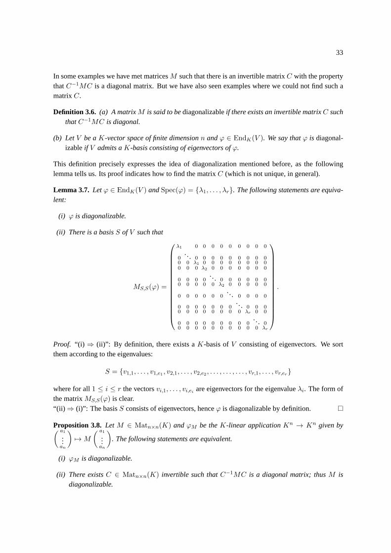
Lemma 3.7. Letϕ ∈ EndK(V ) andSpec(ϕ) = {λ1, . . . , λr}. The following statements are equiva-lent:
(i) ϕ is diagonalizable.
(ii) There is a basisS of V such that
MS,S(ϕ) =
λ1 0 0 0 0 0 0 0 0 0
0... 0 0 0 0 0 0 0 0 0
0 0 λ1 0 0 0 0 0 0 0 00 0 0 λ2 0 0 0 0 0 0 0
0 0 0 0... 0 0 0 0 0 0
0 0 0 0 0 λ2 0 0 0 0 0
0 0 0 0 0 0... 0 0 0 0
0 0 0 0 0 0 0... 0 0 0
0 0 0 0 0 0 0 0 λr 0 0
0 0 0 0 0 0 0 0 0... 0
0 0 0 0 0 0 0 0 0 0 λr
.
Proof. “(i) ⇒ (ii)”: By definition, there exists aK-basis ofV consisting of eigenvectors. We sortthem according to the eigenvalues:
S = {v1,1, . . . , v1,e1 , v2,1, . . . , v2,e2 , . . . , . . . , . . . , vr,1, . . . , vr,er}
where for all1 ≤ i ≤ r the vectorsvi,1, . . . , vi,ei are eigenvectors for the eigenvalueλi. The form ofthe matrixMS,S(ϕ) is clear.“(ii) ⇒ (i)”: The basisS consists of eigenvectors, henceϕ is diagonalizable by definition.
Proposition 3.8. LetM ∈ Matn×n(K) andϕM be theK-linear applicationKn → Kn given by( a1...an
)7→M
( a1...an
). The following statements are equivalent.
(i) ϕM is diagonalizable.
(ii) There existsC ∈ Matn×n(K) invertible such thatC−1MC is a diagonal matrix; thusM isdiagonalizable.
34 3 EIGENVALUES
Proof. “(i) ⇒ (ii)”: Let S be theK-basis ofKn which exists in view of diagonalizability ofϕM . Itsuffices to takeC to be the matrix whose columns are the elements of basisS.“(ii) ⇒ (i)”: Let ei be thei-th standard vector. It is an eigenvector for the matrixC−1MC, say witheigenvalueλi. The equalityC−1MCei = λi ·ei givesMCei = λi ·Cei, i.e.Cei is an eigenvector forthe matrixM of same eigenvalue. But,Cei is nothing but thei-th column ofC. Thus, the columnsof C form a basis ofKn consisting of eigenvectors.
The question that we are now interested in, is the following: how can we decide whetherϕ (orM ) isdiagonalizable and, if this is the case, how can we find the matrixC? In fact, it is useful to considertwo “sub-questions” individually:
• How can we computeSpec(ϕ)?
• Forλ ∈ Spec(ϕ), how can we compute the eigenspaceEϕ(λ)?
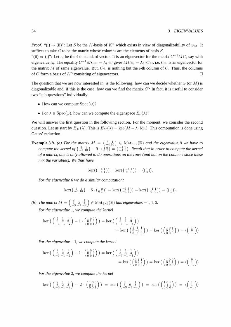
We will answer the first question in the following section. For the moment, we consider the secondquestion. Let us start byEM (λ). This isEM (λ) = ker(M −λ · idn). This computation is done usingGauss’ reduction.
Example 3.9. (a) For the matrixM =(
5 1−4 10
)∈ Mat2×2(R) and the eigenvalue9 we have to
compute the kernel of(
5 1−4 10
)− 9 · ( 1 0
0 1 ) =(−4 1−4 1
). Recall that in order to compute the kernel
of a matrix, one is only allowed to do operations on the rows (and not on the columns since thesemix the variables). We thus have
ker((−4 1−4 1
)) = ker(
(−4 10 0
)) = 〈( 14 )〉.
For the eigenvalue6 we do a similar computation:
ker((
5 1−4 10
)− 6 · ( 1 0
0 1 )) = ker((−1 1−4 4
)) = ker(
(−1 10 0
)) = 〈( 11 )〉.
(b) The matrixM =(
2 1 13 2 3−3 −1 −2
)∈ Mat3×3(R) has eigenvalues−1, 1, 2.
For the eigenvalue1, we compute the kernel
ker( ( 2 1 1
3 2 3−3 −1 −2
)− 1 ·
(1 0 00 1 00 0 1
) )= ker
( ( 1 1 13 1 3−3 −1 −3
) )
= ker( ( 1 1 1
0 −2 00 0 0
) )= ker
( ( 1 0 10 1 00 0 0
) )= 〈(
10−1
)〉
For the eigenvalue−1, we compute the kernel
ker( ( 2 1 1
3 2 3−3 −1 −2
)+ 1 ·
(1 0 00 1 00 0 1
) )= ker
( ( 3 1 13 3 3−3 −1 −1
) )
= ker( ( 3 1 1
0 2 20 0 0
) )= ker
( ( 1 0 00 1 10 0 0
) )= 〈(
01−1
)〉
For the eigenvalue2, we compute the kernel
ker( ( 2 1 1
3 2 3−3 −1 −2
)− 2 ·
(1 0 00 1 00 0 1
) )= ker
( ( 0 1 13 0 3−3 −1 −4
) )= ker
( ( 1 0 10 1 10 0 0
) )= 〈
(11−1
)〉
35
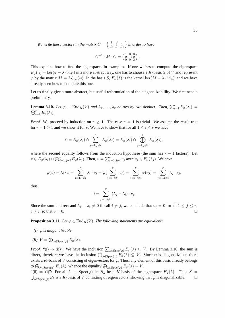
We write these vectors in the matrixC =(
1 0 10 1 1−1 −1 −1
)in order to have
C−1 ·M · C =(
1 0 00 −1 00 0 2
).
This explains how to find the eigenspaces in examples. If one wishes to compute the eigenspaceEϕ(λ) = ker(ϕ− λ · idV ) in a more abstract way, one has to choose aK-basisS of V and representϕ by the matrixM = MS,S(ϕ). In the basisS, Eϕ(λ) is the kernelker(M − λ · idn), and we havealready seen how to compute this one.
Let us finally give a more abstract, but useful reformulation of the diagonalizablility. We first need apreliminary.
Lemma 3.10. Let ϕ ∈ EndK(V ) and λ1, . . . , λr be two by two distinct. Then,∑r
i=1Eϕ(λi) =⊕ri=1Eϕ(λi).
Proof. We proceed by induction onr ≥ 1. The caser = 1 is trivial. We assume the result truefor r − 1 ≥ 1 and we show it forr. We have to show that for all1 ≤ i ≤ r we have
0 = Eϕ(λi) ∩r∑
j=1,j 6=iEϕ(λj) = Eϕ(λi) ∩
r⊕
j=1,j 6=iEϕ(λj),
where the second equality follows from the induction hypothese (the sum has r − 1 factors). Letv ∈ Eϕ(λi) ∩
⊕rj=1,j 6=iEϕ(λj). Then,v =
∑rj=1,j 6=i vj avecvj ∈ Eϕ(λj). We have
ϕ(v) = λi · v =r∑
j=1,j 6=iλi · vj = ϕ(
r∑
j=1,j 6=ivj) =
r∑
j=1,j 6=iϕ(vj) =
r∑
j=1,j 6=iλj · vj ,
thus
0 =r∑
j=1,j 6=i(λj − λi) · vj .
Since the sum is direct andλj − λi 6= 0 for all i 6= j, we conclude thatvj = 0 for all 1 ≤ j ≤ r,j 6= i, so thatv = 0.
Proposition 3.11. Letϕ ∈ EndK(V ). The following statements are equivalent:
(i) ϕ is diagonalizable.
(ii) V =⊕
λ∈Spec(ϕ)Eϕ(λ).
Proof. “(i) ⇒ (ii)”: We have the inclusion∑
λ∈Spec(ϕ)Eϕ(λ) ⊆ V . By Lemma 3.10, the sum isdirect, therefore we have the inclusion
⊕λ∈Spec(ϕ)Eϕ(λ) ⊆ V . Sinceϕ is diagonalizable, there
exists aK-basis ofV consisting of eigenvectors forϕ. Thus, any element of this basis already belongsto⊕
λ∈Spec(ϕ)Eϕ(λ), whence the equality⊕
λ∈Spec(ϕ)Eϕ(λ) = V .“(ii) ⇒ (i)”: For all λ ∈ Spec(ϕ) let Sλ be aK-basis of the eigenspaceEϕ(λ). ThusS =⋃λ∈Spec(ϕ) Sλ is aK-basis ofV consisting of eigenvectors, showing thatϕ is diagonalizable.
36 4 EXCURSION: EUCLIDEAN DIVISION AND GCD OF POLYNOMIALS
4 Excursion: euclidean division and gcd of polynomials
Goals:
• Master the euclidean division and Euclide’s algorithm;
• be able to compute the euclidean division, the gcd and a Bezout identity using Euclide’s algo-rithm.
We assume that notions of polynomials are known from highschool or otherlecture courses. Wedenote byK[X] the set of all polynomials with coefficients inK, whereX denotes the variable. Apolynomial can hence be written as finite sum
∑di=0 aiX
i with a0, . . . , ad ∈ K. We can of coursechoose any other symbol for the variable, e.g.x, T , ✷; in this case, we write
∑di=0 aix
i,∑d
i=0 aiTi,∑d
i=0 ai✷i,K[x],K[T ],K[✷], etc.
The degree of a polynomialf will be denoteddeg(f) with the conventiondeg(0) = −∞. Recall thatfor anyf, g ∈ K[X] we havedeg(fg) = deg(f)+deg(g) anddeg(f + g) ≤ max{deg(f), deg(g)}.
Definition 4.1. A polynomialf =∑d
i=0 aiXi of degreed is calledunitary if ad = 1.
A polynomialf ∈ K[X] of degree≥ 1 is calledirreducibleif it cannot be written as productf = gh
with g, h ∈ K[X] of degree≥ 1.
It is a fact that the only irreducible polynomials inC[X] are the polynomials of degree1. (Onesays thatC is algebraically closed.) Any irreducible polynomial inR[X] is either of degree1 (andtrivially, any polynomial of degree1 is irreducible), or of degree2 (there exist irreducible polynomialsof degree2, such asX2 + 1, but also reducible polynomials, such asX2 − 1 = (X − 1)(X + 1);more precisely, a polynomial of degree2 is irreducible if and only if its discriminant is negative).
Definition 4.2. A polynomialf ∈ K[X] is calleddivisor of a polynomialg ∈ K[X] if there existsq ∈ K[X] such thatg = qf . We use the notation notationf | g.
If f dividesg, we clearly havedeg(f) ≤ deg(g).For everything that will be done on polynomials in this lecture course, the euclidean division plays acentral role. We now prove its existence.
Theorem 4.3(Euclidean division). Letg =∑d
i=0 biXi ∈ K[X] be a polynomial of degreed ≥ 0.
Then, for any polynomialf ∈ K[X] there exist unique polynomialsq, r ∈ K[X] such that
f = qg + r and deg(r) < d.
We callr therestof the division.
Proof. Let f(X) =∑n
i=0 aiXi ∈ K[X] of degreen.
Existence:We prove the existence by induction onn. If n < d, we setq = 0 andr = f and we aredone. Let us therefore assumen ≥ d and that the existence is already known for all polynomials ofdegree strictly smaller thann. We set
f1(X) := f(X)− an · b−1d Xn−dg(X).
37
This is a polynomial of degree at mostn−1 since we annihilated the coefficient in front ofXn. Then,by induction hypothesis, there areq1, r1 ∈ K[X] such thatf1 = q1g + r1 anddeg(r1) < d. Thus
f(X) = f1(X) + anb−1d g(X)Xn−d = q(X)g(X) + r1(X)
whereq(X) := q1(X) + anb−1d Xn−d and we have shown the existence.
Uniqueness:Assume thatf = qg + r = q1g + r1 with q, q1, r, r1 ∈ K[X] anddeg(r), deg(r1) < d.Theng(q − q1) = r1 − r. If q = q1, thenr = r1 and we are done. Ifq 6= q1, thendeg(q − q1) ≥ 0
and we finddeg(r1− r) = deg(g(q− q1)) ≥ deg(g) = d. This is a contradiction, thusq 6= q1 cannotappear.
In the exercises, you will do euclidean divisions.
Corollary 4.4. Let f ∈ K[X] be a polynomial of degreedeg(f) ≥ 1 and leta ∈ K. Then, thefollowing statements are equivalent:
(i) f(a) = 0
(ii) (X − a) | f
Proof. (i) ⇒ (ii): Assume thatf(a) = 0 and compute the euclidean division off(X) byX − a:
f(X) = q(X)(X − a) + r
for r ∈ K (a polynomial of degree< 1). Evaluating this equality ina, gives0 = f(a) = q(a)(a −a) + r = r, and thus the rest is zero.(ii) ⇒ (i): Assume thatX − a dividesf(X). Then we havef(X) = q(X) · (X − a) for somepolynomialq ∈ K[X]. Evaluating this ina givesf(a) = q(a) · (a− a) = 0.
Proposition 4.5. Let f, g ∈ K[X] be two polynomials such thatf 6= 0. Then there exists a uniqueunitary polynomiald ∈ K[X], calledgreatest common divisorpgcd(f, g), such that
• d | f andd | g (common divisor) and
• for all e ∈ K[X] we have((e | f ande | g) ⇒ e | d) (greatestin the sense that any othercommon divisor dividesd).
Moreover, there exist polynomialsa, b ∈ K[X] such that we have aBezout relation
d = af + bg.
Proof. We show that Euclide’s algorithm gives the result.
• Preparation:We set {f0 = f, f1 = g if deg(f) ≥ deg(g),
f0 = g, f1 = f otherwise.
We also setB0 = ( 1 00 1 ).

38 4 EXCURSION: EUCLIDEAN DIVISION AND GCD OF POLYNOMIALS
• If f1 = 0, westopand setd := f0.If f1 6= 0, we do the euclidean division
f0 = f1q1 + f2 whereq1, f2 ∈ A such that(f2 = 0 or deg(f2) < deg(f1)).
We setA1 :=(−q1 1
1 0
),B1 := A1B0.
We have(f2f1
)= A1
(f1f0
)= B1
(f1f0
).
• If f2 = 0, westopand we setd := f1.If f2 6= 0, we do the euclidean division
f1 = f2q2 + f3 whereq2, f3 ∈ A such that(f3 = 0 or deg(f3) < deg(f2)).
We setA2 :=(−q2 1
1 0
),B2 := A2B1.
We have(f3f2
)= A2
(f2f1
)= B2
(f1f0
).
• If f3 = 0, westopand setd := f2.If f3 6= 0, we do the euclidean division
f2 = f3q3 + f4 whereq3, f4 ∈ A such that(f4 = 0 or deg(f4) < deg(f3)).
We setA3 :=(−q3 1
1 0
),B3 := A3B2.
We have(f4f3
)= A3
(f3f2
)= B3
(f1f0
).
• · · ·
• If fn = 0, westopand setd := fn−1.If fn 6= 0, we do the euclidean division
fn−1 = fnqn + fn+1 whereqn, fn+1 ∈ A such that(fn+1 = 0 or deg(fn+1) < deg(fn)).
We setAn :=(−qn 1
1 0
),Bn := AnBn−1.
We have(fn+1
fn
)= An
(fnfn−1
)= Bn
(f1f0
).
• · · ·
It is clear that the above algorithm (it is Euclide’s algorithm!) stops since
deg(fn) < deg(fn−1) < · · · < deg(f2) < deg(f1)
are natural numbers or−∞.Let us assume that the algorithm stops withfn = 0. Then,d = fn−1. By construction we have:
(fnfn−1
)=(0d
)= Bn−1
(f1f0
)= ( α β
r s )(f1f0
)=(αf1+βf0rf1+sf0
),

39
showingd = rf1 + sf0. (4.1)
Note that the determinant ofAi is −1 for all i, hencedet(Bn−1) = (−1)n−1. Thus the matrixC := (−1)n−1
(s −β−r α
)is the inverse ofBn−1. Therefore
(f1f0
)= CBn−1
(f1f0
)= C
(0d
)=(
d(−1)nβ
d(−1)n−1α
),
showingd | f1 andd | f0. This shows thatd is a common divisor off0 andf1. If e is any commondivisor of f0 andf1, then by Equation (4.1)e divisdesd. Finally, one dividesd, r, s by the leadingcoefficient ofd to maked unitary.If we haved1, d2 unitary gcds, thend1 dividesd2 andd2 dividesd1. As both are unitary, it followsthatd1 = d2,proving the uniqueness.
In the exercises, you will train to compute the gcd of two polynomials. We do notrequire to usematrices in order to find Bezout’s relation; it will simply suffice to “ go up” through the equalities inorder to get it.
5 Characteristic polynmial
Goals:
• Master the definition of characteristic polynomial;
• know its meaning for the computation of eigenvalues;
• be able to compute characteristic polynomials;
• know examples and be able to prove simple properties.
In Section 3 we have seen how to compute the eigenspace for a given eigenvalue. Here we will answerthe question:How to find the eigenvalues?Let us start with the main idea. Letλ ∈ K andM a square matrix. Recall
EM (λ) = ker(λ · id−M).
We have the following equivalences:
(i) λ is an eigenvalue forM .
(ii) EM (λ) 6= 0.
(iii) The matrixλ · id−M is not invertible.
(iv) det(λ · id−M) = 0.
The main idea is to considerλ as a variableX. Then the determinant ofX · id − M becomes apolynomial inK[X]. It is the characteristic polynomial. By the above equivalences, its roots areprecisely the eigenvalues ofM .
40 5 CHARACTERISTIC POLYNMIAL
Definition 5.1. • Let M ∈ Matn×n(K) be a matrix. Thecharacteristic polynomial ofM isdefined by
charpolyM (X) := det(X · idn −M
)∈ K[X].
• LetV be aK-vector space of finite dimension andϕ ∈ EndK(V ) andS aK-basis ofV . Thecharacteristic polynomial ofϕ is defined by
charpolyφ(X) := charpolyMS,S(ϕ)(X).
Remark 5.2. Information for ‘experts’: Note that the definition of characteristic polynomials usesthe determinants in the ringK[X]. That is the reason why we presented the determinants in a moregeneral way in the recall. Alternatively, one can also work in the field of rational functions overK,i.e. the field whose elements are fractions of polynomials with coefficients inK.
Lemma 5.3. LetM ∈ Matn×n(K).
(a) charpolyM (X) is a unitary polynomial of degreen.
(b) charpolyM (X) is conjugation invariant, i.e., for allN ∈ GLn(K) we have the equality
charpolyM (X) = charpolyM N−1MN(X).
Proof. (a) This is proved by induction onn. The casen = 1 is clear because the matrix is(X−m1,1),hence its determinant isX −m1,1.For the induction step, recall the notationM ′
i,j for the matrix obtained byM when deleting thei-throw and thej-th column. Assume the result is proved forn− 1. By Laplace expansion, we have
charpolyM (X) = (X −m1,1) charpolyM ′
1,1(X)−
n∑
i=2
(−1)imi,1 · det(X · id−M
)′i,1.
By hypothesis induction,charpolyM1,1(X) is a unitary polynomial of degreen − 1, hence(X −
m1,1) charpolyM1,1(X) is unitary of degreen. In the matrix
(X · id−M
)′i,1
with i 6= 1, the variableX only appearsn− 2 times. Thus in the characteristic polynomial, it can only appear to then− 2-thpower at most. Consequently,charpolyM (X) is unitary.(b) We use the multiplicativity of the determinant for the ringK[X] (Proposition 2.15).
charpolyN−1MN (X) = det(X · idn −N−1MN) = det(N−1(X · idn −M)N)
= det(N)−1 det(X · idn −M) det(N) = det(X · idn −M) = charpolyM (X).
Corollary 5.4. LetV be aK-vector space of finite dimensionn.
(a) charpolyϕ(X) is a unitary polynomial of degreen.
(b) charpolyϕ(X) is independent from the choice of the basis ofV which appears in its definition.
41
Proof. (a) Lemma 5.3 (a).(b) Let S andT be two basis ofV . The statement follows from Lemma 5.3 (b) and the equalityMT,T (ϕ) = C−1
S,T ◦MS,S(ϕ) ◦ CS,T .
We reconsider the examples of Section 3.
Example 5.5. (a) LetM =
(3 0
0 2
)∈ Mat2×2(R). We find
charpolyM (X) = (X − 3)(X − 2).
(It is important to know the factorization in irreducible polynomials of the characteristic polyno-mial. Thus it is useless to write it asX2 − 5X + 6.)
(b) LetM =
(3 1
0 2
)∈ Mat2×2(R). We find once again
charpolyM (X) = (X − 3)(X − 2).
(c) LetM =
(5 1
−4 10
)∈ Mat2×2(R). We find
charpolyM (X) = (X − 5)(X − 10) + 4 = (X − 6)(X − 9).
Note that in order to simplify the computation, Lemma 5.3 (b) allows us to use the conjugate
matrix
(1 1
1 4
)−1(5 1
−4 10
)(1 1
1 4
)=
(6 0
0 9
)for the computation of the characteristic
polynomial, thus one can immediately write the factorization in linear factors (in general, thiswill not be possible).
(d) LetM =
(2 1
0 2
)∈ Mat2×2(R). We find
charpolyM (X) = (X − 2)2,
a polynomial with a double root.
(e) LetM =
(0 1
−1 0
)∈ Mat2×2(R). We find
charpolyM (X) = X2 + 1,
a polynomial that does not factor in linear factors inR[X].
(f) LetM =(
2 1 13 2 3−3 −1 −2
)∈ Mat3×3(R). For the characteristic polynomial, we compute the deter-
minant∣∣∣∣X−2 −1 −1−3 X−2 −33 1 X+2
∣∣∣∣ = (X − 2) ·∣∣X−2 −3
1 X+2
∣∣+ 3 ·∣∣−1 −1
1 X+2
∣∣+ 3 ·∣∣ −1 −1X−2 −3
∣∣
= (X − 2)((X − 2)(X + 2) + 3
)+ 3 ·
(− (X + 2) + 1
)+ 3 ·
(3 + (X − 2)
)
= (X − 2)(X2 − 1) = (X − 2)(X − 1)(X + 1)
42 5 CHARACTERISTIC POLYNMIAL
Proposition 5.6. (a) ForM ∈ Matn×n(K) we have
Spec(M) = {a ∈ K | charpolyM (a) = 0} = {a ∈ K | (X − a) | charpolyM (X)}.
(b) Forϕ ∈ EndK(V ) with aK-vector spaceV of finite dimension, we have
Spec(ϕ) = {a ∈ K | charpolyϕ(a) = 0} = {a ∈ K | (X − a) | charpolyϕ(X)}.
Proof. It suffices to prove (a). The first equality follows from (witha ∈ K):
a ∈ Spec(M) ⇔ ker(a · idn −M) 6= 0 ⇔ det(a · idn −M)︸ ︷︷ ︸=charpolyM (a)
= 0 ⇔ charpolyM (a) = 0.
The second equality is just the fact thata ∈ K is a root of a polynomialf if and only if (X − a)|f(Corollary 4.4).
We have thus identified the eigenvalues with the roots of the characteristic polynomial. This answersour question in the beginning:In order to compute the eigenvalues of a matrix, compute its char-acteristic polynomial and find its roots.But the characteristic polynomial has another important property that was discovered by Cayley andHamilton. We first need to introduce some terminology.
Definition 5.7. (a) LetM ∈ Matn×n(K) be a matrix. Iff(X) =∑d
i=0 aiXi ∈ K[X] is a polyno-
mial, then we setf(M) :=∑d
i=0 aiMi ∈ Matn×n(K). Note:M0 = idn.
(b) Letϕ ∈ EndK(V ) be an endomorphism of aK-vector spaceV . If f(X) =∑d
i=0 aiXi ∈ K[X]
is a polynomial, then we setf(ϕ) :=∑d
i=0 aiϕi, which is still an endomorphism inEndK(V ).
Be careful:ϕi = ϕ ◦ ϕ ◦ · · · ◦ ϕ︸ ︷︷ ︸i times
etϕ0 = idV .
Definition-Lemma 5.8 (For mathematicians only). (a) The application “evaluation”
evM : K[X] → Matn×n(K), f(X) 7→ f(M)
is a ring homomorphism (even a homomorphism ofK-algebras).
(b) The application “evaluation”
evϕ : K[X] → EndK(V ), f(X) 7→ f(ϕ)
is a ring homomorphism (even a homomorphism ofK-algebras).
Proof. Easy computations.
Theorem 5.9(Cayley-Hamilton). LetM ∈ Matn×n(K). Then,
charpolyM (M) = 0n ∈ Matn×n(K).
43
Proof. The trick is to use adjoint matrices. InMatn×n(K[X]) we have
(X · idn −M)# · (X · idn −M) = det(X · idn −M) · idn déf= charpolyM (X) · idn. (5.2)
The idea of the proof is very simple: if one replacesX byM in (5.2), one obtains0, since on the lefthand side we have the factor(M ·idn−M) =M−M = 0. The problem is that inMatn×n(K[X]),Xappears in the coefficients of the matrices, and we are certainly not allowedto replace a coefficient of amatrix by a matrix. What we do is to write a matrix whose coefficients are polynomialsas polynomialwhose coefficients are matrices:
∑dk=0 a1,1,kX
k · · · ∑dk=0 a1,n,kX
k
.... . .
...∑dk=0 an,1,kX
k · · · ∑dk=0 an,n,kX
k
=
d∑
k=0
a1,1,k · · · a1,n,k
.... . .
...an,1,k · · · an,n,k
·Xk · idn.
Having done this, one would have to show that the evaluation of this polynomialwith matrix coeffi-cients in a matrix gives rise to a ring homomorphism. Unfortunately, the matrix ring isnot commuta-tive, hence the developed theory does not apply. The proof that we give avoids this problem by doinga comparison of the coefficients instead of an evaluation, but is based on the same idea.The definition of adjoint matrix shows that the largest power ofX that can appear in a coefficient ofthe matrix(X · idn−M)# isn−1. As indicated above, we can hence write this matrix as polynomialof degreen− 1 with coefficients inMatn×n(K):
(X · idn −M)# =n−1∑
i=0
BiXi with Bi ∈ Matn×n(K).
We writecharpolyM (X) =∑n
i=0 aiXi (oùan = 1) and consider Equation (5.2) inMatn×n(K):
charpolyM (X) · idn =n∑
i=0
ai · idn ·Xi =( n−1∑
i=0
BiXi)(X · idn −M)
=n−1∑
i=0
(BiXi+1 −BiMXi) = −B0M +
n−1∑
i=1
(Bi−1 −BiM)Xi +Bn−1Xn.
We compare the coefficients (still matrices!) to obtain
a0 · idn = −B0M, ai · idn = Bi−1 −BiM for 1 ≤ i ≤ n− 1 and Bn−1 = idn.
This comparision of coefficients allows us to continue with our calculations inMatn×n(K) in orderto obtaincharpolyM (M) = 0n as follows:
charpolyM (M) · idn =n∑
i=0
ai ·M i = −B0M +n−1∑
i=1
(Bi−1 −BiM)M i +Bn−1Mn
= −B0M +B0M −B1M2 +B1M
2 −B2M3 +B2M
3 − · · · −Bn−1Mn +Bn−1M
n = 0n.
44 6 MINIMAL POLYNOMIAL
The theorem of Cayley-Hamilton is still true if one replaces the matrixM by an endomorphismϕ ∈EndK(V ).
Theorem 5.10(Cayley-Hamilton for endomorphisms). LetV be aK-vector space of finite dimensionandϕ ∈ EndK(ϕ). Then,charpolyϕ(ϕ) = 0 ∈ EndK(V ).
Proof. By definition we have,charpolyϕ(X) = charpolyMS,S(ϕ)(X) and by Theorem 5.9
0 = charpolyMS,S(ϕ)(MS,S(ϕ)) =MS,S(charpolyMS,S(ϕ)(ϕ)) =MS,S(charpolyϕ(ϕ)),
thuscharpolyϕ(ϕ) = 0. This computation is based onMS,S(ϕi) =
(MS,S(ϕ)
)i(see exercises)
6 Minimal polynomial
Goals:
• Master the definition of minimal polynomial;
• know its meaning for the computation of eigenvalues;
• know how to compute minimal polynomials;
• know examples and be able to prove simple properties.
Beside the characteristic polynomial, we will also introduce theminimal polynomial.
Definition-Lemma 6.1. LetM ∈ Matn×n(K) be a matrix.
(a) There exists a unique unitary polynomialmipoM (X) ∈ K[X] of minimal degree with the prop-ertymipoM (M) = 0n. This polynomial is called theminimal polynomial ofM .
(b) Any polynomialf ∈ K[X] with the propertyf(M) = 0n is a multiple ofmipoM (X).
(c) For any invertible matrixN ∈ Matn×n(K), we havemipoN−1MN (X) = mipoM (X).
(d) Letϕ ∈ EndK(V ) for aK-vector spaceV of finite dimension withK-basisS. We set
mipoϕ(X) := mipoMS,S(ϕ)(X)
and call it minimal polynomial ofϕ. This polynomial is independent from the choice of thebasisS.
Proof. (a,b) By Theorem of Cayley-Hamilton 5.9 there exists a polynomial0 6= f ∈ K[X] thatannihilatesM . Let us now consider the set of such polynomials
E = {f ∈ K[X] | f 6= 0 andf(M) = 0}.
We choose unitaryg ∈ E of minimal degree among the elements ofE.
45
We will use the euclidean division to show the uniqueness and (b). Letf ∈ E. We thus haveq, r ∈ K[X] such thatr = 0 or deg(r) < deg(g) and
f = qg + r,
which implies
0 = f(M) = q(M)g(M) + r(M) = q(M) · 0 + r(M) = r(M).
Consequently, letr = 0, let r ∈ E. This last possibility is excluded as the degree ofr is strictlysmaller that the degree ofg which is minimal. The fact thatr = 0 meansf = qg, thus any otherpolynomial ofE is a multiple ofg. This also implies the uniqueness: iff has the same degree thangand is also unitary, thenf = g.(c) It suffices to note(N−1MN)i = N−1M iN , hence for allf ∈ K[X]
f(N−1MN) = N−1f(M)N = 0n ⇔ f(M) = 0n.
(d) The independence of the basis choice is a consequence of (c) andthe equalityMT,T (ϕ) = C−1S,T ◦
MS,S(ϕ) ◦ CS,T for any other basisT .
Proposition 6.2. LetV be aK-vector space of finite dimension andϕ ∈ EndK(V ). Then,Spec(ϕ) ={a ∈ K | (X − a) | mipoϕ(X)} = {a ∈ K | mipoϕ(a) = 0}.
Clearly, the same statement holds for matricesM ∈ Matn×n(K). Compare this proposition to Propo-sition 5.6.
Proof. The second equality is clear (same argument as in the proof of Proposition 5.6). To see thefirst equality, first assume that(X − a) ∤ mipoϕ(X). From this we deduce that the gcd of(X − a)
andmipoϕ(X) is 1, which allows us (by Euclide/Bézout algorithm) to findb, c ∈ K[X] such that1 = b(X)(X − a) + c(X)mipoϕ(X). Let nowv ∈ V t.q.ϕ(v) = av. We have
v = idV v = b(ϕ)(ϕ(v)− av) + c(ϕ)mipoϕ(ϕ)v = 0 + 0 = 0,
hencea 6∈ Spec(ϕ).Assume now that(X − a) | mipoϕ(X) which allows us to writemipoϕ(X) = (X − a)g(X) forsomeg ∈ K[X]. Since the degree ofg is strictly smaller than the degree ofmipoϕ(X), there has tobe av ∈ V such thatw := g(ϕ)v 6= 0 (otherwise, the minimal polynomialmipoϕ(X) would be adivisor ofg(X) which is impossible). We thus have
(ϕ− a)w = mipoϕ(ϕ)v = 0,
hencea ∈ Spec(ϕ).
It is useful to observe that Propositions 5.6 and 6.2 state thatcharpolyϕ(X) andmipoϕ(X) have thesame factors of degree1. Moreover, the characteristic polynomialcharpolyϕ(X) is always a multipleof the minimal polynomialmipoϕ(X), by the theorem of Cayley-Hamilton, as we will now see.
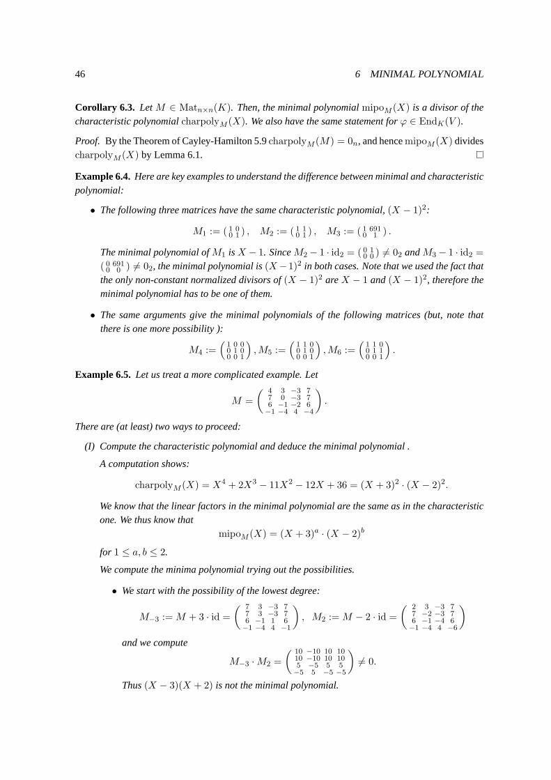
46 6 MINIMAL POLYNOMIAL
Corollary 6.3. LetM ∈ Matn×n(K). Then, the minimal polynomialmipoM (X) is a divisor of thecharacteristic polynomialcharpolyM (X). We also have the same statement forϕ ∈ EndK(V ).
Proof. By the Theorem of Cayley-Hamilton 5.9charpolyM (M) = 0n, and hencemipoM (X) dividescharpolyM (X) by Lemma 6.1.
Example 6.4.Here are key examples to understand the difference between minimal andcharacteristicpolynomial:
• The following three matrices have the same characteristic polynomial,(X − 1)2:
M1 := ( 1 00 1 ) , M2 := ( 1 1
0 1 ) , M3 := ( 1 6910 1 ) .
The minimal polynomial ofM1 isX − 1. SinceM2 − 1 · id2 = ( 0 10 0 ) 6= 02 andM3 − 1 · id2 =
( 0 6910 0 ) 6= 02, the minimal polynomial is(X−1)2 in both cases. Note that we used the fact that
the only non-constant normalized divisors of(X − 1)2 areX − 1 and(X − 1)2, therefore theminimal polynomial has to be one of them.
• The same arguments give the minimal polynomials of the following matrices (but, note thatthere is one more possibility ):
M4 :=(
1 0 00 1 00 0 1
),M5 :=
(1 1 00 1 00 0 1
),M6 :=
(1 1 00 1 10 0 1
).
Example 6.5. Let us treat a more complicated example. Let
M =
( 4 3 −3 77 0 −3 76 −1 −2 6−1 −4 4 −4
).
There are (at least) two ways to proceed:
(I) Compute the characteristic polynomial and deduce the minimal polynomial .
A computation shows:
charpolyM (X) = X4 + 2X3 − 11X2 − 12X + 36 = (X + 3)2 · (X − 2)2.
We know that the linear factors in the minimal polynomial are the same as in the characteristicone. We thus know that
mipoM (X) = (X + 3)a · (X − 2)b
for 1 ≤ a, b ≤ 2.
We compute the minima polynomial trying out the possibilities.
• We start with the possibility of the lowest degree:
M−3 :=M + 3 · id =
( 7 3 −3 77 3 −3 76 −1 1 6−1 −4 4 −1
), M2 :=M − 2 · id =
( 2 3 −3 77 −2 −3 76 −1 −4 6−1 −4 4 −6
)
and we compute
M−3 ·M2 =
( 10 −10 10 1010 −10 10 105 −5 5 5−5 5 −5 −5
)6= 0.
Thus(X − 3)(X + 2) is not the minimal polynomial.
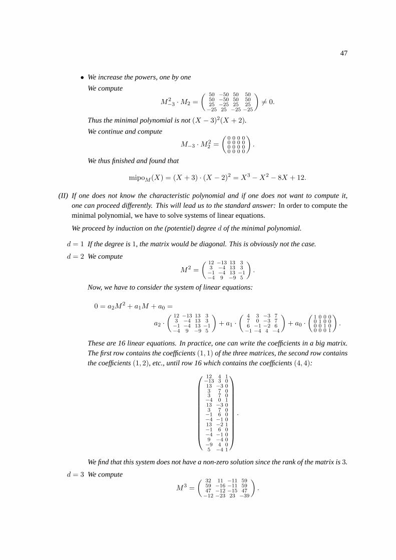
47
• We increase the powers, one by one
We compute
M2−3 ·M2 =
( 50 −50 50 5050 −50 50 5025 −25 25 25−25 25 −25 −25
)6= 0.
Thus the minimal polynomial is not(X − 3)2(X + 2).
We continue and compute
M−3 ·M22 =
(0 0 0 00 0 0 00 0 0 00 0 0 0
).
We thus finished and found that
mipoM (X) = (X + 3) · (X − 2)2 = X3 −X2 − 8X + 12.
(II) If one does not know the characteristic polynomial and if one doesnot want to compute it,one can proceed differently. This will lead us to the standard answer:In order to compute theminimal polynomial, we have to solve systems of linear equations.
We proceed by induction on the (potentiel) degreed of the minimal polynomial.
d = 1 If the degree is1, the matrix would be diagonal. This is obviously not the case.
d = 2 We compute
M2 =
( 12 −13 13 33 −4 13 3−1 −4 13 −1−4 9 −9 5
).
Now, we have to consider the system of linear equations:
0 = a2M2 + a1M + a0 =
a2 ·( 12 −13 13 3
3 −4 13 3−1 −4 13 −1−4 9 −9 5
)+ a1 ·
( 4 3 −3 77 0 −3 76 −1 −2 6−1 −4 4 −4
)+ a0 ·
(1 0 0 00 1 0 00 0 1 00 0 0 1
).
These are 16 linear equations. In practice, one can write the coefficientsin a big matrix.The first row contains the coefficients(1, 1) of the three matrices, the second row containsthe coefficients(1, 2), etc., until row 16 which contains the coefficients(4, 4):
12 4 1−13 3 013 −3 03 7 03 7 0−4 0 113 −3 03 7 0−1 6 0−4 −1 013 −2 1−1 6 0−4 −1 09 −4 0−9 4 05 −4 1
.
We find that this system does not have a non-zero solution since the rank of the matrix is3.
d = 3 We compute
M3 =
( 32 11 −11 5959 −16 −11 5947 −12 −15 47−12 −23 23 −39
).
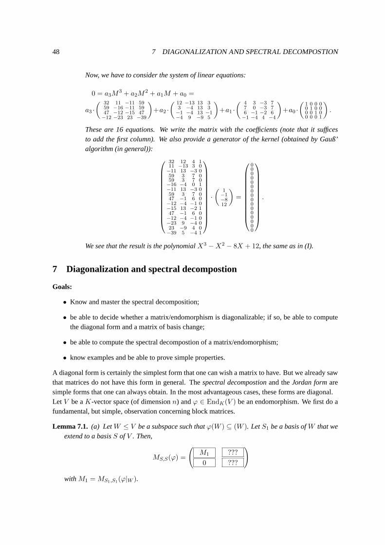
48 7 DIAGONALIZATION AND SPECTRAL DECOMPOSTION
Now, we have to consider the system of linear equations:
0 = a3M3 + a2M
2 + a1M + a0 =
a3 ·( 32 11 −11 59
59 −16 −11 5947 −12 −15 47−12 −23 23 −39
)+a2 ·
( 12 −13 13 33 −4 13 3−1 −4 13 −1−4 9 −9 5
)+a1 ·
( 4 3 −3 77 0 −3 76 −1 −2 6−1 −4 4 −4
)+a0 ·
(1 0 0 00 1 0 00 0 1 00 0 0 1
).
These are 16 equations. We write the matrix with the coefficients (note that it sufficesto add the first column). We also provide a generator of the kernel (obtained by Gauß’algorithm (in general)):
32 12 4 111 −13 3 0−11 13 −3 059 3 7 059 3 7 0−16 −4 0 1−11 13 −3 059 3 7 047 −1 6 0−12 −4 −1 0−15 13 −2 147 −1 6 0−12 −4 −1 0−23 9 −4 023 −9 4 0−39 5 −4 1
·(
1−1−812
)=
0000000000000000
.
We see that the result is the polynomialX3 −X2 − 8X + 12, the same as in (I).
7 Diagonalization and spectral decompostion
Goals:
• Know and master the spectral decomposition;
• be able to decide whether a matrix/endomorphism is diagonalizable; if so, be able to computethe diagonal form and a matrix of basis change;
• be able to compute the spectral decompostion of a matrix/endomorphism;
• know examples and be able to prove simple properties.
A diagonal form is certainly the simplest form that one can wish a matrix to have. But we already sawthat matrices do not have this form in general. Thespectral decompostionand theJordan formaresimple forms that one can always obtain. In the most advantageous cases,these forms are diagonal.Let V be aK-vector space (of dimensionn) andϕ ∈ EndK(V ) be an endomorphism. We first do afundamental, but simple, observation concerning block matrices.
Lemma 7.1. (a) LetW ≤ V be a subspace such thatϕ(W ) ⊆ (W ). LetS1 be a basis ofW that weextend to a basisS of V . Then,
MS,S(ϕ) =
(M1 ???
0 ???
)
withM1 =MS1,S1(ϕ|W ).

49
(b) LetV =W1⊕W2 be such thatϕ(Wi) ⊆Wi for i = 1, 2. LetSi be aK-basis ofWi for i = 1, 2;hence,S = S1 ∪ S2 is aK-basis ofV . Then,
MS,S(ϕ) =
(M1 0
0 M2
)
withM1 =MS1,S1(ϕ|W1) andM2 =MS2,S2(ϕ|W2).
Proof. It suffices to apply the rules to write the matrixMS,S(ϕ).
We will continue by a lemma.
Lemma 7.2. Letϕ ∈ EndK(V ).
(a) Letf ∈ K[X] andW := ker(f(ϕ)). Then,W is a subspace ofV that is stable underϕ, i.e. forall w ∈ W we haveϕ(w) ∈ W . This allows us to restrictϕ àW ; we will denote the restrictedmap byϕ|W :W →W .
(b) Letf, g ∈ K[X] be two coprime polynomials, i.e.:pgcd(f(X), g(X)) = 1. Then,
ker(f(ϕ) · g(ϕ))︸ ︷︷ ︸=:W
= ker(f(ϕ))︸ ︷︷ ︸=:W1
⊕ ker(g(ϕ))︸ ︷︷ ︸=:W2
.
Before the proof, a brief word about the notation:f(ϕ) is aK-linear applicationV → V , then onecan apply it to a vectorv ∈ V . Our notation for this is:f(ϕ)(v) or f(ϕ)v. Note the different rolesof the two pairs of parenthesis in the first expression. One could also write(f(ϕ))(v), but I find thisnotation a bit cumbersome.
Proof. (a) The kernel of anyK-linear application is a subspace. Writef(X) =∑d
i=0 aiXi. Let then
w ∈W , i.e.f(ϕ)w =∑d
i=0 aiϕi(w) = 0. We compute
f(ϕ)(ϕ(w)) =d∑
i=0
aiϕi(ϕ(w)) =
d∑
i=0
aiϕi+1(w) = ϕ
( d∑
i=0
aiϕi(w)
)= ϕ(0) = 0.
(b) It is clear thatW1 ⊆W andW2 ⊆W , whenceW1 +W2 ⊆W . We have to prove that
• W1 ∩W2 = 0 (the zeroK-vector space) and
• W1 +W2 =W .
SinceK[X] is a euclidean ring, we can use Euclide’s algorithm (Bézout) to obtain two other polyno-mialsa, b ∈ K[X] such that1 = a(X)f(X) + b(X)g(X). First considerw ∈W1 ∩W2. Then
w = idV (w) = a(ϕ)f(ϕ)w + b(ϕ)g(ϕ)w = 0 + 0 = 0,
which proves the first point. For the second, letw ∈W . The equation that we used reads
w = w2 + w1 with w2 := a(ϕ)f(ϕ)w andw1 := b(ϕ)g(ϕ)w.

50 7 DIAGONALIZATION AND SPECTRAL DECOMPOSTION
But, we havef(ϕ)(w1) = b(ϕ)f(ϕ)g(ϕ)w = b(ϕ)0 = 0 ⇒ w1 ∈W1
andg(ϕ)(w2) = a(ϕ)f(ϕ)g(ϕ)w = a(ϕ)0 = 0 ⇒ w2 ∈W2,
which concludes the proof.
Theorem 7.3(Spectral decomposition). Letϕ ∈ EndK(V ) be an endomorphism with minimal poly-nomialmipoϕ(X) = fe11 (X) · fe22 (X) · . . . · ferr (X) where the polynomialsfi(X) are irreducible(they are therefore prime elements in the principal ringK[X]) and coprime, i.e.pgcd(fi, fj) = 1 forall 1 ≤ i < j ≤ n (if one chooses thefi’s monic, then the condition is equivalent to saying that thepolynomials are all distinct). SetWi := ker(feii (ϕ)). Then the following statements hold.
(a) V =⊕r
i=1Wi.
(b) If one chooses a basisSi of the subspaceWi for 1 ≤ i ≤ r, thenS = S1 ∪ S2 ∪ · · · ∪ Sr is abasis ofW for which we have:
MS,S(ϕ) =
M1 0 0 . . . 0
0 M2 0 . . . 0...
. . . . .....
0 . . . 0 Mr−1 0
0 . . . 0 0 Mr
withMi :=MSi,Si(ϕ|Wi
) for 1 ≤ i ≤ r.
Proof. (a) follows from Lemma 7.2 (b) by induction.(b) is clear: Write the matrix with these rules in order to obtain this form. Note that the blocks outsidethe diagonal are zero sinceϕ(Wi) ⊆Wi.
The most important case is whenfi(X) = X − ai with ai 6= aj for i 6= j (which implies that thefi are irreducible and distinct). The spectral decomposition is in fact only a (decisive!) step towardsJordan reduction. In the next proposition we will also see its importance fordiagonalization. For themoment we illustrate the effect of the spectral decomposition by an example. Before this, it can beuseful to recall how one applies the results for linear applicationsϕ to matrices.
Remark 7.4. LetM ∈ Matn×n(K). One can apply the spectral decompostion toM as follwos. For
the canonical basisB := (
100...00
,
010...00
, . . . ,
000...01
) the matrixM describes aK-linear applica-
tionϕ = ϕM and one hasM =MB,B(ϕ).The spectral decomposition gives us a basisS. LetC := MB,S(id) be the matrix of basis changebetweenS and the canonical basis. Then, we have
MS,S(ϕ) = C−1MC.
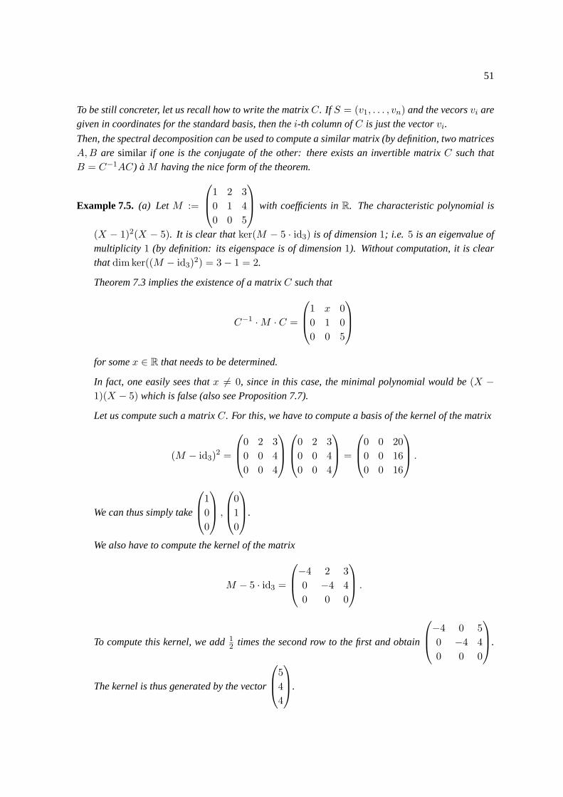
51
To be still concreter, let us recall how to write the matrixC. If S = (v1, . . . , vn) and the vecorsvi aregiven in coordinates for the standard basis, then thei-th column ofC is just the vectorvi.
Then, the spectral decomposition can be used to compute a similar matrix (by definition, two matricesA,B are similar if one is the conjugate of the other: there exists an invertible matrixC such thatB = C−1AC) àM having the nice form of the theorem.
Example 7.5. (a) LetM :=
1 2 3
0 1 4
0 0 5
with coefficients inR. The characteristic polynomial is
(X − 1)2(X − 5). It is clear thatker(M − 5 · id3) is of dimension1; i.e. 5 is an eigenvalue ofmultiplicity 1 (by definition: its eigenspace is of dimension1). Without computation, it is clearthatdimker((M − id3)
2) = 3− 1 = 2.
Theorem 7.3 implies the existence of a matrixC such that
C−1 ·M · C =
1 x 0
0 1 0
0 0 5
for somex ∈ R that needs to be determined.
In fact, one easily sees thatx 6= 0, since in this case, the minimal polynomial would be(X −1)(X − 5) which is false (also see Proposition 7.7).
Let us compute such a matrixC. For this, we have to compute a basis of the kernel of the matrix
(M − id3)2 =
0 2 3
0 0 4
0 0 4
0 2 3
0 0 4
0 0 4
=
0 0 20
0 0 16
0 0 16
.
We can thus simply take
1
0
0
,
0
1
0
.
We also have to compute the kernel of the matrix
M − 5 · id3 =
−4 2 3
0 −4 4
0 0 0
.
To compute this kernel, we add12 times the second row to the first and obtain
−4 0 5
0 −4 4
0 0 0
.
The kernel is thus generated by the vector
5
4
4
.
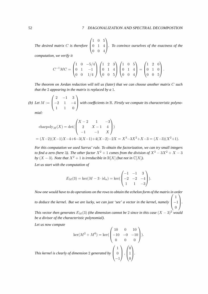
52 7 DIAGONALIZATION AND SPECTRAL DECOMPOSTION
The desired matrixC is therefore
1 0 5
0 1 4
0 0 4
. To convince ourselves of the exactness of the
computation, we verify it
C−1MC =
1 0 −5/4
0 1 −1
0 0 1/4
1 2 3
0 1 4
0 0 5
1 0 5
0 1 4
0 0 4
=
1 2 0
0 1 0
0 0 5
.
The theorem on Jordan reduction will tell us (later) that we can choose another matrixC suchthat the2 appearing in the matrix is replaced by a1.
(b) LetM :=
2 −1 3
−2 1 −4
1 1 0
with coefficients inR. Firstly we compute its characteristic polyno-
mial:
charpolyM (X) = det(
X − 2 1 −3
2 X − 1 4
−1 −1 X
)
= (X−2)(X−1)X−4+6−3(X−1)+4(X−2)−2X = X3−3X2+X−3 = (X−3)(X2+1).
For this computation we used Sarrus’ rule. To obtain the factorization, we can try small integersto find a zero (here3). The other factorX2 + 1 comes from the division ofX3 − 3X2 +X − 3
by (X − 3). Note thatX2 + 1 is irreducible inR[X] (but not inC[X]).
Let us start with the computation of
EM (3) = ker(M − 3 · idn) = ker(
−1 −1 3
−2 −2 −4
1 1 −3
).
Now one would have to do operations on the rows to obtain the echelon form ofthe matrix in order
to deduce the kernel. But we are lucky, we can just ‘see’ a vector in the kernel, namely
1
−1
0
.
This vector then generatesEM (3) (the dimension cannot be2 since in this case(X − 3)2 wouldbe a divisor of the characteristic polynomial).
Let us now compute
ker(M2 +M0) = ker(
10 0 10
−10 −0 −10
0 0 0
).
This kernel is clearly of dimension2 generated by
1
0
−1
,
0
1
0
.
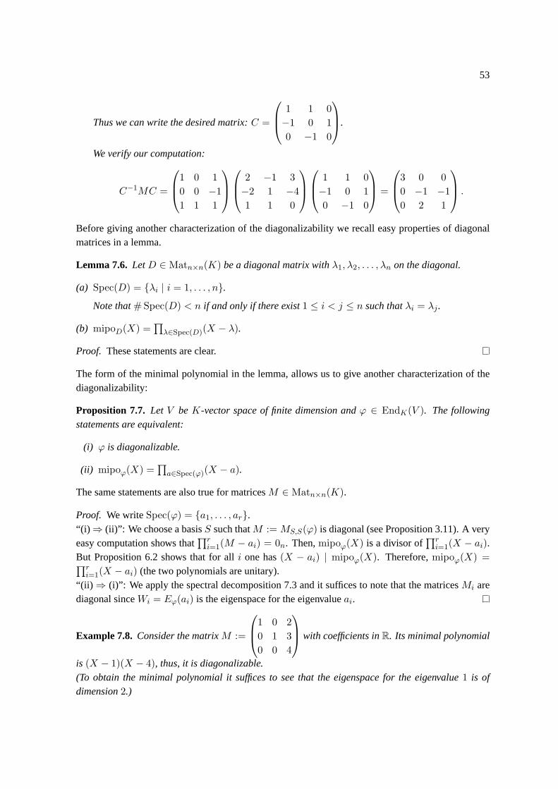
53
Thus we can write the desired matrix:C =
1 1 0
−1 0 1
0 −1 0
.
We verify our computation:
C−1MC =
1 0 1
0 0 −1
1 1 1
2 −1 3
−2 1 −4
1 1 0
1 1 0
−1 0 1
0 −1 0
=
3 0 0
0 −1 −1
0 2 1
.
Before giving another characterization of the diagonalizability we recall easy properties of diagonalmatrices in a lemma.
Lemma 7.6. LetD ∈ Matn×n(K) be a diagonal matrix withλ1, λ2, . . . , λn on the diagonal.
(a) Spec(D) = {λi | i = 1, . . . , n}.
Note that#Spec(D) < n if and only if there exist1 ≤ i < j ≤ n such thatλi = λj .
(b) mipoD(X) =∏λ∈Spec(D)(X − λ).
Proof. These statements are clear.
The form of the minimal polynomial in the lemma, allows us to give another characterization of thediagonalizability:
Proposition 7.7. Let V beK-vector space of finite dimension andϕ ∈ EndK(V ). The followingstatements are equivalent:
(i) ϕ is diagonalizable.
(ii) mipoϕ(X) =∏a∈Spec(ϕ)(X − a).
The same statements are also true for matricesM ∈ Matn×n(K).
Proof. We writeSpec(ϕ) = {a1, . . . , ar}.“(i) ⇒ (ii)”: We choose a basisS such thatM :=MS,S(ϕ) is diagonal (see Proposition 3.11). A veryeasy computation shows that
∏ri=1(M − ai) = 0n. Then,mipoϕ(X) is a divisor of
∏ri=1(X − ai).
But Proposition 6.2 shows that for alli one has(X − ai) | mipoϕ(X). Therefore,mipoϕ(X) =∏ri=1(X − ai) (the two polynomials are unitary).
“(ii) ⇒ (i)”: We apply the spectral decomposition 7.3 and it suffices to note that the matricesMi arediagonal sinceWi = Eϕ(ai) is the eigenspace for the eigenvalueai.
Example 7.8. Consider the matrixM :=
1 0 2
0 1 3
0 0 4
with coefficients inR. Its minimal polynomial
is (X − 1)(X − 4), thus, it is diagonalizable.(To obtain the minimal polynomial it suffices to see that the eigenspace for the eigenvalue1 is ofdimension2.)
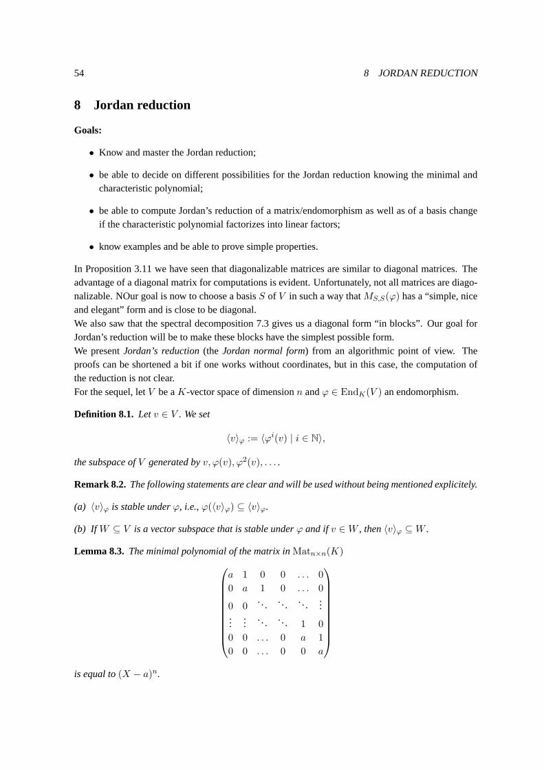
54 8 JORDAN REDUCTION
8 Jordan reduction
Goals:
• Know and master the Jordan reduction;
• be able to decide on different possibilities for the Jordan reduction knowing the minimal andcharacteristic polynomial;
• be able to compute Jordan’s reduction of a matrix/endomorphism as well as ofa basis changeif the characteristic polynomial factorizes into linear factors;
• know examples and be able to prove simple properties.
In Proposition 3.11 we have seen that diagonalizable matrices are similar to diagonal matrices. Theadvantage of a diagonal matrix for computations is evident. Unfortunately, not all matrices are diago-nalizable. NOur goal is now to choose a basisS of V in such a way thatMS,S(ϕ) has a “simple, niceand elegant” form and is close to be diagonal.We also saw that the spectral decomposition 7.3 gives us a diagonal form “in blocks”. Our goal forJordan’s reduction will be to make these blocks have the simplest possible form.We presentJordan’s reduction(the Jordan normal form) from an algorithmic point of view. Theproofs can be shortened a bit if one works without coordinates, but in this case, the computation ofthe reduction is not clear.For the sequel, letV be aK-vector space of dimensionn andϕ ∈ EndK(V ) an endomorphism.
Definition 8.1. Letv ∈ V . We set
〈v〉ϕ := 〈ϕi(v) | i ∈ N〉,
the subspace ofV generated byv, ϕ(v), ϕ2(v), . . . .
Remark 8.2. The following statements are clear and will be used without being mentioned explicitely.
(a) 〈v〉ϕ is stable underϕ, i.e.,ϕ(〈v〉ϕ) ⊆ 〈v〉ϕ.
(b) If W ⊆ V is a vector subspace that is stable underϕ and ifv ∈W , then〈v〉ϕ ⊆W .
Lemma 8.3. The minimal polynomial of the matrix inMatn×n(K)
a 1 0 0 . . . 0
0 a 1 0 . . . 0
0 0. .. .. . . . .
......
.... .. .. . 1 0
0 0 . . . 0 a 1
0 0 . . . 0 0 a
is equal to(X − a)n.
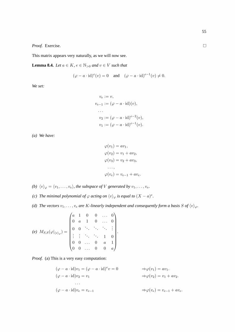
55
Proof. Exercise.
This matrix appears very naturally, as we will now see.
Lemma 8.4. Leta ∈ K, e ∈ N>0 andv ∈ V such that
(ϕ− a · id)e(v) = 0 and (ϕ− a · id)e−1(v) 6= 0.
We set:
ve := v,
ve−1 := (ϕ− a · id)(v),. . .
v2 := (ϕ− a · id)e−2(v),
v1 := (ϕ− a · id)e−1(v).
(a) We have:
ϕ(v1) = av1,
ϕ(v2) = v1 + av2,
ϕ(v3) = v2 + av3,
. . . ,
ϕ(ve) = ve−1 + ave.
(b) 〈v〉ϕ = 〈v1, . . . , ve〉, the subspace ofV generated byv1, . . . , ve.
(c) The minimal polynomial ofϕ acting on〈v〉ϕ is equal to(X − a)e.
(d) The vectorsv1, . . . , ve areK-linearly independent and consequently form a basisS of 〈v〉ϕ.
(e) MS,S(ϕ|〈v〉ϕ) =
a 1 0 0 . . . 0
0 a 1 0 . . . 0
0 0. . . .. . . . .
......
.... . . .. . 1 0
0 0 . . . 0 a 1
0 0 . . . 0 0 a
.
Proof. (a) This is a very easy computation:
(ϕ− a · id)v1 = (ϕ− a · id)ev = 0 ⇒ϕ(v1) = av1.
(ϕ− a · id)v2 = v1 ⇒ϕ(v2) = v1 + av2.
. . .
(ϕ− a · id)ve = ve−1 ⇒ϕ(ve) = ve−1 + ave.
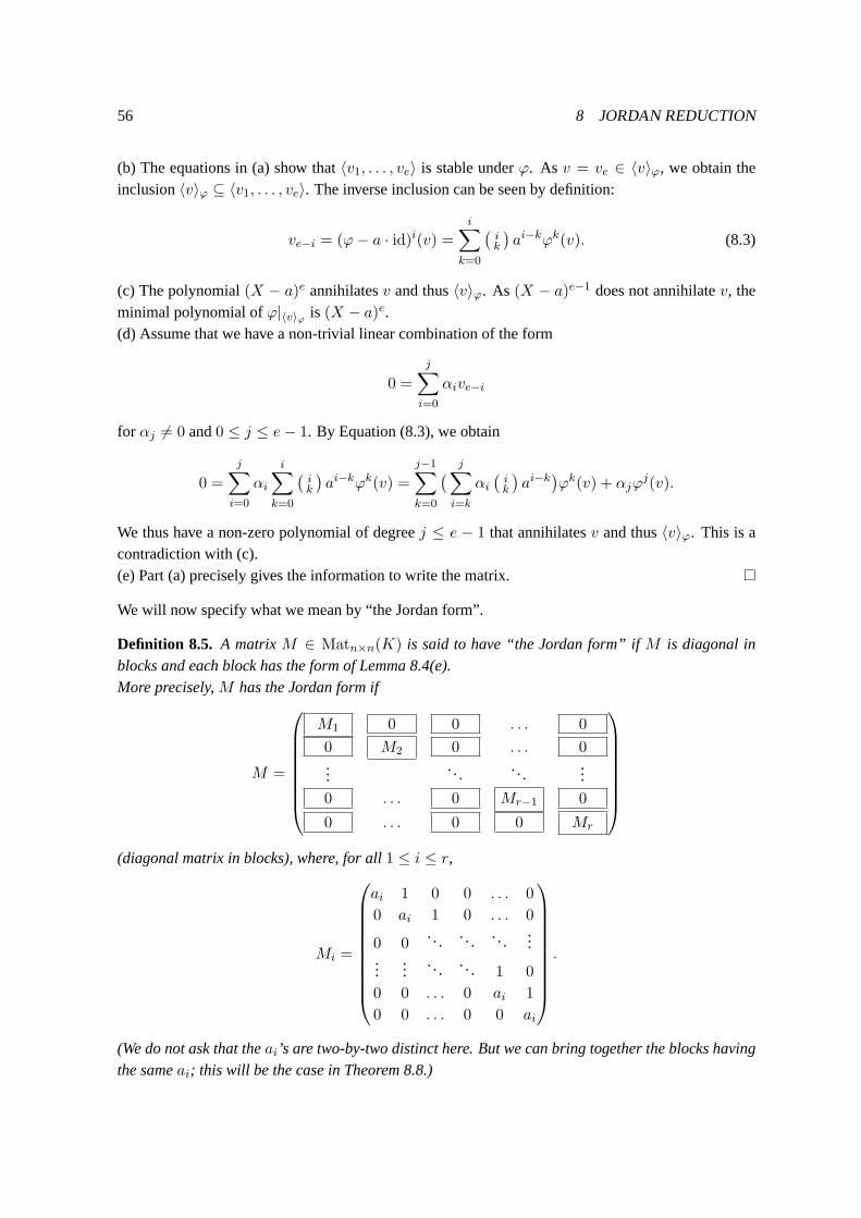
56 8 JORDAN REDUCTION
(b) The equations in (a) show that〈v1, . . . , ve〉 is stable underϕ. As v = ve ∈ 〈v〉ϕ, we obtain theinclusion〈v〉ϕ ⊆ 〈v1, . . . , ve〉. The inverse inclusion can be seen by definition:
ve−i = (ϕ− a · id)i(v) =i∑
k=0
(ik
)ai−kϕk(v). (8.3)
(c) The polynomial(X − a)e annihilatesv and thus〈v〉ϕ. As (X − a)e−1 does not annihilatev, theminimal polynomial ofϕ|〈v〉ϕ is (X − a)e.(d) Assume that we have a non-trivial linear combination of the form
0 =
j∑
i=0
αive−i
for αj 6= 0 and0 ≤ j ≤ e− 1. By Equation (8.3), we obtain
0 =
j∑
i=0
αi
i∑
k=0
(ik
)ai−kϕk(v) =
j−1∑
k=0
( j∑
i=k
αi(ik
)ai−k
)ϕk(v) + αjϕ
j(v).
We thus have a non-zero polynomial of degreej ≤ e − 1 that annihilatesv and thus〈v〉ϕ. This is acontradiction with (c).(e) Part (a) precisely gives the information to write the matrix.
We will now specify what we mean by “the Jordan form”.
Definition 8.5. A matrixM ∈ Matn×n(K) is said to have “the Jordan form” ifM is diagonal inblocks and each block has the form of Lemma 8.4(e).More precisely,M has the Jordan form if
M =
M1 0 0 . . . 0
0 M2 0 . . . 0...
. .. . . ....
0 . . . 0 Mr−1 0
0 . . . 0 0 Mr
(diagonal matrix in blocks), where, for all1 ≤ i ≤ r,
Mi =
ai 1 0 0 . . . 0
0 ai 1 0 . . . 0
0 0. . . . .. .. .
......
.... . . . .. 1 0
0 0 . . . 0 ai 1
0 0 . . . 0 0 ai
.
(We do not ask that theai’s are two-by-two distinct here. But we can bring together the blocks havingthe sameai; this will be the case in Theorem 8.8.)
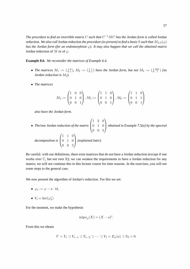
57
The procedure to find an invertible matrixC such thatC−1MC has the Jordan form is calledJordanreduction. We also callJordan reductionthe procedure (to present) to find a basisS such thatMS,S(ϕ)
has the Jordan form (for an endomorphismϕ). It may also happen that we call the obtained matrixJordan reduction ofM or ofϕ.
Example 8.6. We reconsider the matrices of Example 6.4.
• The matricesM1 := ( 1 00 1 ), M2 := ( 1 1
0 1 ) have the Jordan form, but notM3 := ( 1 6910 1 ) (its
Jordan reduction isM2).
• The matrices
M4 :=
1 0 0
0 1 0
0 0 1
,M5 :=
1 1 0
0 1 0
0 0 1
,M6 :=
1 1 0
0 1 1
0 0 1
also have the Jordan form.
• The/one Jordan reduction of the matrix
1 2 0
0 1 0
0 0 5
obtained in Example 7.5(a) by the spectral
decomposition is
1 1 0
0 1 0
0 0 5
(explained later).
Be careful: with our definitions, there exist matrices that do not have a Jordan reduction (except if oneworks overC, but not overR); we can weaken the requirements to have a Jordan reduction for anymatrix; we will not continue this in this lecture course for time reasons. In the exercises, you will seesome steps to the general case.
We now present the algorithm of Jordan’s reduction. For this we set:
• ϕa := ϕ− a · id,
• Vi = ker(ϕia)
For the moment, we make the hypothesis
mipoϕ(X) = (X − a)e.
From this we obtain
V = Ve ⊃ Ve−1 ⊃ Ve−2 ⊃ · · · ⊃ V1 = Eϕ(a) ⊃ V0 = 0.
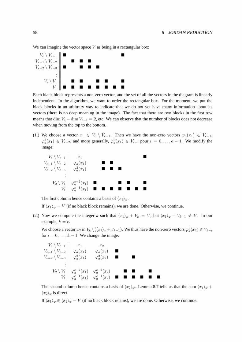
58 8 JORDAN REDUCTION
We can imagine the vector spaceV as being in a rectangular box:
Ve \ Ve−1 � �
Ve−1 \ Ve−2 � � �
Ve−2 \ Ve−3 � � � �
...V2 \ V1 � � � � �
V1 � � � � � � � �
Each black block represents a non-zero vector, and the set of all the vectors in the diagram is linearlyindependent. In the algorithm, we want to order the rectangular box. For the moment, we put theblack blocks in an arbitrary way to indicate that we do not yet have many information about itsvectors (there is no deep meaning in the image). The fact that there are two blocks in the first rowmeans thatdimVe − dimVe−1 = 2, etc. We can observe that the number of blocks does not decreasewhen moving from the top to the bottom.
(1.) We choose a vectorx1 ∈ Ve \ Ve−1. Then we have the non-zero vectorsϕa(x1) ∈ Ve−1,ϕ2a(x1) ∈ Ve−2, and more generally,ϕia(x1) ∈ Ve−i pour i = 0, . . . , e − 1. We modify the
image:
Ve \ Ve−1 x1 �
Ve−1 \ Ve−2 ϕa(x1) � �
Ve−2 \ Ve−3 ϕ2a(x1) � � �
...V2 \ V1 ϕe−2
a (x1) � � � �
V1 ϕe−1a (x1) � � � � � � �
The first column hence contains a basis of〈x1〉ϕ.
If 〈x1〉ϕ = V (if no black block remains), we are done. Otherwise, we continue.
(2.) Now we compute the integerk such that〈x1〉ϕ + Vk = V , but 〈x1〉ϕ + Vk−1 6= V . In ourexample,k = e.
We choose a vectorx2 in Vk \ (〈x1〉ϕ+Vk−1). We thus have the non-zero vectorsϕia(x2) ∈ Vk−ifor i = 0, . . . , k − 1. We change the image:
Ve \ Ve−1 x1 x2Ve−1 \ Ve−2 ϕa(x1) ϕa(x2) �
Ve−2 \ Ve−3 ϕ2a(x1) ϕ2
a(x2) � �
...V2 \ V1 ϕe−2
a (x1) ϕe−2a (x2) � � �
V1 ϕe−1a (x1) ϕe−1
a (x2) � � � � � �
The second column hence contains a basis of〈x2〉ϕ. Lemma 8.7 tells us that the sum〈x1〉ϕ +
〈x2〉ϕ is direct.
If 〈x1〉ϕ ⊕ 〈x2〉ϕ = V (if no black block relains), we are done. Otherwise, we continue.
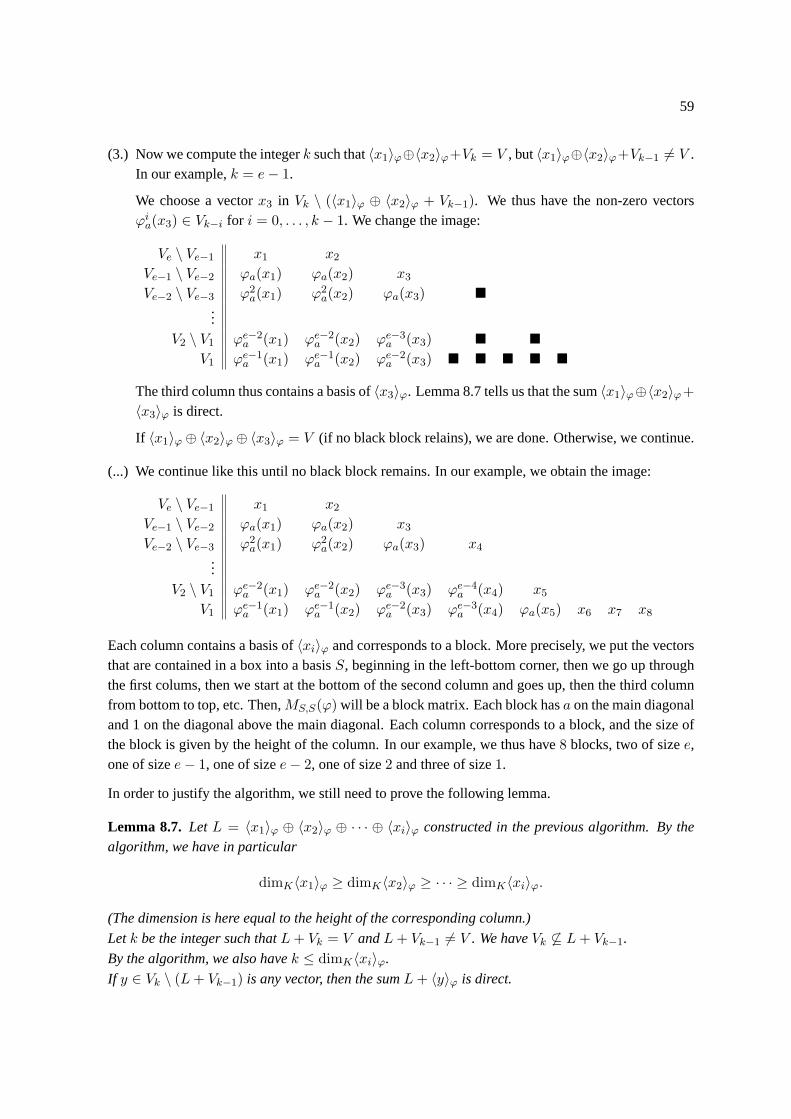
59
(3.) Now we compute the integerk such that〈x1〉ϕ⊕〈x2〉ϕ+Vk = V , but〈x1〉ϕ⊕〈x2〉ϕ+Vk−1 6= V .In our example,k = e− 1.
We choose a vectorx3 in Vk \ (〈x1〉ϕ ⊕ 〈x2〉ϕ + Vk−1). We thus have the non-zero vectorsϕia(x3) ∈ Vk−i for i = 0, . . . , k − 1. We change the image:
Ve \ Ve−1 x1 x2Ve−1 \ Ve−2 ϕa(x1) ϕa(x2) x3Ve−2 \ Ve−3 ϕ2
a(x1) ϕ2a(x2) ϕa(x3) �
...V2 \ V1 ϕe−2
a (x1) ϕe−2a (x2) ϕe−3
a (x3) � �
V1 ϕe−1a (x1) ϕe−1
a (x2) ϕe−2a (x3) � � � � �
The third column thus contains a basis of〈x3〉ϕ. Lemma 8.7 tells us that the sum〈x1〉ϕ⊕〈x2〉ϕ+〈x3〉ϕ is direct.
If 〈x1〉ϕ ⊕ 〈x2〉ϕ ⊕ 〈x3〉ϕ = V (if no black block relains), we are done. Otherwise, we continue.
(...) We continue like this until no black block remains. In our example, we obtain the image:
Ve \ Ve−1 x1 x2Ve−1 \ Ve−2 ϕa(x1) ϕa(x2) x3Ve−2 \ Ve−3 ϕ2
a(x1) ϕ2a(x2) ϕa(x3) x4
...V2 \ V1 ϕe−2
a (x1) ϕe−2a (x2) ϕe−3
a (x3) ϕe−4a (x4) x5
V1 ϕe−1a (x1) ϕe−1
a (x2) ϕe−2a (x3) ϕe−3
a (x4) ϕa(x5) x6 x7 x8
Each column contains a basis of〈xi〉ϕ and corresponds to a block. More precisely, we put the vectorsthat are contained in a box into a basisS, beginning in the left-bottom corner, then we go up throughthe first colums, then we start at the bottom of the second column and goes up, then the third columnfrom bottom to top, etc. Then,MS,S(ϕ) will be a block matrix. Each block hasa on the main diagonaland 1 on the diagonal above the main diagonal. Each column corresponds toa block, and the size ofthe block is given by the height of the column. In our example, we thus have8 blocks, two of sizee,one of sizee− 1, one of sizee− 2, one of size2 and three of size1.
In order to justify the algorithm, we still need to prove the following lemma.
Lemma 8.7. Let L = 〈x1〉ϕ ⊕ 〈x2〉ϕ ⊕ · · · ⊕ 〈xi〉ϕ constructed in the previous algorithm. By thealgorithm, we have in particular
dimK〈x1〉ϕ ≥ dimK〈x2〉ϕ ≥ · · · ≥ dimK〈xi〉ϕ.
(The dimension is here equal to the height of the corresponding column.)
Letk be the integer such thatL+ Vk = V andL+ Vk−1 6= V . We haveVk 6⊆ L+ Vk−1.
By the algorithm, we also havek ≤ dimK〈xi〉ϕ.
If y ∈ Vk \ (L+ Vk−1) is any vector, then the sumL+ 〈y〉ϕ is direct.
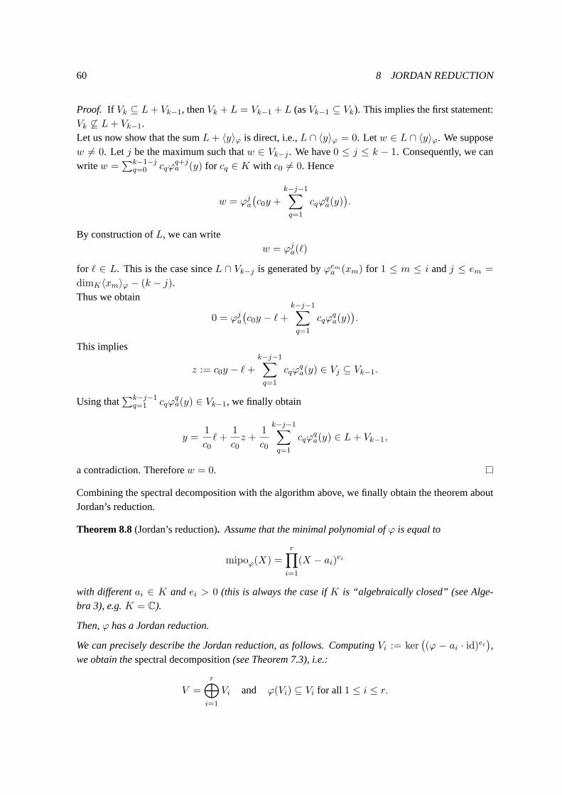
60 8 JORDAN REDUCTION
Proof. If Vk ⊆ L+ Vk−1, thenVk + L = Vk−1 + L (asVk−1 ⊆ Vk). This implies the first statement:Vk 6⊆ L+ Vk−1.Let us now show that the sumL+ 〈y〉ϕ is direct, i.e.,L ∩ 〈y〉ϕ = 0. Letw ∈ L ∩ 〈y〉ϕ. We supposew 6= 0. Let j be the maximum such thatw ∈ Vk−j . We have0 ≤ j ≤ k − 1. Consequently, we canwritew =
∑k−1−jq=0 cqϕ
q+ja (y) for cq ∈ K with c0 6= 0. Hence
w = ϕja(c0y +
k−j−1∑
q=1
cqϕqa(y)
).
By construction ofL, we can writew = ϕja(ℓ)
for ℓ ∈ L. This is the case sinceL ∩ Vk−j is generated byϕema (xm) for 1 ≤ m ≤ i andj ≤ em =
dimK〈xm〉ϕ − (k − j).Thus we obtain
0 = ϕja(c0y − ℓ+
k−j−1∑
q=1
cqϕqa(y)
).
This implies
z := c0y − ℓ+
k−j−1∑
q=1
cqϕqa(y) ∈ Vj ⊆ Vk−1.
Using that∑k−j−1
q=1 cqϕqa(y) ∈ Vk−1, we finally obtain
y =1
c0ℓ+
1
c0z +
1
c0
k−j−1∑
q=1
cqϕqa(y) ∈ L+ Vk−1,
a contradiction. Thereforew = 0.
Combining the spectral decomposition with the algorithm above, we finally obtain the theorem aboutJordan’s reduction.
Theorem 8.8(Jordan’s reduction). Assume that the minimal polynomial ofϕ is equal to
mipoϕ(X) =r∏
i=1
(X − ai)ei
with differentai ∈ K andei > 0 (this is always the case ifK is “algebraically closed” (see Alge-bra 3), e.g.K = C).
Then,ϕ has a Jordan reduction.
We can precisely describe the Jordan reduction, as follows. ComputingVi := ker((ϕ − ai · id)ei
),
we obtain thespectral decomposition(see Theorem 7.3), i.e.:
V =r⊕
i=1
Vi and ϕ(Vi) ⊆ Vi for all 1 ≤ i ≤ r.
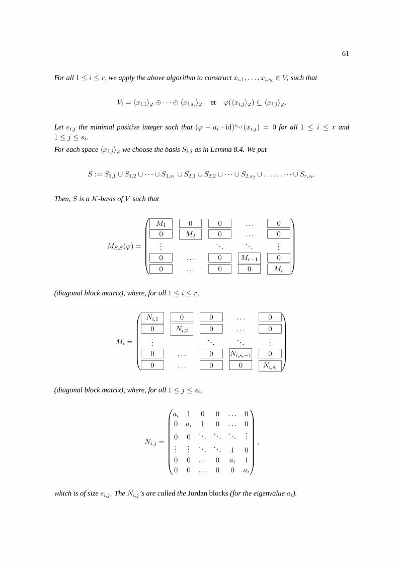
61
For all 1 ≤ i ≤ r, we apply the above algorithm to constructxi,1, . . . , xi,si ∈ Vi such that
Vi = 〈xi,1〉ϕ ⊕ · · · ⊕ 〈xi,si〉ϕ et ϕ(〈xi,j〉ϕ) ⊆ 〈xi,j〉ϕ.
Let ei,j the minimal positive integer such that(ϕ − ai · id)ei,j (xi,j) = 0 for all 1 ≤ i ≤ r and1 ≤ j ≤ si.
For each space〈xi,j〉ϕ we choose the basisSi,j as in Lemma 8.4. We put
S := S1,1 ∪ S1,2 ∪ · · · ∪ S1,s1 ∪ S2,1 ∪ S2,2 ∪ · · · ∪ S2,s2 ∪ . . . . . . · · · ∪ Sr,sr .
Then,S is aK-basis ofV such that
MS,S(ϕ) =
M1 0 0 . . . 0
0 M2 0 . . . 0...
.. . . . ....
0 . . . 0 Mr−1 0
0 . . . 0 0 Mr
(diagonal block matrix), where, for all1 ≤ i ≤ r,
Mi =
Ni,1 0 0 . . . 0
0 Ni,2 0 . . . 0
..... . . . .
...
0 . . . 0 Ni,si−1 0
0 . . . 0 0 Ni,si
(diagonal block matrix), where, for all1 ≤ j ≤ si,
Ni,j =
ai 1 0 0 . . . 0
0 ai 1 0 . . . 0
0 0. .. . . . . ..
......
.... .. . . . 1 0
0 0 . . . 0 ai 1
0 0 . . . 0 0 ai
,
which is of sizeei,j . TheNi,j ’s are called theJordan blocks(for the eigenvalueai).
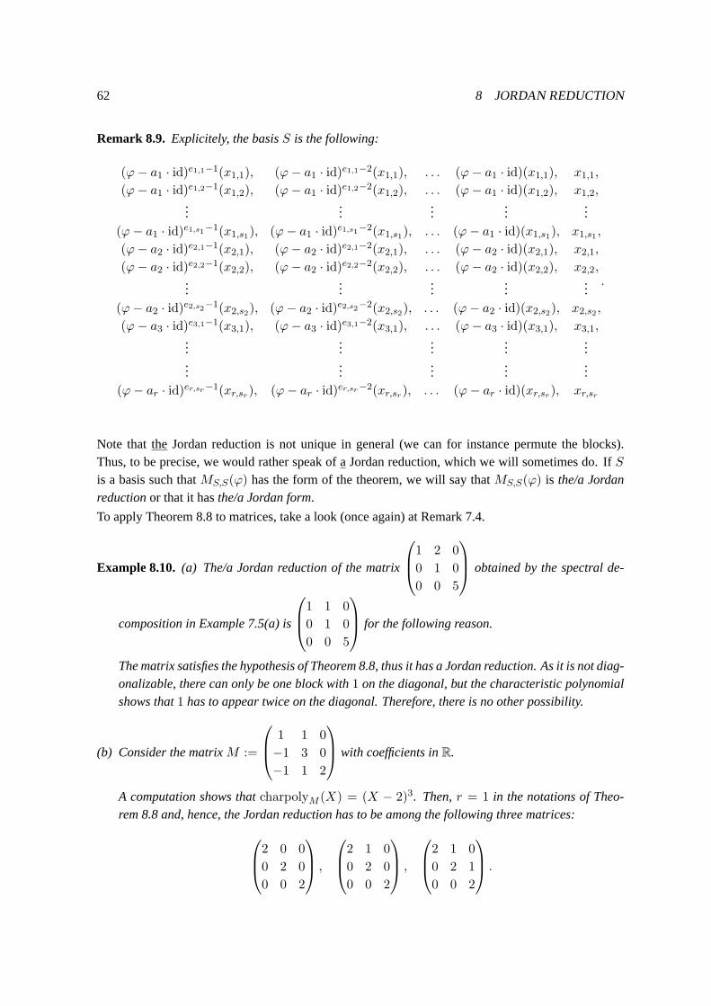
62 8 JORDAN REDUCTION
Remark 8.9. Explicitely, the basisS is the following:
(ϕ− a1 · id)e1,1−1(x1,1), (ϕ− a1 · id)e1,1−2(x1,1), . . . (ϕ− a1 · id)(x1,1), x1,1,
(ϕ− a1 · id)e1,2−1(x1,2), (ϕ− a1 · id)e1,2−2(x1,2), . . . (ϕ− a1 · id)(x1,2), x1,2,...
......
......
(ϕ− a1 · id)e1,s1−1(x1,s1), (ϕ− a1 · id)e1,s1−2(x1,s1), . . . (ϕ− a1 · id)(x1,s1), x1,s1 ,
(ϕ− a2 · id)e2,1−1(x2,1), (ϕ− a2 · id)e2,1−2(x2,1), . . . (ϕ− a2 · id)(x2,1), x2,1,
(ϕ− a2 · id)e2,2−1(x2,2), (ϕ− a2 · id)e2,2−2(x2,2), . . . (ϕ− a2 · id)(x2,2), x2,2,...
......
......
(ϕ− a2 · id)e2,s2−1(x2,s2), (ϕ− a2 · id)e2,s2−2(x2,s2), . . . (ϕ− a2 · id)(x2,s2), x2,s2 ,
(ϕ− a3 · id)e3,1−1(x3,1), (ϕ− a3 · id)e3,1−2(x3,1), . . . (ϕ− a3 · id)(x3,1), x3,1,...
......
......
......
......
...(ϕ− ar · id)er,sr−1(xr,sr), (ϕ− ar · id)er,sr−2(xr,sr), . . . (ϕ− ar · id)(xr,sr), xr,sr
.
Note that theJordan reduction is not unique in general (we can for instance permute the blocks).Thus, to be precise, we would rather speak of aJordan reduction, which we will sometimes do. IfSis a basis such thatMS,S(ϕ) has the form of the theorem, we will say thatMS,S(ϕ) is the/a Jordanreductionor that it hasthe/a Jordan form.
To apply Theorem 8.8 to matrices, take a look (once again) at Remark 7.4.
Example 8.10. (a) The/a Jordan reduction of the matrix
1 2 0
0 1 0
0 0 5
obtained by the spectral de-
composition in Example 7.5(a) is
1 1 0
0 1 0
0 0 5
for the following reason.
The matrix satisfies the hypothesis of Theorem 8.8, thus it has a Jordan reduction. As it is not diag-onalizable, there can only be one block with1 on the diagonal, but the characteristic polynomialshows that1 has to appear twice on the diagonal. Therefore, there is no other possibility.
(b) Consider the matrixM :=
1 1 0
−1 3 0
−1 1 2
with coefficients inR.
A computation shows thatcharpolyM (X) = (X − 2)3. Then,r = 1 in the notations of Theo-rem 8.8 and, hence, the Jordan reduction has to be among the following three matrices:
2 0 0
0 2 0
0 0 2
,
2 1 0
0 2 0
0 0 2
,
2 1 0
0 2 1
0 0 2
.
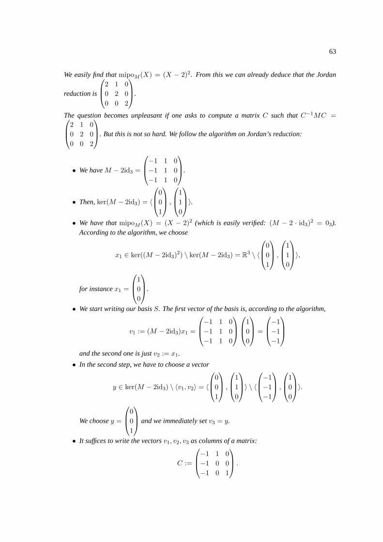
63
We easily find thatmipoM (X) = (X − 2)2. From this we can already deduce that the Jordan
reduction is
2 1 0
0 2 0
0 0 2
.
The question becomes unpleasant if one asks to compute a matrixC such thatC−1MC =2 1 0
0 2 0
0 0 2
. But this is not so hard. We follow the algorithm on Jordan’s reduction:
• We haveM − 2id3 =
−1 1 0
−1 1 0
−1 1 0
.
• Then,ker(M − 2id3) = 〈
0
0
1
,
1
1
0
〉.
• We have thatmipoM (X) = (X − 2)2 (which is easily verified:(M − 2 · id3)2 = 03).According to the algorithm, we choose
x1 ∈ ker((M − 2id3)2) \ ker(M − 2id3) = R3 \ 〈
0
0
1
,
1
1
0
〉,
for instancex1 =
1
0
0
.
• We start writing our basisS. The first vector of the basis is, according to the algorithm,
v1 := (M − 2id3)x1 =
−1 1 0
−1 1 0
−1 1 0
1
0
0
=
−1
−1
−1
and the second one is justv2 := x1.
• In the second step, we have to choose a vector
y ∈ ker(M − 2id3) \ 〈v1, v2〉 = 〈
0
0
1
,
1
1
0
〉 \ 〈
−1
−1
−1
,
1
0
0
〉.
We choosey =
0
0
1
and we immediately setv3 = y.
• It suffices to write the vectorsv1, v2, v3 as columns of a matrix:
C :=
−1 1 0
−1 0 0
−1 0 1
.
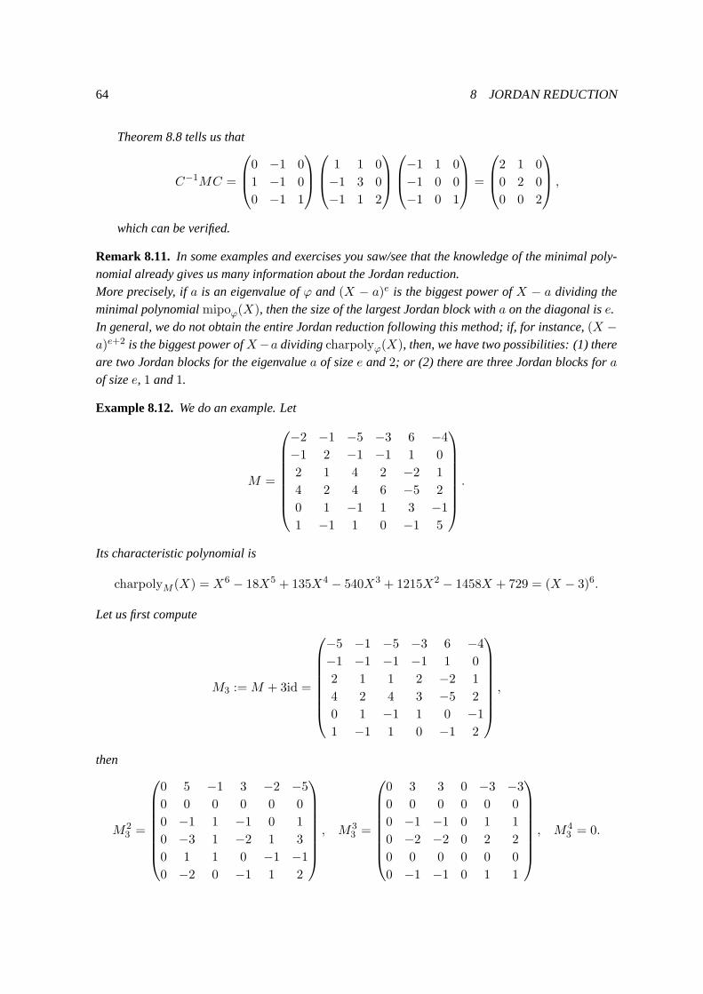
64 8 JORDAN REDUCTION
Theorem 8.8 tells us that
C−1MC =
0 −1 0
1 −1 0
0 −1 1
1 1 0
−1 3 0
−1 1 2
−1 1 0
−1 0 0
−1 0 1
=
2 1 0
0 2 0
0 0 2
,
which can be verified.
Remark 8.11. In some examples and exercises you saw/see that the knowledge of the minimal poly-nomial already gives us many information about the Jordan reduction.More precisely, ifa is an eigenvalue ofϕ and (X − a)e is the biggest power ofX − a dividing theminimal polynomialmipoϕ(X), then the size of the largest Jordan block witha on the diagonal ise.In general, we do not obtain the entire Jordan reduction following this method; if, for instance,(X −a)e+2 is the biggest power ofX−a dividingcharpolyϕ(X), then, we have two possibilities: (1) thereare two Jordan blocks for the eigenvaluea of sizee and2; or (2) there are three Jordan blocks foraof sizee, 1 and1.
Example 8.12.We do an example. Let
M =
−2 −1 −5 −3 6 −4
−1 2 −1 −1 1 0
2 1 4 2 −2 1
4 2 4 6 −5 2
0 1 −1 1 3 −1
1 −1 1 0 −1 5
.
Its characteristic polynomial is
charpolyM (X) = X6 − 18X5 + 135X4 − 540X3 + 1215X2 − 1458X + 729 = (X − 3)6.
Let us first compute
M3 :=M + 3id =
−5 −1 −5 −3 6 −4
−1 −1 −1 −1 1 0
2 1 1 2 −2 1
4 2 4 3 −5 2
0 1 −1 1 0 −1
1 −1 1 0 −1 2
,
then
M23 =
0 5 −1 3 −2 −5
0 0 0 0 0 0
0 −1 1 −1 0 1
0 −3 1 −2 1 3
0 1 1 0 −1 −1
0 −2 0 −1 1 2
, M33 =
0 3 3 0 −3 −3
0 0 0 0 0 0
0 −1 −1 0 1 1
0 −2 −2 0 2 2
0 0 0 0 0 0
0 −1 −1 0 1 1
, M43 = 0.

65
We thus have
mipoM (X) = (X − 3)4
and
V4 = ker(M43 ) = R6 ) V3 ) V2 ) V1 = EM (3) ) 0.
We first compute
V3 = ker(M33 ) = ker
0 1 1 0 −1 −1
0 0 0 0 0 0
0 0 0 0 0 0
0 0 0 0 0 0
0 0 0 0 0 0
0 0 0 0 0 0
= 〈
1
0
0
0
0
0
,
0
0
0
1
0
0
,
0
1
−1
0
0
0
,
0
0
0
0
1
−1
,
0
1
0
0
1
0
〉.
In fact, it is not necessary for the algorithm to give an entire basis ofV3, it suffices to find a vector
that does not belong to the kernel. It is very easy. We will takex1 =
010000
and we compute
x1 =
010000
,M3x1 =
−1−1121−1
,M2
3x1 =
50−1−31−2
,M3
3x1 =
30−1−20−1
.
We thus already have a Jordan block of size4. Thus there is either a block of size2, or two blocks ofsize1. We now compute
V2 = ker(M2
3) = ker
0 1 1 0 −1 −1
0 0 −6 3 3 0
0 0 2 −1 −1 0
0 0 4 −2 −2 0
0 0 2 −1 −1 0
0 0 0 0 0 0
= ker
0 1 1 0 −1 −1
0 0 1 −1/2 −1/2 0
0 0 0 0 0 0
0 0 0 0 0 0
0 0 0 0 0 0
0 0 0 0 0 0
= ker
0 1 0 1/2 −1/2 −1
0 0 1 −1/2 −1/2 0
0 0 0 0 0 0
0 0 0 0 0 0
0 0 0 0 0 0
0 0 0 0 0 0
= 〈
1
0
0
0
0
0
,
0
1
0
0
0
1
,
0
1/2
1/2
0
1
0
,
0
−1/2
1/2
1
0
0
〉.

66 8 JORDAN REDUCTION
Finally, we compute the eigenspace for the eigenvalue3:
V1 = ker(M3) = ker
−5 −1 −5 −3 6 −4
−1 −1 −1 −1 1 0
2 1 1 2 −2 1
4 2 4 3 −5 2
0 1 −1 1 0 −1
1 −1 1 0 −1 2
= ker
1 −1 1 0 −1 2
0 1 −1 1 0 −1
0 −6 0 −3 1 6
0 −2 0 −1 0 2
0 3 −1 2 0 −3
0 6 0 3 −1 −6
= ker
1 0 0 1 −1 1
0 1 −1 1 0 −1
0 0 −6 3 1 0
0 0 −2 1 0 0
0 0 2 −1 0 0
0 0 6 −3 −1 0
= ker
1 0 0 1 −1 1
0 1 −1 1 0 −1
0 0 1 −1/2 0 0
0 0 −6 3 1 0
0 0 2 −1 0 0
0 0 0 0 0 0
= ker
1 0 0 1 −1 1
0 1 0 1/2 0 −1
0 0 1 −1/2 0 0
0 0 0 0 1 0
0 0 0 0 0 0
0 0 0 0 0 0
= ker
1 0 0 1 0 1
0 1 0 1/2 0 −1
0 0 1 −1/2 0 0
0 0 0 0 1 0
0 0 0 0 0 0
0 0 0 0 0 0
= 〈
−1
1
0
0
0
1
,
−1
−1/2
1/2
1
0
0
〉.
Thus there are2 eigenvectors, hence two blocks in total. Thus the second block is of size2. We haveto find a vector inV2 which is not inV1 + 〈x1,M3x1,M
23x1,M
33x1〉, thus an element of
〈
1
0
0
0
0
0
,
0
1
0
0
0
1
,
0
1/2
1/2
0
1
0
,
0
−1/2
1/2
1
0
0
〉 \ 〈
−1
1
0
0
0
1
,
−1
−1/2
1/2
1
0
0
,
0
1
0
0
0
0
,
−1
−1
1
2
1
−1
,
5
0
−1
−3
1
−2
,
3
0
−1
−2
0
−1
〉.
To find such an element, we test if the vectors (one by one) of the basis ofV2 are linearly independent
form the space on the right. We are lucky that it already works out forx2 :=
100000
(as one can see
from a standard computation). We thus calculate
x2 =
1
0
0
0
0
0
, M3x2 =
−5
−1
2
4
0
1
.
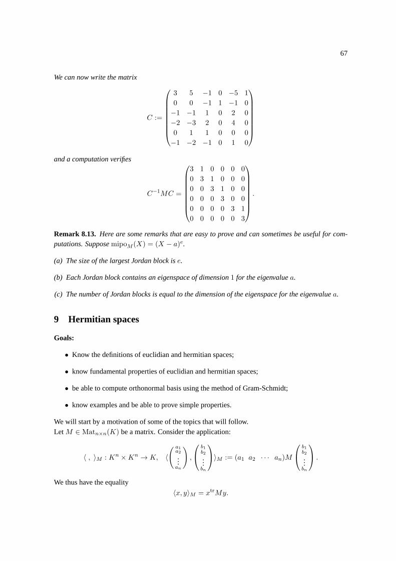
67
We can now write the matrix
C :=
3 5 −1 0 −5 1
0 0 −1 1 −1 0
−1 −1 1 0 2 0
−2 −3 2 0 4 0
0 1 1 0 0 0
−1 −2 −1 0 1 0
and a computation verifies
C−1MC =
3 1 0 0 0 0
0 3 1 0 0 0
0 0 3 1 0 0
0 0 0 3 0 0
0 0 0 0 3 1
0 0 0 0 0 3
.
Remark 8.13. Here are some remarks that are easy to prove and can sometimes be useful for com-putations. SupposemipoM (X) = (X − a)e.
(a) The size of the largest Jordan block ise.
(b) Each Jordan block contains an eigenspace of dimension1 for the eigenvaluea.
(c) The number of Jordan blocks is equal to the dimension of the eigenspace for the eigenvaluea.
9 Hermitian spaces
Goals:
• Know the definitions of euclidian and hermitian spaces;
• know fundamental properties of euclidian and hermitian spaces;
• be able to compute orthonormal basis using the method of Gram-Schmidt;
• know examples and be able to prove simple properties.
We will start by a motivation of some of the topics that will follow.
LetM ∈ Matn×n(K) be a matrix. Consider the application:
〈 , 〉M : Kn ×Kn → K, 〈( a1a2...an
),
b1b2...bn
〉M := (a1 a2 · · · an)M
b1b2...bn
.
We thus have the equality
〈x, y〉M = xtrMy.
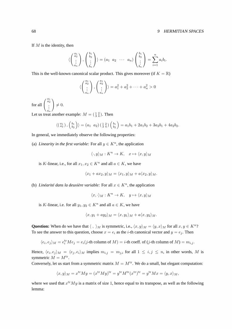
68 9 HERMITIAN SPACES
If M is the identity, then
〈( a1a2...an
),
b1b2...bn
〉 = (a1 a2 · · · an)
b1b2...bn
=
n∑
i=1
aibi.
This is the well-known canonical scalar product. This gives moreover (ifK = R)
〈( a1a2...an
),
( a1a2...an
)〉 = a21 + a22 + · · ·+ a2n > 0
for all
( a1a2...an
)6= 0.
Let us treat another example:M = ( 1 23 4 ). Then
〈( a1a2 ) ,(b1b2
)〉 = (a1 a2) ( 1 2
3 4 )(b1b2
)= a1b1 + 2a1b2 + 3a2b1 + 4a2b2.
In general, we immediately observe the following properties:
(a) Linearity in the first variable:For ally ∈ Kn, the application
〈·, y〉M : Kn → K, x 7→ 〈x, y〉M
isK-linear, i.e., for allx1, x2 ∈ Kn and alla ∈ K, we have
〈x1 + ax2, y〉M = 〈x1, y〉M + a〈x2, y〉M .
(b) Linéarité dans la deuxière variable:For allx ∈ Kn, the application
〈x, ·〉M : Kn → K, y 7→ 〈x, y〉M
isK-linear, i.e. for ally1, y2 ∈ Kn and alla ∈ K, we have
〈x, y1 + ay2〉M = 〈x, y1〉M + a〈x, y2〉M .
Question: When do we have that〈 , 〉M is symmetric, i.e.,〈x, y〉M = 〈y, x〉M for all x, y ∈ Kn?To see the answer to this question, choosex = ei as thei-th canonical vector andy = ej . Then
〈ei, ej〉M = etri Mej = ei(j-th column ofM) = i-th coeff. of (j-th column ofM ) = mi,j .
Hence,〈ei, ej〉M = 〈ej , ei〉M impliesmi,j = mj,i for all 1 ≤ i, j ≤ n, in other words,M issymmetricM =M tr.Conversely, let us start from a symmetric matrixM =M tr. We do a small, but elegant computation:
〈x, y〉M = xtrMy = (xtrMy)tr = ytrM tr(xtr)tr = ytrMx = 〈y, x〉M ,
where we used thatxtrMy is a matrix of size1, hence equal to its transpose, as well as the followinglemma:
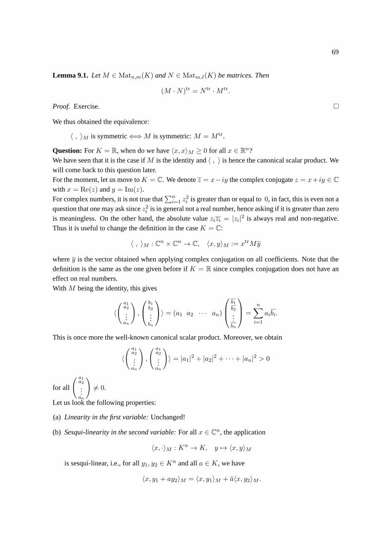
69
Lemma 9.1. LetM ∈ Matn,m(K) andN ∈ Matm,ℓ(K) be matrices. Then
(M ·N)tr = N tr ·M tr.
Proof. Exercise.
We thus obtained the equivalence:
〈 , 〉M is symmetric⇐⇒M is symmetric:M =M tr.
Question: ForK = R, when do we have〈x, x〉M ≥ 0 for all x ∈ Rn?We have seen that it is the case ifM is the identity and〈 , 〉 is hence the canonical scalar product. Wewill come back to this question later.For the moment, let us move toK = C. We denotez = x− iy the complex conjugatez = x+ iy ∈ Cwith x = Re(z) andy = Im(z).For complex numbers, it is not true that
∑ni=1 z
2i is greater than or equal to0, in fact, this is even not a
question that one may ask sincez2i is in general not a real number, hence asking if it is greater than zerois meaningless. On the other hand, the absolute valuezizi = |zi|2 is always real and non-negative.Thus it is useful to change the definition in the caseK = C:
〈 , 〉M : Cn × Cn → C, 〈x, y〉M := xtrMy
wherey is the vector obtained when applying complex conjugation on all coefficients.Note that thedefinition is the same as the one given before ifK = R since complex conjugation does not have aneffect on real numbers.With M being the identity, this gives
〈( a1a2...an
),
b1b2...bn
〉 = (a1 a2 · · · an)
b1b2...bn
=
n∑
i=1
aibi.
This is once more the well-known canonical scalar product. Moreover, we obtain
〈( a1a2...an
),
( a1a2...an
)〉 = |a1|2 + |a2|2 + · · ·+ |an|2 > 0
for all
( a1a2...an
)6= 0.
Let us look the following properties:
(a) Linearity in the first variable:Unchanged!
(b) Sesqui-linearity in the second variable:For allx ∈ Cn, the application
〈x, ·〉M : Kn → K, y 7→ 〈x, y〉M
is sesqui-linear, i.e., for ally1, y2 ∈ Kn and alla ∈ K, we have
〈x, y1 + ay2〉M = 〈x, y1〉M + a〈x, y2〉M .
70 9 HERMITIAN SPACES
By the same computations as above, we obtain the equivalence:
〈x, y〉M = 〈y, x〉M for all x, y ∈ Cn ⇐⇒M =M tr.
A matrixM such thatM =M tr is calledhermitian.For the sequel of this section we setK = R or K = C.
Definition 9.2. LetV be aK-vector space. An application
〈·, ·〉 : V × V → K, (v, w) 7→ 〈v, w〉
is calledherlitian formif for all v, v1, v2, w, w1, w2 ∈ V and for alla, b ∈ K we have
• 〈av1 + v2, w〉 = a〈v1, w〉+ 〈v2, w〉 (linearity in the first variable),
• 〈v, bw1 + w2〉 = b〈v, w1〉+ 〈v, w2〉 (sesqui-linearityin the second variable) and
• 〈v, w〉 = 〈w, v〉.
A hermitian form〈·, ·〉 is said to bepositiveif
• ∀ v ∈ V : 〈v, v〉 ≥ 0. (Note that〈v, v〉 = 〈v, v〉, whence〈v, v〉 ∈ R.)
It is said to bepositive definiteif
• ∀ 0 6= v ∈ V : 〈v, v〉 > 0.
A hermitian positive definite form is also called ascalar product.We callhermitian spaceany tuple(V, 〈·, ·〉) where〈·, ·〉 is a positive definite hermitian form.
Remark 9.3. Note that forK = R the last two conditions of the definition of a hermitian form read
• 〈v, bw1 + w2〉 = b〈v, w1〉+ 〈v, w2〉 (linearity in the second variable) and
• ∀ v ∈ V ∀w ∈W : 〈v, w〉 = 〈w, v〉.
We refer this to as a bilinearsymmetricform.In the literature, ifK = R, one rather uses the nameeuclidian spacein stead of hermitian space(which is often reserved forK = C). Here, to simplify the terminology, we will always speak ofhermitian spaces, even ifK = R.
We have already seen the canonical scalar products forRn andCn. Similar definitions can also bemade in spaces of functions (of finite dimension):
Example 9.4. (a) The canonical scalar product〈 , 〉M for M the identity is indeed a scalar productif K = R or K = C.
(b) LetC = {f : [0, 1] → R | f is continuoud} be the set of all continuous functions from[0, 1] toR.It is anR-vector space for+ and· defined pointwise. The application
〈·, ·〉 : C × C → R, 〈f, g〉 =∫ 1
0f(x)g(x)dx
is a hermitian positive definite form.

71
(c) LetC = {f : [0, 1] → C | f is continuous} be the set of all continuous functions from[0, 1] toC.It is a C-vector space for+ and· defined pointwise. The application
〈·, ·〉 : C × C → C, 〈f, g〉 =∫ 1
0f(x)g(x)dx
is a hermitian positive definite form.
Definition 9.5. Let (V, 〈·, ·〉) be a hermitianK-space.
We say thatv, w ∈ V areorthogonalv ⊥ w if 〈v, w〉 = 0. Note:v ⊥ w ⇔ w ⊥ v.
LetW ≤ V be a subspace. We say thatv ∈ V andW areorthogonalv ⊥W if v ⊥ w for all w ∈W .Note:v ⊥W ⇔W ⊥ v (with evident defintions).
Let U ≤ V be another subspace. We say thatU andW are orthogonalU ⊥ W if U ⊥ w for allw ∈W . Note:U ⊥W ⇔W ⊥ U .
Theorthogonal complement ofW is defined as
W⊥ = {v ∈ V | v ⊥W}.
Thenorm (“length”) of v ∈ V is defined as|v| :=√〈v, v〉 and |v − w| is said to be thedistance
betweenv andw.
Proposition 9.6. Let (V, 〈·, ·〉) be a hermitianK-space.
(a) For all v ∈ V we have|v| ≥ 0 and|v| = 0 ⇔ v = 0.
(b) For all v ∈ V and alla ∈ K we have:|a · v|︸ ︷︷ ︸|·| in V
= |a|︸︷︷︸|·| in K
· |v|︸︷︷︸|·| in V
.
(c) For all v, w ∈ V we have|〈v, w〉|︸ ︷︷ ︸|·| in K
≤ |v|︸︷︷︸|·| in V
· |w|︸︷︷︸|·| in V
(Cauchy-Schwarz inequality).
(d) For all v, w ∈ V we have|v + w|︸ ︷︷ ︸|·| in V
≤ |v|︸︷︷︸|·| in V
+ |w|︸︷︷︸|·| in V
(triangular inequality).
Proof. (a) Defintion.
(b) |a · v|2 = 〈a · v, a · v〉 = a · a · 〈v, v〉 = |a|2 · |v|2.(c) 1st case:w = 0. Then,〈v, w〉 = 〈v, 0 · w〉 = 0〈v, w〉 = 0, whence|〈v, w〉| = 0 = |v| · |w|.2nd case:w 6= 0. Let c := 〈v,w〉
|w|2 . Then
0 ≤ |w|2 · 〈v − c · w, v − c · w〉= |w|2 · 〈v, v〉 − |w|2 · c · 〈w, v〉 − |w|2 · c · 〈v, w〉+ |w|2 · c · c · 〈w,w〉= |w|2 · |v|2 − 〈v, w〉 · 〈w, v〉︸ ︷︷ ︸
=|〈v,w〉|
−〈v, w〉 · 〈v, w〉+ 〈v, w〉 · 〈v, w〉︸ ︷︷ ︸=0
.
72 9 HERMITIAN SPACES
(d)
|v + w|2 = 〈v + w, v + w〉= 〈v, v〉+ 〈v, w〉+ 〈w, v〉+ 〈w,w〉= |v|2 + |w|2 + 〈v, w〉+ 〈v, w〉= |v|2 + |w|2 + 2 · Re(〈v, w〉)≤ |v|2 + |w|2 + 2 · |〈v, w〉|≤ |v|2 + |w|2 + 2 · |v| · |w|= (|v|+ |w|)2.
Proposition 9.7(Pythagoras). If v ⊥ w, then|v + w|2 = |v|2 + |w|2.
Proof. |v + w|2 = 〈v + w, v + w〉 = 〈v, v〉+ 〈w,w〉 = |v|2 + |w|2.
Note that any hermitian positive definite form is non-degenerate: if〈v, w〉 = 0 for all w ∈W , then inparticular〈v, v〉 = |v|2 = 0, whencev = 0. The same argument also shows thatw = 0 si 〈v, w〉 = 0
for all v ∈ V .
Definition 9.8. Let (V, 〈·, ·〉) be a hermitianK-space andS = {si | i ∈ I} (with I a set, e.g.,S = {s1, . . . , sn} if I = {1, 2, . . . , n}).We say thatS is anorthogonal systemif
• 〈si, si〉 > 0 for all i ∈ I and
• 〈si, sj〉 = 0 for all i, j ∈ I, i 6= j.
We say thatS is anorthonormal systemif 〈si, sj〉 = δi,j pour touti, j ∈ I.If S is a basis ofV which is an orthogonal/orthonormal system, we speak of anorthogonal/ortho-normal basis.
Example 9.9. The canonical basis ofRn (or ofCn) is an orthonormal basis for the canonical scalarproduct of Example 9.4.
Proposition 9.10 (Gram-Schmidt Orthonormalization). Let (V, 〈·, ·〉) be a hermitianK-space ands1, s2, . . . , sn ∈ V K-linearly independent vectors.Themethod of Gram-Schmidt(see proof) computes the vectorst1, t2, . . . , tn ∈ V such that
• 〈ti, tj〉 = δi,j for all 1 ≤ i, j ≤ n and
• 〈s1, s2, . . . , sr〉 = 〈t1, t2, . . . , tr〉 for all 1 ≤ r ≤ n (in words: the subspaces ofV generatedbys1, s2, . . . , sr and byt1, t2, . . . , tr are equal for all1 ≤ r ≤ n).
Proof. We present the method of Gram-Schmidt.It is an induction onr = 1, 2, . . . , n; hence there aren steps.r = 1. t1 :=
s1|s1| .
73
r ⇒ r + 1. By induction hypothesis we already havet1, . . . , tr such that〈ti, tj〉 = δi,j for all 1 ≤i, j ≤ r and〈s1, s2, . . . , sr〉 = 〈t1, t2, . . . , tr〉.We have to findtr+1. First we define
wr+1 := sr+1 −r∑
i=1
〈sr+1, ti〉ti.
This vector satisfies for all1 ≤ j ≤ r
〈wr+1, tj〉 = 〈sr+1 −r∑
i=1
〈sr+1, ti〉ti, tj〉
= 〈sr+1, tj〉 −r∑
i=1
〈〈sr+1, ti〉ti, tj〉
= 〈sr+1, tj〉 − 〈〈sr+1, tj〉tj , tj〉= 〈sr+1, tj〉 − 〈sr+1, tj〉 · 〈tj , tj〉= 0
Since〈s1, s2, . . . , sr〉 = 〈t1, t2, . . . , tr〉, we havewr+1 6∈ 〈t1, t2, . . . , tr〉, hence, in particular,wr+1 6=0. This allows us to define
tr+1 :=wr+1
|wr+1|.
This vector clearly satisfies〈tr+1, ti〉 = δr+1,i for all 1 ≤ i ≤ r + 1 and〈s1, s2, . . . , sr, sr+1〉 =
〈t1, t2, . . . , tr, tr+1〉.
Example 9.11.We apply the method of Gram-Schmidt to the following vectors:
s1 =
110101
, s2 =
13−23−25
, s3 =
−152−3−63
surR6 avec le produit scalaire canonique.
(1) Let us compute the length ofs1:
|s1| =√4 = 2.
Thus
t1 =1
2s1 =
1/21/20
1/20
1/2
.
(2) Let us now compute
〈s2, t1〉 = 〈
13−23−25
,
1/21/20
1/20
1/2
〉 = 6.
74 9 HERMITIAN SPACES
Thus
w2 := s2 − 〈s2, t1〉t1 =
13−23−25
− 6
1/21/20
1/20
1/2
=
−20−20−22
.
The length ofw2 is|w2| =
√16 = 4.
Donc
t2 =1
4w2 =
−1/20
−1/20
−1/21/2
.
(3) Now compute
〈s3, t1〉 = 〈
−152−3−63
,
1/21/20
1/20
1/2
〉 = 2
and
〈s3, t2〉 = 〈
−152−3−63
,
−1/20
−1/20
−1/21/2
〉 = 4.
Thus
w3 := s3 − 〈s3, t1〉t1 − 〈s3, t2〉t2 =
−152−3−63
− 2
1/21/20
1/20
1/2
− 4
−1/20
−1/20
−1/21/2
=
044−4−40
.
The length ofw3 is|w3| =
√64 = 8.
Thus
t3 =1
8w3 =
01/21/2−1/2−1/20
.
Corollary 9.12. Let (V, 〈·, ·〉) be a hermitianK-space of finite dimension (or even countable). Then,V has an orthonormalK-basis.
Proof. Direct consequence of Gram-Schmidt 9.10.
Corollary 9.13. Let(V, 〈·, ·〉) be a hermitianK-space andW ≤ V be a subspace of finite dimension.Let s1, . . . , sn ∈ W be an orthonormalK-basis ofW (which exists in view of Corollary 9.12). Wedefine
πW : V →W, v 7→n∑
i=1
〈v, si〉si.
This application is calledthe orthogonal projection onW .
75
(a) πW isK-linear and satisfiesπW ◦ πW = πW .
(b) V =W ⊕W⊥.
(c) For all v ∈ V , we have
|πW (v)|2 =n∑
i=1
|〈v, si〉|2 ≤ |v|2.
This isBessel’s inequality.
(d) For all v ∈ V , πW (v) can be characterized as the uniquew ∈ W such that|v − w| is minimal.The applicationπW is therefore independent from the choice of the basis.
Proof. (a) Simple computations.(b) Letv ∈ V . We writev = πW (v) + (v − πW (v)). We clearly haveπW (v) ∈W . Let us show thatv − πW (v) ∈W⊥; for this it suffices to prove that〈v − πW (v), sj〉 = 0 for all 1 ≤ j ≤ n:
〈v−πW (v), sj〉 = 〈v, sj〉−〈n∑
i=1
〈v, si〉si, sj〉 = 〈v, sj〉−n∑
i=1
〈v, si〉 · 〈si, sj〉 = 〈v, sj〉−〈v, sj〉 = 0.
This gives usV = W +W⊥, thus it suffices to show that the sum is direct. Letw ∈ W ∩W⊥. Inparticular,w ⊥ w, i.e.,〈w,w〉 = |w|2 = 0, whencew = 0.(c) We have just seen thatπW (v) ⊥ (v − πW (v)), hence by Pythagoras 9.7 we have
|v|2 = |πW (v)|2 + |v − πW (v)|2,
whence|πW (v)|2 ≤ |v|2. This already proves the inequality. Let us now prove the equality:
|πW (v)|2 = 〈πW (v), πW (v)〉 =n∑
j=1
n∑
k=1
〈v, sj〉〈v, sk〉〈sj , sk〉 =n∑
j=1
|〈v, sj〉|2.
(d) We use again Pythagoras 9.7 to obtain forw ∈W
|v − w|2 = | (v − πW (v))︸ ︷︷ ︸∈W⊥
+(πW (v)− w)︸ ︷︷ ︸∈W
|2 = |v − πW (v)|2︸ ︷︷ ︸indépendant dew
+|πW (v)− w|2.
Thus|v − w| is minimal if and only if|πW (v)− w| = 0, i.e. if and only ifw = πW (v).
10 Normal, adjoint, self-adjoint operators and isometries
Goals:
• Master the concepts of normal, adjoint and self-adjoint operators;
• master the notion of isometry and the notions of unitary and orthogonal matrix;
• know the fundamental properties of normal and self-adjoint operators and of isometries;

76 10 NORMAL, ADJOINT, SELF-ADJOINT OPERATORS AND ISOMETRIES
• be able to decide whether these notions are satisfied;
• know examples and be able to prove simple properties.
We continue withK ∈ {R,C}. In this section, we are interested in the question when in a hermitianspace, a linear application is “ compatible” with the scalar product; more precisely, we would like tocompare
〈Mv,w〉, 〈Mv,Mw〉, 〈v,Mw〉, and〈v, w〉
whereM is a matrix andv, w are vectors.This will lead us to symmetric, hermitian, orthogonal, unitary matrices and isometries. We will provelater that any symmetric matrix with real coefficients is diagonalizable, and generalizations of this.We make/recall the following definitions:
Definition 10.1. (a) We callsymmetric matrixor self-adjoint matrixany matrixM ∈ Matn×n(R)such thatM tr =M .
(b) We callhermitian matrixor self-adjoint matrixany matrixM ∈ Matn×n(C) such thatM tr =M .
Note that a symmetric matrix is nothing but a hermitian matrix with real coefficients.
(c) We callorthogonal matrixor isometryany matrixM ∈ Matn×n(R) such thatM trM = id.
(d) We callunitary matrixor isometryany matrixM ∈ Matn×n(C) such thatM trM = id.
Note that an orthogonal matrix is nothing but a unitary matrix with real coefficients.
Definition 10.2. We define the following matrix groups where the multiplication law is the composi-tion of matrices:
(a) GLn(K) = {M ∈ Matn×n(K) | det(M) 6= 0}, thegeneral linear groupoverK,
(b) SLn(K) = {M ∈ Matn×n(K) | det(M) = 1}, thespecial linear groupoverK,
(c) On = {M ∈ GLn(R) |M trM = id}, theorthogonal group;
(d) SOn = {M ∈ SLn(R) |M trM = id}, thespecial orthogonal group,
(e) Un = {M ∈ GLn(C) |M trM = id}, theunitary group,
(f) SUn = {M ∈ SLn(C) |M trM = id}, thespecial unitary group.
Lemma 10.3. LetM ∈ Matn×n(K) be a square matrix.
(a) The following statements are equivalent:
(i) M is self-adjoint.
(ii) For all v, w ∈ Kn we have:vtrM trw = vtrMw.
Note that in terms of scalar product, this statement can be rewritten as follows:〈Mv,w〉 = 〈v,Mw〉.
77
(b) The following statements are equivalent:
(i) M is an isometry.
(ii) For all v, w ∈ Kn we have:vtrM trMw = vtrw.
Note that in terms of scalar product, this statement can be rewritten as follows:〈Mv,Mw〉 = 〈v, w〉.
Proof. We have proved part (a) in the beginning of section 9. The proof of part (b) is obtained usingexactly the same arguments. More precisely, it is immediate in view of the formulaetri Mej = mi,j
for any square matrixM = (mi,j).
It is very easy to provide examples of symmetric or hermitian matrices (choose arbitrary real coeffi-cients on the diagonal, write arbitrary real coefficients (or complew, depending on the situation) in thepart below the main diagonal, fill the part above the main diagonal with the corresponding values).
Lemma 10.4. LetM ∈ Matn×n(K) be a square matrix. The following statements are equivalent:
(i) M is an isometry (i.e. unitary or orthogonal);
(ii) the columns ofM form an orthonormal basis ofKn (for the canonical scalar product);
(iii) the rows ofM form an orthonormal basis ofKn (for the canonical scalar product).
Proof. By the definition of the multiplication of two matrices, statement (ii) is precisely the equalityM trM = id, hence (i). Statement (iii) is statement (ii) fot the matrixM tr. Thus the equivalencebetween (iii) and (i) is the same as the equivalence
M trM = id ⇔MM tr = id.
Since in groups inverses are unique, the equality on the left hand side is equivalent toMM tr = id,and it suffices to apply complex conjugation to obtain the equality in the right hand side.
Lemma 10.5. We have
O2 = {(
cos(α) − sin(α)sin(α) cos(α)
)∈ GL2(R) | 0 ≤ α < 2π} ∪ {
(cos(α) sin(α)sin(α) − cos(α)
)∈ GL2(R) | 0 ≤ α < 2π}.
Proof. First note that theM =(
cos(α) − sin(α)sin(α) cos(α)
)is orthogonal:
M trM =(
cos(α) sin(α)− sin(α) cos(α)
)(cos(α) − sin(α)sin(α) cos(α)
)=(
cos2(α)+sin2(α) 0
0 cos2(α)+sin2(α)
)= ( 1 0
0 1 ) .
The computation for the matrix(
cos(α) sin(α)sin(α) − cos(α)
)is similar.
Let nowM =(a bc d
)be an orthogonal matrix, i.e.
M trM = ( a cb d )(a bc d
)=(a2+c2 ab+cdab+cd b2+d2
)= ( 1 0
0 1 ) .
From the equalitiesa2 + c2 = 1 andb2 + d2 = 1, we obtain0 ≤ α, β < 2π such that
a = cos(α), c = sin(α), d = cos(β), b = sin(β).
78 10 NORMAL, ADJOINT, SELF-ADJOINT OPERATORS AND ISOMETRIES
The equalityab+ cd = 0 hence gives
0 = cos(α) sin(β) + sin(α) cos(β) = sin(α+ β).
From this we concludeα+ β = mπ
for somem ∈ Z. If m is even, we find:
cos(β) = cos(m− α) = cos(m) cos(α) + sin(m) sin(α) = cos(α)
andsin(β) = sin(m− α) = sin(m) cos(α)− cos(m) sin(α) = − sin(α)
which gives (a bc d
)=(
cos(α) − sin(α)sin(α) cos(α)
).
If m is odd, we find:
cos(β) = cos(m− α) = cos(m) cos(α) + sin(m) sin(α) = − cos(α)
andsin(β) = sin(m− α) = sin(m) cos(α)− cos(m) sin(α) = + sin(α)
which gives (a bc d
)=(
cos(α) sin(α)sin(α) − cos(α)
),
as desired.
We now change the view point: in stead of matrices, we consider linear applications between hermitianspaces.
Proposition 10.6. LetV andW be two hermitianK-spaces of dimensionsn andm and letϕ : V →W be aK-linear application.
(a) There exists a uniqueK-linear applicationϕad :W → V such that for allv ∈ V and allw ∈W
〈ϕ(v), w〉 = 〈v, ϕad(w)〉.
Note that the scalar product on the left is the one fromW , and the scalar product on the right isthe one fromV .
The applicationϕad is calledthe adjoint ofϕ.
(b) LetS be an orthonormalK-basis ofV andT be an orthonormalK-basis ofW . Then
MS,T (ϕad) =MT,S(ϕ)tr
(the matrix obtained from the transpose by complex conjugation).
If M is a matrix, we denoteMad the matrixMtr
= M tr and call it theadjoint matrix. ThusMS,T (ϕ
ad) is the adjoint matrix ofMT,S(ϕ).
79
Proof. Let S = s1, . . . , sn andT = t1, . . . , tm be the two orthonormal basis. Let
MT,S(ϕ) = (ai,j)1≤i≤m,1≤j≤n,
i.e. ϕ(si) =∑m
k=1 ak,itk. We will take (b) as definition ofϕad: it is theK-linear applicationrepresented byMT,S(ϕ)tr. Concertely, we haveϕad(tj) =
∑nk=1 aj,ksk.
We first verify:
〈ϕ(si), tj〉 = 〈m∑
k=1
ak,itk, tj〉 =m∑
k=1
ak,i〈tk, tj〉 = aj,i
〈si, ϕad(tj)〉 = 〈si,m∑
k=1
aj,ksk〉 =m∑
k=1
aj,k〈si, sk〉 = aj,i
We can now obtain (a) by linearity: letv =∑n
i=1 bisi andw =∑m
j=1 cjtj ; we have
〈ϕ(v), w〉 = 〈ϕ(n∑
i=1
bisi),m∑
j=1
cjtj〉
= 〈n∑
i=1
biϕ(si),m∑
j=1
cjtj〉
=n∑
i=1
bi
m∑
j=1
cj〈ϕ(si), tj〉
=n∑
i=1
bi
m∑
j=1
cj〈si, ϕad(tj)〉
= 〈n∑
i=1
bisi,m∑
j=1
cjϕad(tj)〉
= 〈n∑
i=1
bisi, ϕad(
m∑
j=1
cjtj)〉
= 〈v, ϕad(w)〉.
For the uniqueness ofϕad, writeϕad(tj) =∑n
k=1 dk,jsk, and compute
aj,i = 〈ϕ(si), tj〉 = 〈si, ϕad(tj)〉 = 〈si,n∑
k=1
dk,jsk〉 =n∑
k=1
dk,j〈si, sk〉 = di,j .
We thus obtaindi,j = aj,i, the uniqueness.
Note that ifK = R, the adjoint of a matirxM is the transpose.
Proposition 10.7. LetU, V,W be hermitianK-spcaes of finite dimensions andUϕ,ψ−−→ V
η−→ W beK-linear applications. Then:
(a) idadV = idV ,
80 10 NORMAL, ADJOINT, SELF-ADJOINT OPERATORS AND ISOMETRIES
(b) (ϕ+ ψ)ad = ϕad + ψad,
(c) ∀x ∈ K : (xϕ)ad = xϕad,
(d) (η ◦ ϕ)ad = ϕad ◦ ηad and
(e) (ϕad)ad = ϕ.
The same statements hold for matrices.
Proof. The statements for matrices are easily verified. The only point where one needs to be carefulis (M ◦N)tr = N tr ◦M tr, it is Lemma 9.1.
Definition 10.8. Let V be a hermitianK-space of finite dimension and letϕ : V → V be aK-endomorphism.We say thatϕ is self-adjointif ϕ = ϕad.
In view of Proposition 10.6, we thus have
ϕ is self-adjoint⇔MS,S(ϕ) is self-adjoint,
for an orthonormal basisS of V .For the proof of the next proposition, we need a small lemma.
Lemma 10.9. Let (V, 〈, 〉) be a hermitian space. Then, ifv ⊥ V for v ∈ V , thenv = 0.
Proof. If v ⊥ V , we have in particular,v ⊥ v, whence0 = 〈v, v〉 = |v|2 which impliesv = 0.
Proposition 10.10. Let V be a hermitianK-space of finite dimension and letϕ : V → V be aK-endomorphism.
(a) The following statements are equivalent.
(i) ϕ is self-adjoint (ϕ = ϕad).
(ii) 〈v, w〉ϕ := 〈ϕ(v), w〉 for v ∈ V andw ∈ V is a hermitian form.
(b) If ϕ is self-adjoint then:ϕ = 0 ⇔ ∀ v ∈ V : 〈v, v〉ϕ = 0.
Proof. (a) It is always true (even ifϕ is not self-adjoint) that〈·, ·〉ϕ is linear in the first variable andsesquilinear in the second. One therefore has to check the third propertyin the definition of hermitianforms 9.2. Letv, w ∈ V . First we do the computation
〈v, w〉ϕ = 〈ϕ(v), w〉 = 〈v, ϕad(w)〉 = 〈ϕad(w), v〉 = 〈w, v〉ϕad .
We thus have
∀ v, w ∈ V : 〈v, w〉ϕ = 〈w, v〉ϕ⇔∀ v, w ∈ V : 〈ϕad(w), v〉 = 〈ϕ(w), v〉⇔∀ v, w ∈ V : 〈(ϕad − ϕ)(w), v〉 = 0
⇔∀w ∈ V : (ϕad − ϕ)(w) ⊥ V = 0
⇔∀w ∈ V : (ϕad − ϕ)(w) = 0
⇔ϕad = ϕ
81
by Lemma 10.9.(b) If ϕ = 0, it follows trivially that
〈v, v〉ϕ = 〈ϕ(v), v〉 = 〈0, v〉 = 0.
Suppose now that〈v, v〉ϕ = 0 for all v ∈ V . Let v, w ∈ V anda ∈ K. We compute
0 = 〈v + aw, v + aw〉ϕ= 〈ϕ(v + aw), v + aw〉= 〈ϕ(v), v〉︸ ︷︷ ︸
=0
+〈ϕ(v), aw〉+ 〈ϕ(aw), v〉+ 〈ϕ(aw), aw〉︸ ︷︷ ︸=0
= a〈ϕ(v), w〉+ a〈ϕ(w), v〉= a〈ϕ(v), w〉+ a〈w,ϕ(v)〉= a〈ϕ(v), w〉+ a〈ϕ(v), w〉= 2 · Re(a〈ϕ(v), w〉).
With a = 1, we obtain0 = Re(〈ϕ(v), w〉), and witha = iwe find0 = Im(〈ϕ(v), w〉). Consequently,we have for allv, w ∈ V
0 = 〈ϕ(v), w〉.
For allv ∈ V , we thus findϕ(v) ⊥ V , whence the desired resultϕ(v) = 0 by Lemma 10.9.
If one applies the previous proposition withϕM for a square matrixM , we find back the result of thediscussion in the beginning if section 9. Then:
(a) M =Mad ⇔M is self-adjoint⇔ (v, w) 7→ vtrAw is a hermitian form.
(b) If M is self-adjoint, then:M = 0 ⇔ ∀ v ∈ Kn : vtrMv = 0.
We now introduce the applications that preserve lengths: the “ isometries”.
Definition 10.11. LetV be a hermitian space. We callisometryanyϕ ∈ EndK(V ) such that for allv ∈ V
|ϕ(v)| = |v|.
Lemma 10.12. Let V be a hermitian space and letϕ ∈ EndK(V ). The following statements areequivalent:
(i) ϕ is an isometry.
(ii) ϕad ◦ ϕ = idV (in particular,ϕ is an isomorphism).
(iii) For all v, w ∈W : 〈ϕ(v), ϕ(w)〉 = 〈v, w〉.
Proof. “(i) ⇒ (ii)”: We have for allv ∈ V :
〈v, v〉 = 〈ϕ(v), ϕ(v)〉 = 〈v, ϕad(ϕ(v))〉,
82 10 NORMAL, ADJOINT, SELF-ADJOINT OPERATORS AND ISOMETRIES
hence〈v, (ϕad ◦ ϕ− idV )(v)〉 = 0 et, alors,〈(ϕad ◦ ϕ− idV )(v), v〉 = 0.
Note thatϕad ◦ ϕ − idV is self-adjoint, thus Proposition 10.10(b) implies thatϕad ◦ ϕ − idV = 0,whenceϕad ◦ ϕ− idV .“(ii) ⇒ (iii)”: Let v, w ∈ V , then
〈ϕ(v), ϕ(w)〉 = 〈v, ϕad(ϕ(w))〉 = 〈v, w〉.
“(iii) ⇒ (i)”: Let v ∈ V . Then,
|ϕ(v)|2 = 〈ϕ(v), ϕ(v)〉 = 〈v, v〉 = |v|2.
By this lemma, we have
ϕ is an isometry⇔MS,S(ϕ) is an isometry (i.e. orthogonal or unitary)
for an orthonormal basisS of V .Until now we always considered two types of endomorphisms/matrices: self-adjoint and isometries.We would like to treat some of their properties in parallel. We thus look for a common generalization.Normal operators are such a generalization. We first give the definition ina “ metric”way
Definition 10.13. LetV be a hermitian space. We callnormal operatoranyϕ ∈ EndK(V ) such thatfor all v ∈ V
|ϕ(v)| = |ϕad(v)|.
Example 10.14. • If ϕ is self-adjoint, we haveϕad = ϕ, whence,ϕ is normal.
• If ϕ is an isometry, we have thatϕ is an isometry andϕad = ϕ−1. As |ϕ(v)| = |v| we find|ϕad(v)| = |ϕ−1(v)| = |v|, whence,ϕ is normal.
Proposition 10.15.LetV be a hermitian space and letϕ ∈ EndK(V ). The following statements areequivalent:
(i) ϕ is normal.
(ii) ϕad ◦ ϕ = ϕ ◦ ϕad.
Proof. First we compute
|ϕ(v)|2 − |ϕad(v)|2 = 〈ϕ(v), ϕ(v)〉 − 〈ϕad(v), ϕad(v)〉= 〈ϕ(v), (ϕad)ad(v)〉 − 〈ϕad(v), ϕad(v)〉= 〈ϕad ◦ ϕ(v), v〉 − 〈ϕ ◦ ϕad(v), v〉= 〈(ϕad ◦ ϕ− ϕ ◦ ϕad)(v), v〉.
Note thatϕ ◦ ϕad − ϕad ◦ ϕ is self-adjoint. Consequently, (Propositon 10.10(b)) we have(∀ v ∈ V : |ϕ(v)|2 = |ϕad(v)|2
)⇔ ϕad ◦ ϕ = ϕ ◦ ϕad.
83
In terms of matrices, we thus have:
ϕ is normal ⇐⇒MtrM =MM
tr définition⇐⇒ M is normal
whereM =MS,S(ϕ) for an orthonormal basisS of V .
Lemma 10.16. Let V be a hermitian space and letϕ ∈ EndK(V ) be normal. Leta ∈ Spec(ϕ) bean eigenvalue ofϕ.
(a) Eϕ(a) = Eϕad(a).
(b) If ϕ is self-adjoint, thena ∈ R.
(c) If ϕ is an isometry, then|a| = 1
Proof. (a) We first prove thatker(ϕ) = ker(ϕad) for any normal operator. Letv ∈ V , then,
v ∈ ker(ϕ) ⇔ ϕ(v) = 0 ⇔ |ϕ(v)| = 0déf. normalité⇔ |ϕad(v)| = 0 ⇔ ϕad(v) = 0 ⇔ v ∈ ker(ϕad).
Now putψ := ϕ− a · idV . This is also a normal operator:
ψ◦ψad = (ϕ−a·idV )◦(ϕ−a·idV )ad = (ϕ−a·idV )◦(ϕad−a·idV ) = ϕ◦ϕad−a·ϕad−a·ϕ+a·a·idV= ϕad ◦ ϕ− a · ϕad − a · ϕ+ a · a · idV = (ϕ− a · idV )ad ◦ (ϕ− a · idV ) = ψad ◦ ψ.
The previous computation gives us
Eϕ(a) = ker(ϕ− a · idV ) = ker(ψ) = ker(ψad) = ker(ϕad − a · idV ) = Eϕad(a).
(b) For allv ∈ Eϕ(a) we havev ∈ Eϕ(a), hencea · v = ϕ(v) = ϕad(v) = a · v, that is,a = a andconsequentlya ∈ R.(c) For allv ∈ Eϕ(a) we havev = ϕ−1(ϕ(v)) = ϕ−1(a · v) = a · ϕ−1(v) = a · a · v = |a|2 · v,whence|a|2 = 1.
Example 10.17.This example gives us an idea of the spectral theorem.
(a) Firstly we continue the analysis ofO2 of Lemma 10.5.
(1) LetM =(
cos(α) − sin(α)sin(α) cos(α)
). Its characteristic polynomial is
(X − cos(α))2 + sin2(α) = X2 − 2 cos(α)X + 1
whose discriminant is4 cos2(α)−4 ≤ 0 with equality if and only if| cos(α)| = 1, if and onlyif α ∈ πZ.
Consequently, ifα 6∈ πZ, thenM has no eigenvalue and is therefore not diagonalizable. Thisis also geometrically clear sinceM represents the rotation by angleα that does not fix anyvector unless the angle is a multiple ofπ.
If α is an even multiple ofπ, thenM = id. If α is an odd multiple ofπ, thenM = −id.
84 11 SPECTRAL THEOREM
(2) LetM =(
cos(α) sin(α)sin(α) − cos(α)
). Its characteristic polynomial is
X2 − cos2(α)− sin2(α) = X2 − 1 = (X − 1)(X + 1).
The matirxM is thus diagonalizable with eigenvalues−1 and1.
Geometrically, it is a reflexion by one axis (eigenvector for eigenvalue1).
(b) LetM ∈ Mat3×3(R) be an orthogonal matrix. Its characteristic polynomial is monic of degree3
and has therefore a real rootλ1. By Lemma 10.16, this root is either1 or −1. There is thus aneigenvectorv1 for the eigenvalueλ1. We can normalize it such that|v1| = 1.
By Gram-Schmidt, we can find vectorsv2, v3 such thatv1, v2, v3 form an orthonormal basis ofR3.Moreover, sinceM is an isometry, fori = 1, 2, we have
0 = 〈vi, v1〉 = 〈Mvi,Mv1〉 = λ1〈Mvi, v1〉.
This means thatM sends the subspaceW ≤ R3 generated byv2, v3 into itself.
If one writes the vectorsv1, v2, v3 as columns in a matrixC (which is orthogonal!), we thus obtain
CtrMC =
λ1 0 0
0 a b
0 c d
.
The matrixA :=(a bc d
)is orthogonal and belongs toO2.
If det(A) = det(M)/λ1 = 1, we have thatA =(
cos(α) − sin(α)sin(α) cos(α)
)for some0 ≤ α < 2π. If
det(A) = −1, we can find a basisw2, w3 ofW consisting of normalized eigenvectors:|wi| = 1
for i = 2, 3 for the eigenvalues1,−1. Consequently,v1, w2, w3 is an orthonormal basis ofR3. IfD is the (orthogonal!) matrix whose columns are these vectors, we finally have
DtrMD =
λ1 0 0
0 1 0
0 0 −1
for λ2 ∈ {1,−1}.
11 Spectral Theorem
Goals:
• Know the spectral theorems;
• be able to compute the diagonalization of normal complex matrices, adjoint matrices;
• be able to compute the normal form of orthonormal matrices;
• know examples and be able to prove simple properties.
85
Let V be a hermitian space and letU,W ≤ V be two vector subspaces. We writeU ⊥©W for U +W
if the sum is direct (U ⊕W ) and the two subspaces are orthogonal (U ⊥W ).
Lemma 11.1. Let V be a hermitian space andϕ ∈ EndK(V ) normal. Then, for all distincta1, . . . , an ∈ Spec(ϕ), we have
Eϕ(a1) + Eϕ(a2) + · · ·+ Eϕ(an) = Eϕ(a1) ⊥©Eϕ(a2) ⊥©· · · ⊥©Eϕ(an).
Proof. In Lemma 3.10 wa have already seen that the sum of eigenspaces is direct. Let0 6= v ∈ Eϕ(ai)
and0 6= w ∈ Eϕ(aj) with i 6= j (i.e.w ∈ Eϕad(aj) by Lemma 10.16). We have
〈ϕ(v), w〉 = 〈aiv, w〉 = ai〈v, w〉,
but also〈ϕ(v), w〉 = 〈v, ϕad(w)〉 = 〈v, ajw〉 = aj〈v, w〉,
whence〈v, w〉 = 0.
We first prove the spectral theorem for normal operators with complex coefficients. The reason forthis is that in this case we have the following theorem.
Theorem 11.2(Fundamental Theorem of Algebra). Any polynomialf ∈ C[X] of degree≥ 1 has azero.
Proof. Analysis Course.
Theorem 11.3(Spectral Theorem for normal operators). Let V be a hermitianC-space of finite di-mension andϕ ∈ EndK(V ). The following statements are equivalent:
(i) ϕ is normal.
(ii) V =⊥©a∈Spec(ϕ)Eϕ(a) (in particular,ϕ is diagonalizable).
(iii) V has an orthonormal basis consisting of eigenvectors forϕ.
Proof. “(i) ⇒ (ii)”: We have already seen thatW :=⊕
a∈Spec(ϕ)Eϕ(a) is a subspace ofV andwe know that the sum is orthogonal by Lemma 11.1. Corollary 9.13(b) yields the existence of onorthogonal complementV =W ⊕W⊥. The aim is to showW⊥ = 0.Lemma 10.16 implies thatW =
⊕a∈Spec(ϕ)Eϕad(a), whenceϕad(W ) ⊆ W . Let nowv ∈ W⊥.
Then for allw ∈W ,〈ϕ(v), w〉 = 〈v, ϕad(w)〉 = 0,
showing thatϕ(v) ∈ W⊥. Hence we can restrictϕ to W⊥. Let f = charpolyϕ|W⊥
∈ C[X]
be a characteristic polynomial. Assume thatW⊥ 6= 0, so thatdeg(f) ≥ 1. By the FundamentalTheorem of Algebra 11.2, this polynomial has a zeroz ∈ C. Sincecharpolyϕ|
W⊥| charpolyϕ, we
find z ∈ Spec(ϕ), whenceW⊥ ∩W 6= 0, leading to a contradiction. Therefore,W⊥ = 0, as desired.“(ii) ⇒ (iii)”: It suffices to choose an orthonormal basis of eachEϕ(a) and take the union; we willthen automatically have an orthonormal basis ofV because the eigenspaces are orthogonal.
86 11 SPECTRAL THEOREM
“(iii) ⇒ (i)”: Let S = s1, . . . , sn be an orthonormal basis ofV consisting of eigenvectors. Letai bethe eigenvalue associated tosi (we do not require that theai’s are two by two distinct). Thus we haveϕ(si) = ai · si. Let 1 ≤ j ≤ n. We have
〈sj , ϕad(si)− aisi〉 = 〈sj , ϕad(si)〉 − 〈sj , aisi〉 = 〈ϕ(sj), si〉 − ai〈sj , si〉 = (aj − ai)〈sj , si〉 = 0.
Therefore(ϕad(si)− aisi) ⊥ V , whenceϕad(si) = ai · si. The computation
ϕ(ϕad(si)) = ϕ(ai · si) = ai · ϕ(si) = ai · ai · siϕad(ϕ(si)) = ϕad(ai · si) = ai · ϕad(si) = ai · ai · si,
impliesϕ ◦ ϕad = ϕad ◦ ϕ, the normality ofϕ.
Let us now provide the translation in terms of matrices of the spectral theorem11.3.
Corollary 11.4. LetM ∈ Matn×n(C) be a matrix. Then the following statements are equivalent:
(i) M is normal, i.e.Mtr ·M =M ·M tr
.
(ii) There exists aunitarymatrixC ∈ Matn×n(C) such thatCtr ·M · C is a diagonal matrix.
Proof. “(i) ⇒ (ii)”: Let ϕ = ϕM be the endomorphism ofCn such thatMS,S(ϕ) =M whereS is thecanonical basis (which is orthonormal for the canonical scalar product!). By Proposition 10.6 we haveM
tr=MS,S(ϕ
ad). Therefore the hypothesis thatM is normal translates the fact thatϕ is normal. Weuse Theorem 11.3 to obtain an orthonormal basisT of eigenvectors. ThusC−1
S,T ·MS,S(ϕ) · CS,T =
MT,T (ϕ) is a diagonal matrix. Recall now that the columns ofC := CS,T are the vectors of basisT .SinceT is orthonormal for the canonical scalar product, we haveC · Ctr
= idn and the statement isproven.“(ii) ⇒ (i)”: Let C
tr ·M · C = diag(a1, . . . , an), be the diagonal matrix havinga1, . . . , an on thediagonal. First notice that
(Ctr ·MC)
tr
= Ctr ·M tr · C = diag(a1, . . . , an).
Since diagonal matrices commute, we find
(Ctr ·MC)
tr
· (Ctr ·MC) = Ctr ·M tr · C · Ctr ·MC = C
tr ·M tr ·MC
= (Ctr ·MC) · (Ctr ·MC)
tr
= Ctr ·M · C · Ctr
Mtr · C = C
tr ·M ·M tr · C,
thusMtr ·M =M ·M tr
.
Lemma 11.5. LetM ∈ Matn×n(R) be a matrix which we consider onC.
(a) For all µ ∈ C and allv ∈ Cn we have the equivalence:v ∈ EM (µ) ⇐⇒ v ∈ EM (µ).
(b) For µ ∈ C we have the equivalence:µ ∈ Spec(M) ⇐⇒ µ ∈ Spec(M).
(c) For µ ∈ R, the eigenspaceEM (µ) ⊆ Cn has a basis inRn.
87
(d) Letµ ∈ Spec(M) such thatµ ∈ C \ R and letv ∈ EM (µ) such that|v| = 1.Setx := 1√
2(v + v), y := 1
i√2(v − v) ∈ EM (µ)⊕ EM (µ).
Then|x| = 1, |y| = 1, x ⊥ y,Mx = Re(µ) · x− Im(µ) · y andMy = Re(µ) · y + Im(µ) · x.
Proof. (a) We observe:Mv = µ · v ⇐⇒ Mv = Mv = µ · v = µ · v which implies the result. (b) isa direct consequence of (a).
(c) It suffices to show thatEM (µ) admits a system of generators inRn. Let v1, . . . , vr ∈ Cn be aC-basis ofEM (µ). Setxj = Re(vj) andyj = Im(vj) for j = 1, . . . , r. These vectors belong toEM (µ) since so doesvj for all j. Sincevj = xj + iyj , the vectorsx1, . . . , xr, y1, . . . , yr generateEM (µ).
(d) First observe thatv ⊥ v sinceEM (µ) ⊥ EM (µ) asµ 6= µ. We have
|x|2 = 〈x, x〉 = (1√2)2〈v + v, v + v〉 = 1
2
(〈v, v〉+ 〈v, v〉+ 〈v, v〉+ 〈v, v〉
)= 1.
The calculation of|y| is similar:
|y|2 = 〈y, y〉 = (1√2)2〈v − v, v − v〉 = 1
2
(〈v, v〉+ 〈v, v〉 − 〈v, v〉 − 〈v, v〉
)= 1.
We also have:
〈x, y〉 = i
2〈v + v, v − v〉 = i
2
(〈v, v〉 − 〈v, v〉+ 〈v, v〉 − 〈v, v〉
)= 0.
Let us now compute the action ofM :
Mx =1√2(Mv +Mv) =
1√2(µv + µv) =
1
2√2
((µ+ µ)(v + v) + (µ− µ)(v − v)
)
=1
2(µ+ µ)x− 1
2i(µ− µ)y = Re(µ) · x− Im(µ) · y
My =1
i√2(Mv −Mv) =
1√2i(µv − µv) =
1
2i√2
((µ+ µ)(v − v) + (µ− µ)(v + v)
)
=1
2(µ+ µ)y +
1
2i(µ− µ)x = Re(µ) · y + Im(µ) · x.
Corollary 11.6. LetM ∈ Matn×n(R) be a normal matrix, i.e.M tr ·M =M ·M tr.Letλ1, . . . , λr, µ1, . . . ,µs, µ1, . . . , µs for n = r+2s andλ1, . . . , λr ∈ R andµ1, . . . , µs ∈ C\R be the diagonal coefficientsof the matrix of Corollary 11.4. We setαi = Re(µi) andβi = Im(µi) for 1 ≤ i ≤ s.
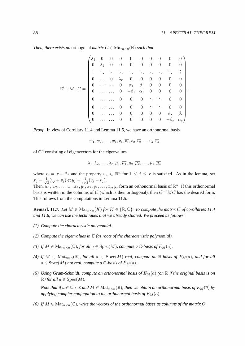
88 11 SPECTRAL THEOREM
Then, there exists anorthogonalmatrixC ∈ Matn×n(R) such that
Ctr ·M · C =
λ1 0 0 0 0 0 0 0 0 0
0 λ2 0 0 0 0 0 0 0 0...
. . . . . . . .. .. . . . . . . . . . . . . ....
0 . . . 0 λr 0 0 0 0 0 0
0 . . . . . . 0 α1 β1 0 0 0 0
0 . . . . . . 0 −β1 α1 0 0 0 0
0 . . . . . . 0 0 0. . . . . . 0 0
0 . . . . . . 0 0 0. . . . . . 0 0
0 . . . . . . 0 0 0 0 0 αs βs0 . . . . . . 0 0 0 0 0 −βs αs
.
Proof. In view of Corollary 11.4 and Lemma 11.5, we have an orthonormal basis
w1, w2, . . . , wr, v1, v1, v2, v2, . . . vs, vs
of Cn consisting of eigenvectors for the eigenvalues
λ1, λ2, . . . , λr, µ1, µ1, µ2, µ2, . . . , µs, µs
wheren = r + 2s and the propertywi ∈ Rn for 1 ≤ i ≤ r is satisfied. As in the lemma, setxj =
1√2(vj + vj) etyj = 1
i√2(vj − vj).
Then,w1, w2, . . . , wr, x1, y1, x2, y2, . . . , xs, ys form an orthonormal basis ofRn. If this orthonormalbasis is written in the columns ofC (which is then orthogonal), thenC−1MC has the desired form.This follows from the computations in Lemma 11.5.
Remark 11.7. LetM ∈ Matn×n(K) for K ∈ {R,C}. To compute the matrixC of corollaries 11.4and 11.6, we can use the techniques that we already studied. We proceedas follows:
(1) Compute the characteristic polynomial.
(2) Compute the eigenvalues inC (as roots of the characteristic polynomial).
(3) If M ∈ Matn×n(C), for all a ∈ Spec(M), compute aC-basis ofEM (a).
(4) If M ∈ Matn×n(R), for all a ∈ Spec(M) real, compute anR-basis ofEM (a), and for alla ∈ Spec(M) not real, compute aC-basis ofEM (a).
(5) Using Gram-Schmidt, compute an orthonormal basis ofEM (a) (onR if the original basis is onR) for all a ∈ Spec(M).
Note that ifa ∈ C \ R andM ∈ Matn×n(R), then we obtain an orthonormal basis ofEM (a) byapplying complex conjugation to the orthonormal basis ofEM (a).
(6) If M ∈ Matn×n(C), write the vectors of the orthonormal bases as columns of the matrixC.

89
(7) If M ∈ Matn×n(R), arrange the eigenvalues ofM (seen as matrix with complex coefficients) asfollows: first the real eigenvaluesλ1, . . . , λr, thenµ1, . . . , µs, µ1, . . . , µs ∈ C \ R.
For each vectorv of the orthonormal basis of a proper spaceEM (µi) for all i = 1, . . . , s, computethe vectorsx, y as in Corollary 11.6 and obtain an orthonormal basis with real coefficientsofEM (µi)⊕ EM (µi).
Write the vectors of the real orthonormal basis ofEM (λi) for i = 1, . . . , r and ofEM (µi) ⊕EM (µi) as columns of the matrixC.
Example 11.8.Let us treat a concrete example for a symmetric matrix. Let
M =
14 38 −40
38 71 20
−40 20 5
.
Its characteristic polynomial is(X + 45)(X − 45)(X − 90).Let us compute the eigenspaces:
EM (−45) = ker
59 38 −40
38 116 20
−40 20 50
= 〈
2
−1
2
〉,
EM (45) = ker
−31 38 −40
38 26 20
−40 20 −40
= 〈
4
−2
−5
〉
and
EM (90) = ker
−76 38 −40
38 −19 20
−40 20 −85
= 〈
1
2
0
〉.
These vectors are already orthogonal by Lemma 11.1. One can easily verify it. Thus, it suffices tonormalize them and to write them as columns of a matrix:
C =
23
43√5
1√5
−13
−23√5
2√5
23
−√5
3 0
.
By construction,C is orthogonal, which can also be checked by a direct computation. We obtain byconstruction (to check by computation):
CtrMC =
−45 0 0
0 45 0
0 0 90
.
We can now state a stronger result ifϕ is self-adjoint.
Corollary 11.9. LetK ∈ {R,C}. LetM ∈ Matn×n(K) be a matrix. Then the following statementsare equivalent:
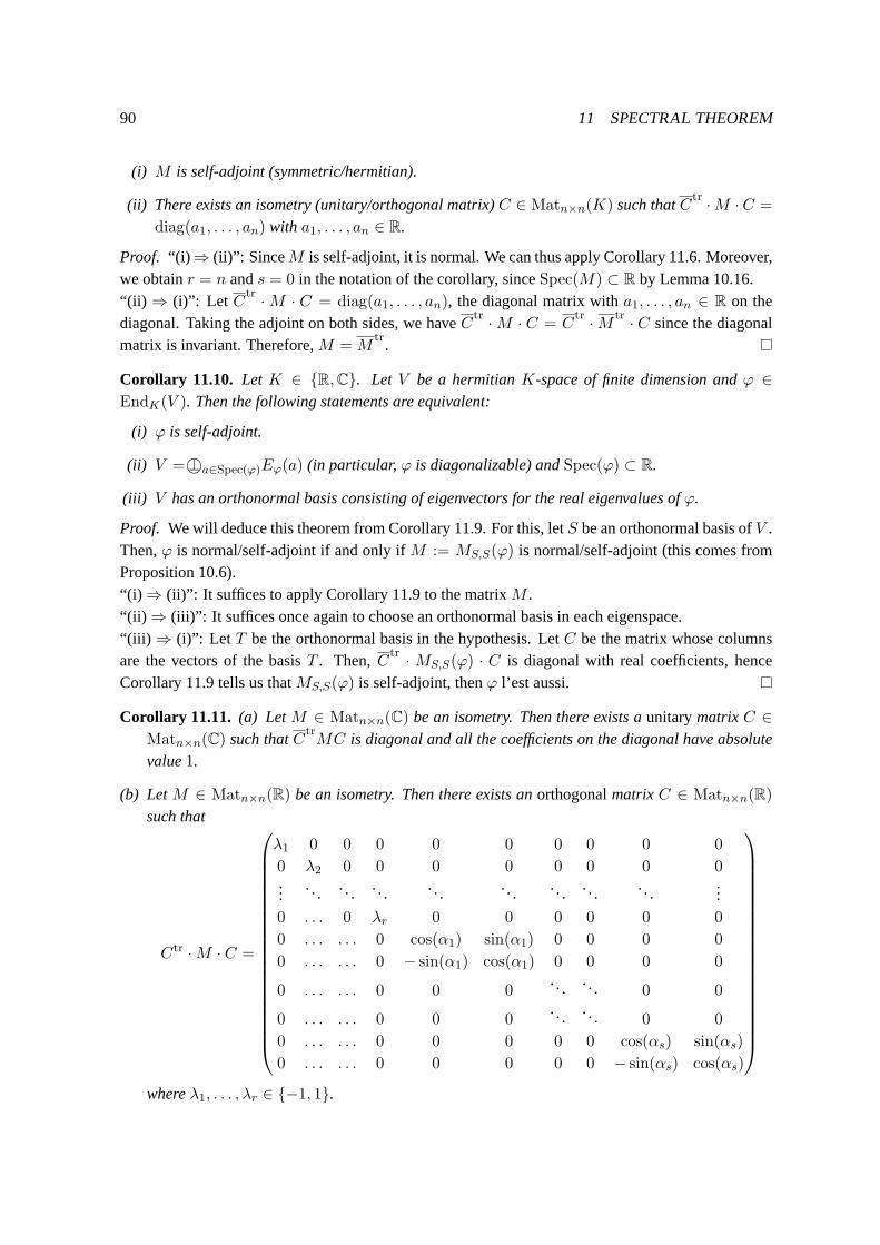
90 11 SPECTRAL THEOREM
(i) M is self-adjoint (symmetric/hermitian).
(ii) There exists an isometry (unitary/orthogonal matrix)C ∈ Matn×n(K) such thatCtr ·M ·C =
diag(a1, . . . , an) with a1, . . . , an ∈ R.
Proof. “(i) ⇒ (ii)”: SinceM is self-adjoint, it is normal. We can thus apply Corollary 11.6. Moreover,we obtainr = n ands = 0 in the notation of the corollary, sinceSpec(M) ⊂ R by Lemma 10.16.“(ii) ⇒ (i)”: Let C
tr ·M · C = diag(a1, . . . , an), the diagonal matrix witha1, . . . , an ∈ R on thediagonal. Taking the adjoint on both sides, we haveC
tr ·M · C = Ctr ·M tr · C since the diagonal
matrix is invariant. Therefore,M =Mtr
.
Corollary 11.10. Let K ∈ {R,C}. Let V be a hermitianK-space of finite dimension andϕ ∈EndK(V ). Then the following statements are equivalent:
(i) ϕ is self-adjoint.
(ii) V =⊥©a∈Spec(ϕ)Eϕ(a) (in particular,ϕ is diagonalizable) andSpec(ϕ) ⊂ R.
(iii) V has an orthonormal basis consisting of eigenvectors for the real eigenvalues ofϕ.
Proof. We will deduce this theorem from Corollary 11.9. For this, letS be an orthonormal basis ofV .Then,ϕ is normal/self-adjoint if and only ifM := MS,S(ϕ) is normal/self-adjoint (this comes fromProposition 10.6).“(i) ⇒ (ii)”: It suffices to apply Corollary 11.9 to the matrixM .“(ii) ⇒ (iii)”: It suffices once again to choose an orthonormal basis in each eigenspace.“(iii) ⇒ (i)”: Let T be the orthonormal basis in the hypothesis. LetC be the matrix whose columnsare the vectors of the basisT . Then,C
tr · MS,S(ϕ) · C is diagonal with real coefficients, henceCorollary 11.9 tells us thatMS,S(ϕ) is self-adjoint, thenϕ l’est aussi.
Corollary 11.11. (a) LetM ∈ Matn×n(C) be an isometry. Then there exists aunitarymatrixC ∈Matn×n(C) such thatC
trMC is diagonal and all the coefficients on the diagonal have absolute
value1.
(b) LetM ∈ Matn×n(R) be an isometry. Then there exists anorthogonalmatrixC ∈ Matn×n(R)such that
Ctr ·M · C =
λ1 0 0 0 0 0 0 0 0 0
0 λ2 0 0 0 0 0 0 0 0...
. .. . .. .. . .. . . . . . . . . . . .. ....
0 . . . 0 λr 0 0 0 0 0 0
0 . . . . . . 0 cos(α1) sin(α1) 0 0 0 0
0 . . . . . . 0 − sin(α1) cos(α1) 0 0 0 0
0 . . . . . . 0 0 0. . . . . . 0 0
0 . . . . . . 0 0 0. . . . . . 0 0
0 . . . . . . 0 0 0 0 0 cos(αs) sin(αs)
0 . . . . . . 0 0 0 0 0 − sin(αs) cos(αs)
whereλ1, . . . , λr ∈ {−1, 1}.
91
Proof. (a) This is an immediate consequence of Corollary 11.4 and of Lemma 10.16.
(b) This follows from Corollary 11.6 and from Lemma 10.16 since forz ∈ C with absolute value1we haveRe(z) = cos(α) andIm(z) = sin(α) if one writesz = exp(iα).
Part (b) is a generalization of Example 10.17.
Corollary 11.12. LetK ∈ {R,C}. LetV be a hermitianK-space of finite dimension and letϕ ∈EndK(V ) be an isometry.
(i) If K = C, then there exists an orthonormalC-basisS of V such thatMS,S(ϕ) is diagonal andall the coefficients on the diagonal have absolute value1.
(ii) If K = R, then there exists an orthonormalC-basisS of V such thatMS,S(ϕ) is as in part (b)of Corollary 11.11.
Proof. Its the translation of Corollary 11.11 in the case of endomorphisms.
Definition 11.13. (a) LetV be a hermitianK-space of finite dimension and letϕ ∈ EndK(V ) au-toadjoint. One says thatϕ is positive (positive definite)if the hermitian form〈, 〉ϕ of Proposi-tion 10.10 is positive (positive definite).
(b) LetM ∈ Matn×n(K) be an autoadjoint (symmetric (ifK = R) or hermitian (ifK = C)) matrix.One says thatM is positive (positive definite)if the hermitian form〈v, w〉M := vtrMw is positive(positive definite).
Lemma 11.14. Let V be a hermitianK-space of finite dimension with orthonormal basisS and letϕ ∈ EndK(V ) be self-adjoint. Then:
(a) ϕ is positive (positive definite)⇐⇒MS,S(ϕ) is positive (positive definite).
(b) ϕ is positive⇐⇒ Spec(ϕ) ⊆ R≥0.
(c) ϕ is positive definite⇐⇒ Spec(ϕ) ⊆ R>0.
Proof. Exercise.
Lemma 11.15.LetM ∈ Matn×n(K) be a positive and self-adjoint matrix (symmetric (ifK = R) orhermitian (ifK = C)). Then there exists a positive matrixN ∈ Matn×n(K) such thatN2 = M andNM =MN . Moreover,M is positive definite if and only ifN is.
Proof. Exercise.
Theorem 11.16(Décomposition polaire). LetV be a hermitianK-space of finite dimension and letϕ ∈ EndK(V ) be an isomorphism (i.e. an invertible endomorphism).
Then there exists a unique autoadjoint and positiveψ ∈ EndK(V ) and a unique isomertyχ ∈EndK(V ) such thatϕ = χ ◦ ψ.
92 12 QUADRICS
Proof. Existence:By one of the exercises,ϕad is also an isomorphism. Define the isomorphismθ := ϕad ◦ ϕ. It is self-adjoint:
θad = (ϕad ◦ ϕ)ad = ϕad ◦ (ϕad)ad = ϕad ◦ ϕ = θ,
henceSpec(θ) ⊆ R by Lemma 10.16. Let us now show that it is positive definite:
〈v, v〉θ = 〈θ(v), v〉 = 〈ϕad(ϕ(v)), v〉 = 〈ϕ(v), ϕ(v)〉 = |ϕ(v)|2 > 0
for all 0 6= v ∈ V . Therefore, by Lemma 11.15 there exists positive definiteψ ∈ EndK(V ) such thatψ2 = θ. Putχ := ϕ ◦ ψ−1. To finish the proof of existence it suffices to prove thatχ is an isomerty:
χ−1 = ψ ◦ ϕ−1 = ψ−1 ◦ ψ2 ◦ ϕ−1 = ψ−1 ◦ θ ◦ ϕ−1
= ψ−1 ◦ ϕad ◦ ϕ ◦ ϕ−1 = ψ−1 ◦ ϕad = (ϕ ◦ ψ−1)ad = χad
where we used(ψ−1)ad = (ψad)−1 = ψ−1 asψ is self-adjoint.
Uniqueness:Assume thatϕ = χ1 ◦ ψ1 = χ2 ◦ ψ2 for isometriesχ1, χ2 and self-adjoint positivedefinite isomorphismsψ1, ψ2. We obtain
χ−12 ◦ χ1 = ψ2 ◦ ψ−1
1 =: β.
On the left hand side we have an isometry and on the right hand side a self-adjoint positive definiteendomorphism. Thus there exists an orthonormal basisS such thatMS,S(β) is diagonal, and thecoefficients on the diagonal are positive reals (sinceβ is positive self-adjoint) and of absolute value1(sinceβ is an isometry). It is therefore the identity,β = id, whenceχ1 = χ2 etψ1 = ψ2.
12 Quadrics
Goals:
• Be able to do simultaneous operations on rows and columns;
• know the link with elementary matrices;
• be able to compute a diagonal matrix using simultaneous operations on rows andcolumns;
• know the definition of quadrics;
• know the definition of equivalence of quadrics;
• know the classification of quadrics;
• be able to compute the type in the classification for a given quadric;
• know examples and be able to prove simple properties.
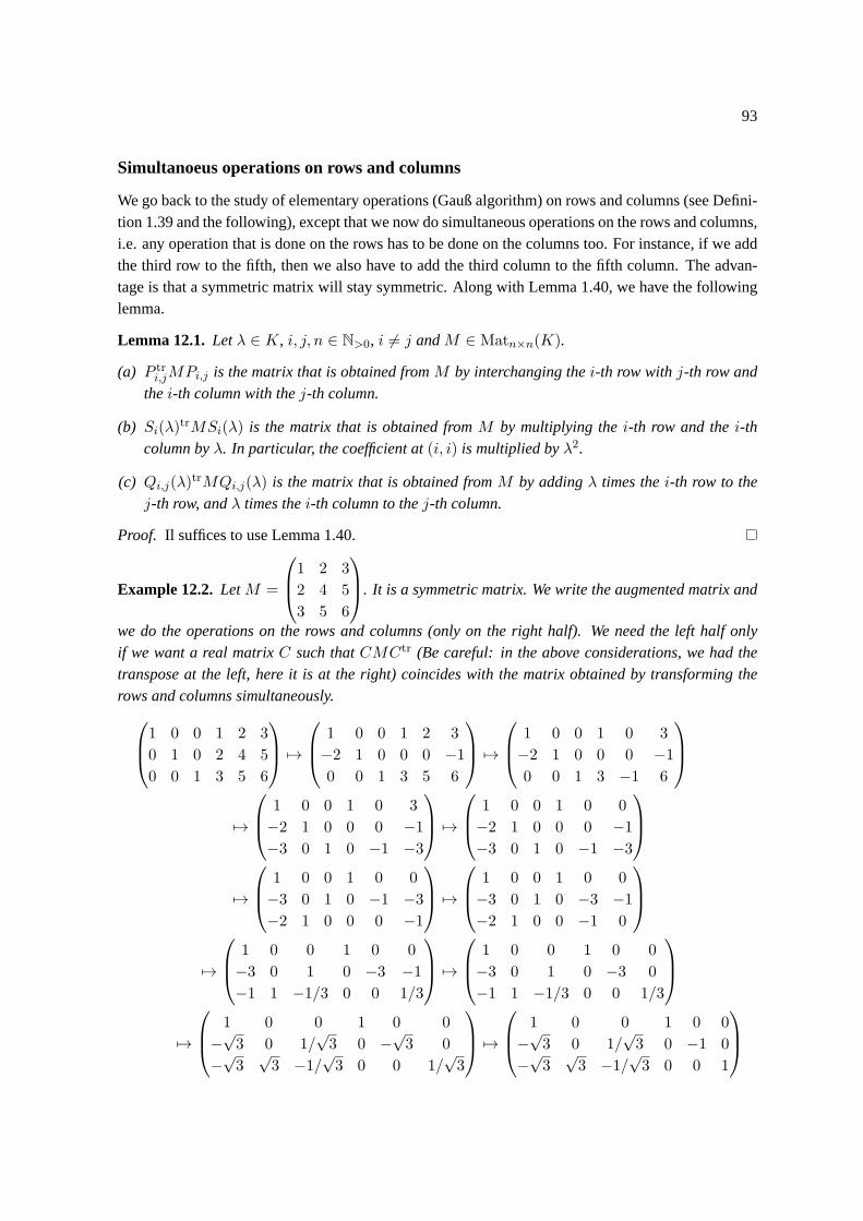
93
Simultanoeus operations on rows and columns
We go back to the study of elementary operations (Gauß algorithm) on rows and columns (see Defini-tion 1.39 and the following), except that we now do simultaneous operations on the rows and columns,i.e. any operation that is done on the rows has to be done on the columns too. For instance, if we addthe third row to the fifth, then we also have to add the third column to the fifth column.The advan-tage is that a symmetric matrix will stay symmetric. Along with Lemma 1.40, we have the followinglemma.
Lemma 12.1. Letλ ∈ K, i, j, n ∈ N>0, i 6= j andM ∈ Matn×n(K).
(a) P tri,jMPi,j is the matrix that is obtained fromM by interchanging thei-th row withj-th row and
thei-th column with thej-th column.
(b) Si(λ)trMSi(λ) is the matrix that is obtained fromM by multiplying thei-th row and thei-thcolumn byλ. In particular, the coefficient at(i, i) is multiplied byλ2.
(c) Qi,j(λ)trMQi,j(λ) is the matrix that is obtained fromM by addingλ times thei-th row to thej-th row, andλ times thei-th column to thej-th column.
Proof. Il suffices to use Lemma 1.40.
Example 12.2.LetM =
1 2 3
2 4 5
3 5 6
. It is a symmetric matrix. We write the augmented matrix and
we do the operations on the rows and columns (only on the right half). We need the left half onlyif we want a real matrixC such thatCMCtr (Be careful: in the above considerations, we had thetranspose at the left, here it is at the right) coincides with the matrix obtained by transforming therows and columns simultaneously.
1 0 0 1 2 3
0 1 0 2 4 5
0 0 1 3 5 6
7→
1 0 0 1 2 3
−2 1 0 0 0 −1
0 0 1 3 5 6
7→
1 0 0 1 0 3
−2 1 0 0 0 −1
0 0 1 3 −1 6
7→
1 0 0 1 0 3
−2 1 0 0 0 −1
−3 0 1 0 −1 −3
7→
1 0 0 1 0 0
−2 1 0 0 0 −1
−3 0 1 0 −1 −3
7→
1 0 0 1 0 0
−3 0 1 0 −1 −3
−2 1 0 0 0 −1
7→
1 0 0 1 0 0
−3 0 1 0 −3 −1
−2 1 0 0 −1 0
7→
1 0 0 1 0 0
−3 0 1 0 −3 −1
−1 1 −1/3 0 0 1/3
7→
1 0 0 1 0 0
−3 0 1 0 −3 0
−1 1 −1/3 0 0 1/3
7→
1 0 0 1 0 0
−√3 0 1/
√3 0 −
√3 0
−√3
√3 −1/
√3 0 0 1/
√3
7→
1 0 0 1 0 0
−√3 0 1/
√3 0 −1 0
−√3
√3 −1/
√3 0 0 1
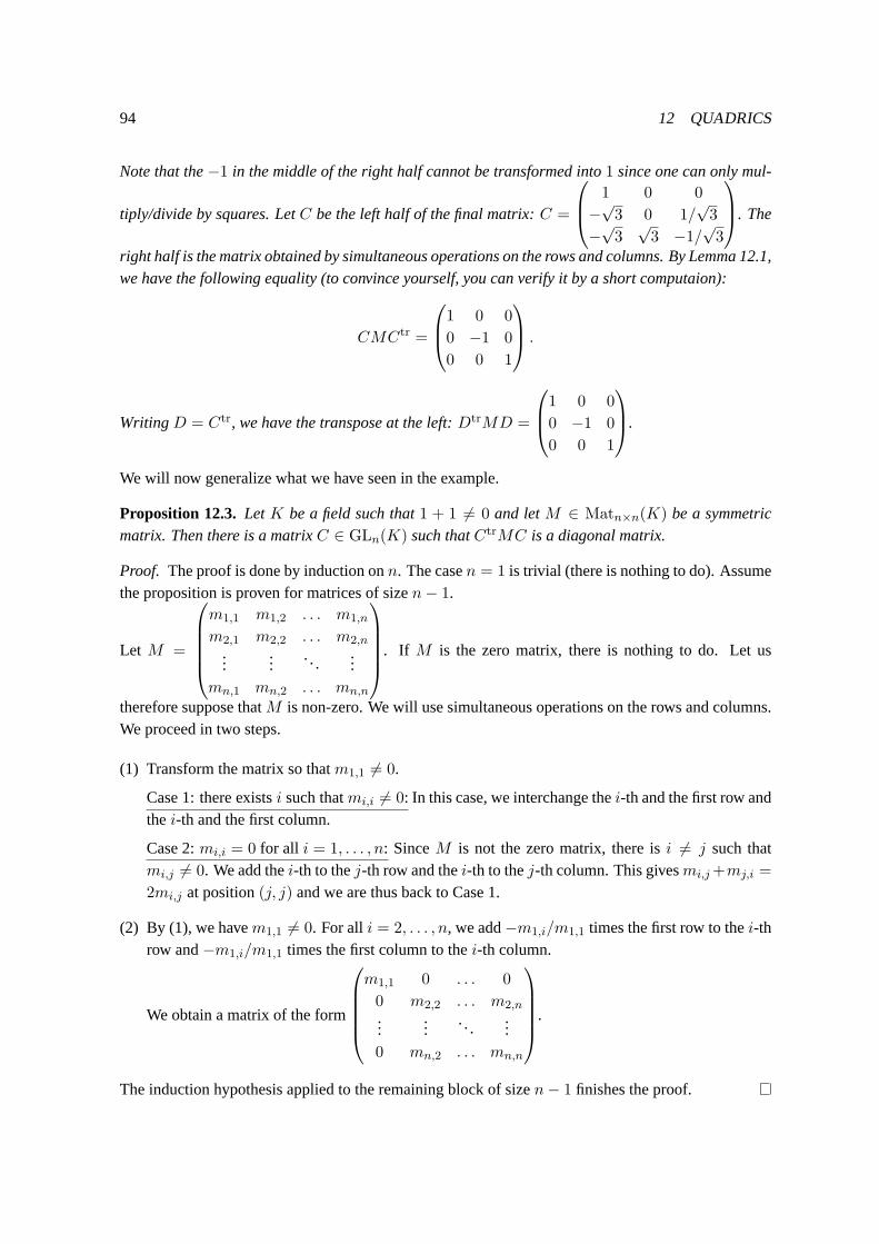
94 12 QUADRICS
Note that the−1 in the middle of the right half cannot be transformed into1 since one can only mul-
tiply/divide by squares. LetC be the left half of the final matrix:C =
1 0 0
−√3 0 1/
√3
−√3
√3 −1/
√3
. The
right half is the matrix obtained by simultaneous operations on the rows and columns. By Lemma 12.1,we have the following equality (to convince yourself, you can verify it by a short computaion):
CMCtr =
1 0 0
0 −1 0
0 0 1
.
WritingD = Ctr, we have the transpose at the left:DtrMD =
1 0 0
0 −1 0
0 0 1
.
We will now generalize what we have seen in the example.
Proposition 12.3. LetK be a field such that1 + 1 6= 0 and letM ∈ Matn×n(K) be a symmetricmatrix. Then there is a matrixC ∈ GLn(K) such thatCtrMC is a diagonal matrix.
Proof. The proof is done by induction onn. The casen = 1 is trivial (there is nothing to do). Assumethe proposition is proven for matrices of sizen− 1.
Let M =
m1,1 m1,2 . . . m1,n
m2,1 m2,2 . . . m2,n...
.... ..
...mn,1 mn,2 . . . mn,n
. If M is the zero matrix, there is nothing to do. Let us
therefore suppose thatM is non-zero. We will use simultaneous operations on the rows and columns.We proceed in two steps.
(1) Transform the matrix so thatm1,1 6= 0.
Case 1: there existsi such thatmi,i 6= 0: In this case, we interchange thei-th and the first row andthei-th and the first column.
Case 2:mi,i = 0 for all i = 1, . . . , n: SinceM is not the zero matrix, there isi 6= j such thatmi,j 6= 0. We add thei-th to thej-th row and thei-th to thej-th column. This givesmi,j+mj,i =
2mi,j at position(j, j) and we are thus back to Case 1.
(2) By (1), we havem1,1 6= 0. For alli = 2, . . . , n, we add−m1,i/m1,1 times the first row to thei-throw and−m1,i/m1,1 times the first column to thei-th column.
We obtain a matrix of the form
m1,1 0 . . . 0
0 m2,2 . . . m2,n...
.... . .
...0 mn,2 . . . mn,n
.
The induction hypothesis applied to the remaining block of sizen− 1 finishes the proof.

95
Corollary 12.4. The rank of a matrix is invariant under simultaneous operations on the rows andcolumns.
Proof. Assume thatN is obtained fromM by simultaneous operations on the rows and columns. ByProposition 12.3 we haveCtrMC = N for an invertible matrixC. SinceCtr is also invertible (forinstance, since0 6= det(C) = det(Ctr)), we haverk(N) = rk(CtrMC) = dim(im(CtrMC)) =
dim(im(CtrM)) = dim(Ctr(im(M)) = dim(im(M)) = rk(M).
Quadrics
In the whole section, letK be a field such that1 + 1 6= 0, for instanceK = R or K = C. Firstrecall thatK[X1, X2, . . . , Xn] denotes the ring of polynomials in variablesX1, X2, . . . , Xn withcoefficients inK. An element ofK[X1, X2, . . . , Xn] is of the form
d1∑
i1=0
d2∑
i2=0
. . .
dn∑
in=0
ai1,i2,...,inXi11 X
i22 . . . Xin
n .
In the sequel, we will only consider quadratic polynomials.
Definition 12.5. We callquadratic polynomial (inn variables and with coefficients inK) any elementofK[X1, X2, . . . , Xn] of the form
q(X1, X2, . . . , Xn) =∑
1≤i≤j≤nai,jXiXj +
n∑
i=1
a0,iXi + a0,0.
Example 12.6. (a) Letn = 1. LetX be the variable. Any quadratic polynomial is of the form
a1,1X2 + a0,1X + a0,0 = a2X
2 + a1X + a0
where we relabelled the coefficients in a standard way.
(b) Letn = 2. LetX,Y be the variables. Any quadratic polynomial is of the form
a1,1X2 + a1,2XY + a2,2Y
2 + a0,1X + a0,2Y + a0,0.
In particular, we have the following example:
(1) X2
a2+ Y 2
b2− 1
(2) X2
a2− Y 2
b2− 1
(3) X2
a2− Y
Lemma 12.7.Letn ∈ N and letA ∈ Mat(n+1)×(n+1)(K) be a symmetricmatrix. Its coefficients willbe calledai,j for 0 ≤ i, j ≤ n (note that the numeration starts at0!). Let X be the vector containingthe variables preceded by1:
A =
a0,0 a0,1 . . . a0,na0,1 a1,1 . . . a1,n
......
. . ....
a0,n a1,n . . . an,n
, X =
1
X1...Xn
.

96 12 QUADRICS
Then the polynomial
qA(X1, . . . , Xn) = XtrAX = 2∑
1≤i<j≤nai,jXiXj +
n∑
i=1
ai,iX2i + 2
n∑
i=1
a0,iXi + a0,0
is quadratic and any quadratic polynomial arises from a unique symmetric matrix A by this formula.
Proof. Clear.
As in the preceding lemma, forx =
( x1...xn
)∈ Kn, we denotex =
1x1...xn
, the vectorx preceded
by 1.
Definition 12.8. We callquadric (in dimensionn) any set
QA := QA(K) := {x ∈ Kn | xtrAx = 0}
whereA is a symmetric matrixMat(n+1)×(n+1)(K).
Example 12.9.Considern = 2.
(1) LetA =
−1 0 0
0 1a2
0
0 0 1b2
. We haveQA = {x ∈ R2 | X2
a2+ Y 2
b2− 1 = 0}. Geometrically, it
defines an ellipse.
(2) LetA =
−1 0 0
0 1a2
0
0 0 −1b2
. We haveQA = {x ∈ R2 | X2
a2− Y 2
b2− 1 = 0}. Geometrically, it
defines a hyperbola.
(3) LetA =
0 0 −12
0 1a2
0−12 0 0
. We haveQA = {x ∈ R2 | X2
a2− Y = 0}. Geometrically, it defines a
parabola.
We also define an augmented matrix: letC = (ci,j) ∈ Matn×n(K) be a matrix andy ∈ Kn a vector.We set:
Cy =
1 0 . . . 0
y1 c1,1 . . . c1,n...
.... . .
...yn cn,1 . . . cn,n
.
Lemma 12.10.LetA ∈ Mat(n+1)×(n+1)(K) be a symmetric matrix andQA the associated quadric.Letϕ : Kn → Kn be anaffinity, i.e. an application of the form
ϕ(v) = Bv +By
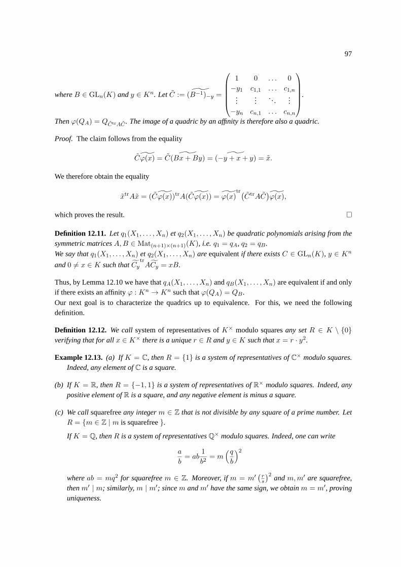
97
whereB ∈ GLn(K) andy ∈ Kn. Let C := ˜(B−1)−y =
1 0 . . . 0
−y1 c1,1 . . . c1,n...
.... ..
...−yn cn,1 . . . cn,n
.
Thenϕ(QA) = QCtrAC . The image of a quadric by an affinity is therefore also a quadric.
Proof. The claim follows from the equality
Cϕ(x) = C ˜(Bx+By) = ˜(−y + x+ y) = x.
We therefore obtain the equality
xtrAx = (Cϕ(x))trA(Cϕ(x)) = ϕ(x)tr(CtrAC
)ϕ(x),
which proves the result.
Definition 12.11. Let q1(X1, . . . , Xn) et q2(X1, . . . , Xn) be quadratic polynomials arising from thesymmetric matricesA,B ∈ Mat(n+1)×(n+1)(K), i.e. q1 = qA, q2 = qB.
We say thatq1(X1, . . . , Xn) et q2(X1, . . . , Xn) are equivalentif there existsC ∈ GLn(K), y ∈ Kn
and0 6= x ∈ K such thatCytrACy = xB.
Thus, by Lemma 12.10 we have thatqA(X1, . . . , Xn) andqB(X1, . . . , Xn) are equivalent if and onlyif there exists an affinityϕ : Kn → Kn such thatϕ(QA) = QB.
Our next goal is to characterize the quadrics up to equivalence. For this, we need the followingdefinition.
Definition 12.12. We callsystem of representatives ofK× modulo squaresany setR ∈ K \ {0}verifying that for allx ∈ K× there is a uniquer ∈ R andy ∈ K such thatx = r · y2.
Example 12.13.(a) If K = C, thenR = {1} is a system of representatives ofC× modulo squares.Indeed, any element ofC is a square.
(b) If K = R, thenR = {−1, 1} is a system of representatives ofR× modulo squares. Indeed, anypositive element ofR is a square, and any negative element is minus a square.
(c) We callsquarefreeany integerm ∈ Z that is not divisible by any square of a prime number. LetR = {m ∈ Z | m is squarefree}.
If K = Q, thenR is a system of representativesQ× modulo squares. Indeed, one can write
a
b= ab
1
b2= m
(qb
)2
whereab = mq2 for squarefreem ∈ Z. Moreover, ifm = m′ ( rs
)2andm,m′ are squarefree,
thenm′ | m; similarly,m | m′; sincem andm′ have the same sign, we obtainm = m′, provinguniqueness.
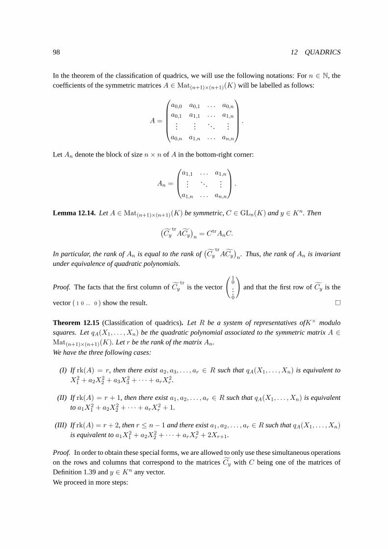
98 12 QUADRICS
In the theorem of the classification of quadrics, we will use the following notations: Forn ∈ N, thecoefficients of the symmetric matricesA ∈ Mat(n+1)×(n+1)(K) will be labelled as follows:
A =
a0,0 a0,1 . . . a0,na0,1 a1,1 . . . a1,n
......
.. ....
a0,n a1,n . . . an,n
.
LetAn denote the block of sizen× n of A in the bottom-right corner:
An =
a1,1 . . . a1,n
.... ..
...a1,n . . . an,n
.
Lemma 12.14.LetA ∈ Mat(n+1)×(n+1)(K) be symmetric,C ∈ GLn(K) andy ∈ Kn. Then
(Cy
trACy
)n= CtrAnC.
In particular, the rank ofAn is equal to the rank of(Cy
trACy
)n. Thus, the rank ofAn is invariant
under equivalence of quadratic polynomials.
Proof. The facts that the first column ofCytr
is the vector
( 10...0
)and that the first row ofCy is the
vector( 1 0 ... 0 ) show the result.
Theorem 12.15(Classification of quadrics). Let R be a system of representatives ofK× modulosquares. LetqA(X1, . . . , Xn) be the quadratic polynomial associated to the symmetric matrixA ∈Mat(n+1)×(n+1)(K). Letr be the rank of the matrixAn.
We have the three following cases:
(I) If rk(A) = r, then there exista2, a3, . . . , ar ∈ R such thatqA(X1, . . . , Xn) is equivalent toX2
1 + a2X22 + a3X
23 + · · ·+ arX
2r .
(II) If rk(A) = r + 1, then there exista1, a2, . . . , ar ∈ R such thatqA(X1, . . . , Xn) is equivalentto a1X2
1 + a2X22 + · · ·+ arX
2r + 1.
(III) If rk(A) = r+ 2, thenr ≤ n− 1 and there exista1, a2, . . . , ar ∈ R such thatqA(X1, . . . , Xn)
is equivalent toa1X21 + a2X
22 + · · ·+ arX
2r + 2Xr+1.
Proof. In order to obtain these special forms, we are allowed to only use these simultaneous operationson the rows and columns that correspond to the matricesCy with C being one of the matrices ofDefinition 1.39 andy ∈ Kn any vector.
We proceed in more steps:
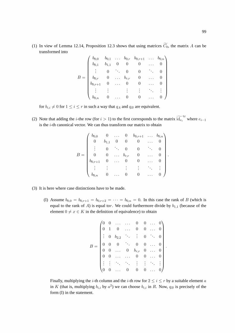
99
(1) In view of Lemma 12.14, Proposition 12.3 shows that using matricesC0, the matrixA can betransformed into
B =
b0,0 b0,1 . . . b0,r b0,r+1 . . . b0,nb0,1 b1,1 0 0 0 . . . 0
... 0. . . 0 0
. .. 0
b0,r 0 . . . br,r 0 . . . 0
b0,r+1 0 . . . 0 0 . . . 0...
......
.... ..
...b0,n 0 . . . 0 0 . . . 0
for bi,i 6= 0 for 1 ≤ i ≤ r in such a way thatqA andqB are equivalent.
(2) Note that adding thei-the row (fori > 1) to the first corresponds to the matrixideitr
whereei−1
is thei-th canonical vector. We can thus transform our matrix to obtain
B =
b0,0 0 . . . 0 b0,r+1 . . . b0,n0 b1,1 0 0 0 . . . 0... 0
. .. 0 0.. . 0
0 0 . . . br,r 0 . . . 0
b0,r+1 0 . . . 0 0 . . . 0...
......
..... .
...b0,n 0 . . . 0 0 . . . 0
.
(3) It is here where case distinctions have to be made.
(I) Assumeb0,0 = b0,r+1 = b0,r+2 = · · · = b0,n = 0. In this case the rank ofB (which isequal to the rank ofA) is equal tor. We could furthermore divide byb1,1 (because of theelement0 6= x ∈ K in the definition of equivalence) to obtain
B =
0 0 . . . . . . 0 0 . . . 0
0 1 0 . . . 0 0 . . . 0... 0 b2,2
. . .... 0
.. . 0
0 0 0. . . 0 0 . . . 0
0 0 . . . 0 br,r 0 . . . 0
0 0 . . . . . . 0 0 . . . 0...
..... . . . .
......
.. ....
0 0 . . . 0 0 0 . . . 0
.
Finally, multiplying thei-th column and thei-th row for2 ≤ i ≤ r by a suitable elementain K (that is, multiplyingbi,i by a2) we can choosebi,i in R. Now, qB is precisely of theform (I) in the statement.
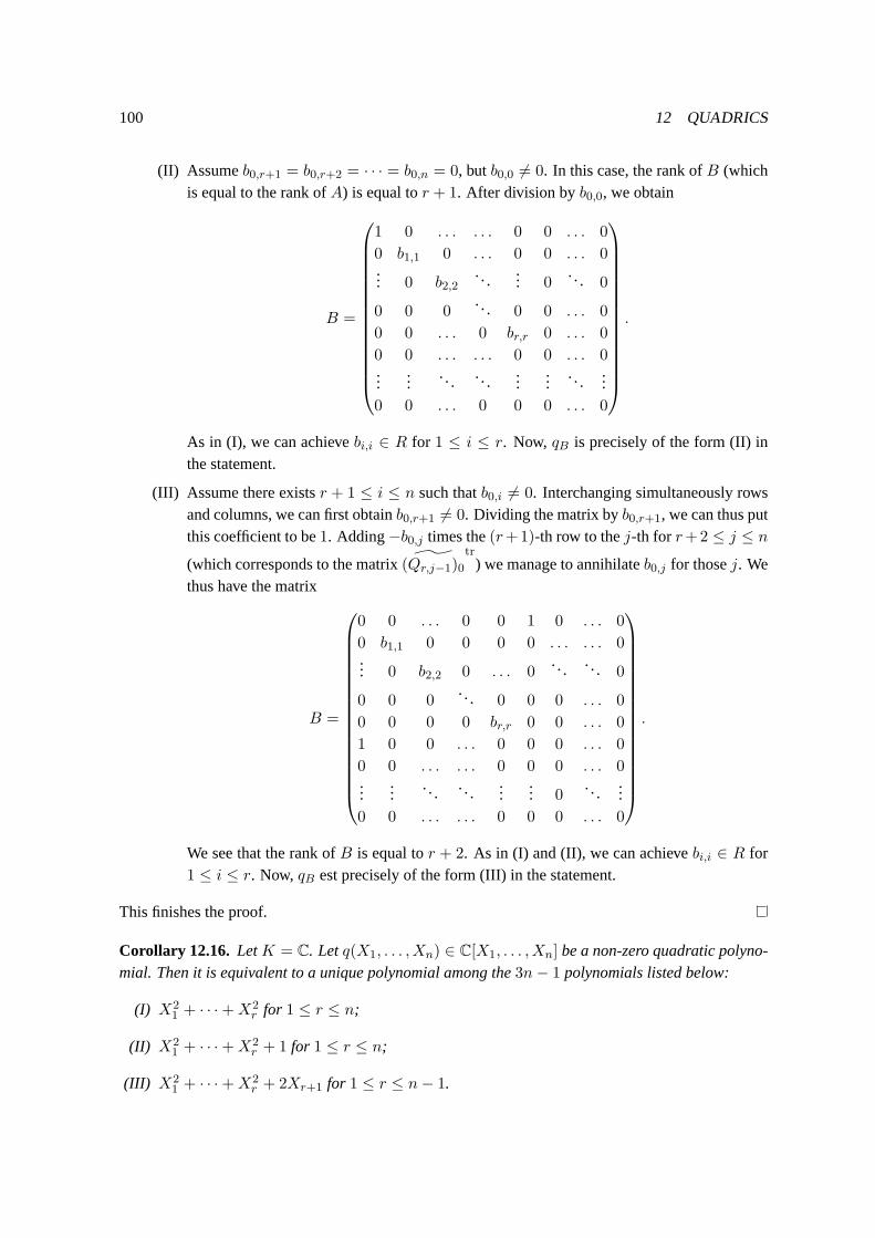
100 12 QUADRICS
(II) Assumeb0,r+1 = b0,r+2 = · · · = b0,n = 0, butb0,0 6= 0. In this case, the rank ofB (whichis equal to the rank ofA) is equal tor + 1. After division byb0,0, we obtain
B =
1 0 . . . . . . 0 0 . . . 0
0 b1,1 0 . . . 0 0 . . . 0... 0 b2,2
. . .... 0
.. . 0
0 0 0. . . 0 0 . . . 0
0 0 . . . 0 br,r 0 . . . 0
0 0 . . . . . . 0 0 . . . 0...
.... . . . . .
......
.. ....
0 0 . . . 0 0 0 . . . 0
.
As in (I), we can achievebi,i ∈ R for 1 ≤ i ≤ r. Now, qB is precisely of the form (II) inthe statement.
(III) Assume there existsr + 1 ≤ i ≤ n such thatb0,i 6= 0. Interchanging simultaneously rowsand columns, we can first obtainb0,r+1 6= 0. Dividing the matrix byb0,r+1, we can thus putthis coefficient to be1. Adding−b0,j times the(r+1)-th row to thej-th for r+2 ≤ j ≤ n
(which corresponds to the matrix(Qr,j−1)0tr
) we manage to annihilateb0,j for thosej. Wethus have the matrix
B =
0 0 . . . 0 0 1 0 . . . 0
0 b1,1 0 0 0 0 . . . . . . 0... 0 b2,2 0 . . . 0
. .. . . . 0
0 0 0. .. 0 0 0 . . . 0
0 0 0 0 br,r 0 0 . . . 0
1 0 0 . . . 0 0 0 . . . 0
0 0 . . . . . . 0 0 0 . . . 0...
.... .. . ..
...... 0
. . ....
0 0 . . . . . . 0 0 0 . . . 0
.
We see that the rank ofB is equal tor + 2. As in (I) and (II), we can achievebi,i ∈ R for1 ≤ i ≤ r. Now, qB est precisely of the form (III) in the statement.
This finishes the proof.
Corollary 12.16. LetK = C. Letq(X1, . . . , Xn) ∈ C[X1, . . . , Xn] be a non-zero quadratic polyno-mial. Then it is equivalent to a unique polynomial among the3n− 1 polynomials listed below:
(I) X21 + · · ·+X2
r for 1 ≤ r ≤ n;
(II) X21 + · · ·+X2
r + 1 for 1 ≤ r ≤ n;
(III) X21 + · · ·+X2
r + 2Xr+1 for 1 ≤ r ≤ n− 1.
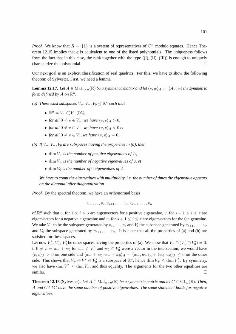
101
Proof. We know thatR = {1} is a system of representatives ofC× modulo squares. Hence The-orem 12.15 implies thatq is equivalent to one of the listed polynomials. The uniqueness followsfrom the fact that in this case, the rank together with the type ((I), (II), (III)) is enough to uniquelycharacterize the polynomial.
Our next goal is an explicit classification of real quadrics. For this, we have to show the followingtheorem of Sylvester. First, we need a lemma.
Lemma 12.17.LetA ∈ Matn×n(R) be a symmetric matrix and let〈v, w〉A := 〈Av,w〉 the symmetricform defined byA onRn.
(a) There exist subspacesV+, V−, V0 ≤ Rn such that
• Rn = V+ ⊥©V− ⊥©V0,
• for all 0 6= v ∈ V+, we have〈v, v〉A > 0,
• for all 0 6= v ∈ V−, we have〈v, v〉A < 0 et
• for all 0 6= v ∈ V0, we have〈v, v〉A = 0.
(b) If V+, V−, V0 are subspaces having the properties in (a), then
• dimV+ is the number of positive eigenvalues ofA,
• dimV− is the number of negative eigenvalues ofA et
• dimV0 is the number of0 eigenvalues ofA.
We have to count the eigenvalues with multiplicity, i.e. the number of times the eigenvalue appearson the diagonal after diagonalization.
Proof. By the spectral theorem, we have an orthonormal basis
v1, . . . , vs, vs+1, . . . , vr, vr+1, . . . , vn
of Rn such thatvi for 1 ≤ i ≤ s are eigenvectors for a positive eigenvalue,vi for s + 1 ≤ i ≤ r areeigenvectors for a negative eigenvalue andvi for s+ 1 ≤ i ≤ r are eigenvectors for the0 eigenvalue.We takeV+ to be the subspace generated byv1, . . . , vs andVi the subspace generated byvs+1, . . . , vrandV0 the subspace generated byvr+1, . . . , vn. It is clear that all the properties of (a) and (b) aresatisfied for these spaces.Let nowV ′
+, V ′−, V ′
0 be other spaces having the properties of (a). We show thatV+ ∩ (V ′− ⊕ V ′
0) = 0:if 0 6= v = w− + w0 for w− ∈ V ′
− andw0 ∈ V ′0 were a vector in the intersection, we would have
〈v, v〉A > 0 on one side and〈w− + w0, w− + w0〉A = 〈w−, w−〉A + 〈w0, w0〉A ≤ 0 on the otherside. This shows thatV+ ⊕ V ′
− ⊕ V ′0 is a subspace ofRn, hencedimV+ ≤ dimV ′
+. By symmetry,we also havedimV ′
+ ≤ dimV+, and thus equality. The arguments for the two other equalities aresimilar.
Theorem 12.18(Sylvester). LetA ∈ Matn×n(R) be a symmetric matrix and letC ∈ GLn(R). Then,A andCtrAC have the same number of positive eigenvalues. The same statement holdsfor negativeeigenvalues.
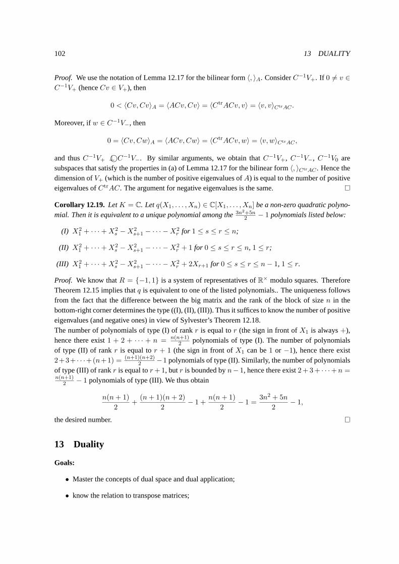
102 13 DUALITY
Proof. We use the notation of Lemma 12.17 for the bilinear form〈, 〉A. ConsiderC−1V+. If 0 6= v ∈C−1V+ (henceCv ∈ V+), then
0 < 〈Cv,Cv〉A = 〈ACv,Cv〉 = 〈CtrACv, v〉 = 〈v, v〉CtrAC .
Moreover, ifw ∈ C−1V−, then
0 = 〈Cv,Cw〉A = 〈ACv,Cw〉 = 〈CtrACv,w〉 = 〈v, w〉CtrAC ,
and thusC−1V+ ⊥©C−1V−. By similar arguments, we obtain thatC−1V+, C−1V−, C−1V0 aresubspaces that satisfy the properties in (a) of Lemma 12.17 for the bilinear form 〈, 〉CtrAC . Hence thedimension ofV+ (which is the number of positive eigenvalues ofA) is equal to the number of positiveeigenvalues ofCtrAC. The argument for negative eigenvalues is the same.
Corollary 12.19. LetK = C. Letq(X1, . . . , Xn) ∈ C[X1, . . . , Xn] be a non-zero quadratic polyno-mial. Then it is equivalent to a unique polynomial among the3n2+5n
2 − 1 polynomials listed below:
(I) X21 + · · ·+X2
s −X2s+1 − · · · −X2
r for 1 ≤ s ≤ r ≤ n;
(II) X21 + · · ·+X2
s −X2s+1 − · · · −X2
r + 1 for 0 ≤ s ≤ r ≤ n, 1 ≤ r;
(III) X21 + · · ·+X2
s −X2s+1 − · · · −X2
r + 2Xr+1 for 0 ≤ s ≤ r ≤ n− 1, 1 ≤ r.
Proof. We know thatR = {−1, 1} is a system of representatives ofR× modulo squares. ThereforeTheorem 12.15 implies thatq is equivalent to one of the listed polynomials.. The uniqueness followsfrom the fact that the difference between the big matrix and the rank of the block of sizen in thebottom-right corner determines the type ((I), (II), (III)). Thus it suffices to know the number of positiveeigenvalues (and negative ones) in view of Sylvester’s Theorem 12.18.The number of polynomials of type (I) of rankr is equal tor (the sign in front ofX1 is always+),hence there exist1 + 2 + · · · + n = n(n+1)
2 polynomials of type (I). The number of polynomialsof type (II) of rankr is equal tor + 1 (the sign in front ofX1 can be1 or −1), hence there exist2+3+ · · ·+(n+1) = (n+1)(n+2)
2 −1 polynomials of type (II). Similarly, the number of polynomialsof type (III) of rankr is equal tor+1, butr is bounded byn− 1, hence there exist2+3+ · · ·+n =n(n+1)
2 − 1 polynomials of type (III). We thus obtain
n(n+ 1)
2+
(n+ 1)(n+ 2)
2− 1 +
n(n+ 1)
2− 1 =
3n2 + 5n
2− 1,
the desired number.
13 Duality
Goals:
• Master the concepts of dual space and dual application;
• know the relation to transpose matrices;
103
• know the definition and fundamental properties of bilinear forms;
• know the relation to the rank of rows and columns of matrices;
• know examples and be able to prove simple properties.
In this section, we introduce a theory of duality, that is valid for any fieldK (not only forR andC).The main results of this section are
• the interpretation of transpose matrices as matrices representing “dual” applications;
• the rank of the columns of a matrix is equal to the rank of the rows; this is sometimesuseful forcomputations.
We start with the interpretation of transpose matrices as matrices representingdual applications. Forthis, we first introduce the dual vector spacelV ∗ of a vector spaceV .
Lemma 13.1. LetV,W be twoK-vector spaces.
(a) The set ofK-linear applications
HomK(V,W ) := {f : V →W | f isK-linear}
is aK-vector space for the addition
(f + g)(v) := f(v) + g(v) for f, g ∈ HomK(V,W ) andv ∈ V
and the scalar multiplication
(x.f)(v) := x.(f(v)) = f(x.v) for f ∈ HomK(V,W ), x ∈ K andv ∈ V.
(b) Let S be aK-basis ofV and f : S → W be an application. Then, there exists a uniqueF ∈ HomK(V,W ) such thatF |S = f , namelyF (
∑s∈S ass) =
∑s∈S asf(s).
Proof. Simple computations.
Definition 13.2. LetV be aK-vector space. TheK-vector space (see Lemma 13.1(a))
V ∗ := HomK(V,K)
is called thedual space ofV .
Proposition 13.3. LetV be aK-vector space of finite dimensionn.
(a) LetS = {s1, . . . , sn} be aK-basis ofV . For all 1 ≤ i ≤ n, let s∗i be the unique (by Lemma
13.1(b)) element inV ∗ such that for all1 ≤ j ≤ n we haves∗i (sj) = δi,j =
{1 if i = j,
0 if i 6= j.
Then,S∗ := {s∗1, . . . , s∗n} is aK-basis ofV ∗, called thedual basis.
(b) If V has finiteK-dimension, thendimK(V∗) = dimK(V ).
104 13 DUALITY
Proof. (a) Linear independence:Let 0 =∑n
i=1 ais∗i with a1, . . . , an ∈ K. Then, for all1 ≤ j ≤ n
we have
0 =n∑
i=1
ais∗i (sj) =
n∑
i=1
aiδi,j = aj .
Generating:Let f ∈ V ∗. For1 ≤ j ≤ n, setaj := f(sj) andg :=∑n
i=1 ais∗i ∈ V ∗. We have
g(sj) =
n∑
i=1
ais∗i (sj) = aj = f(sj)
for all 1 ≤ j ≤ n, thusf = g.(b) The dimension ofV is the cardinality of any basis ofV . By (a), the dual basis has the samecardinality as any basis ofV , thus the dimension ofV ∗ equals the dimension ofV .
Definition-Lemma 13.4. LetV,W be twoK-vector spaces andϕ : V →W be aK-linear applica-tion. Then, the application
ϕ∗ :W ∗ → V ∗, f 7→ ϕ∗(f) = f ◦ ϕ
isK-linear. It is called thedual application ofϕ.
Proof. Firstly we note thatϕ◦f isK-linear; but, this follows from the fact that the composition of twolinear applications is linear. Letf, g ∈W ∗ andx ∈ K. We conclude the proof by the computation
ϕ∗(x · f + g)(v) = ((x · f + g) ◦ ϕ)(v) = (x · f + g)(ϕ(v))
= xf(ϕ(v)) + g(ϕ(v)) = (xϕ∗(f) + ϕ∗(g))(v).
for anyv ∈ V , whenceϕ∗(x · f + g) = xϕ∗(f) + ϕ∗(g).
Proposition 13.5. LetV,W be twoK-vector spaces andϕ : V →W be aK-linear application. LetmoreoverS = {s1, . . . , sn} be aK-basis ofV andT = {t1, . . . , tm} aK-basis ofW . Then,
(MT,S(ϕ)
)tr=MS∗,T ∗(ϕ∗).
Thus, the matrix representingϕ∗ for the dual bases is the transpose of the matrix representingϕ.
Proof. We write
MT,S(ϕ) =
a1,1 a1,2 · · · a1,na2,1 a2,2 · · · a2,n
......
. . ....
am,1 am,2 · · · am,n
andMS∗,T ∗(ϕ∗) =
b1,1 b1,2 · · · b1,mb2,1 b2,2 · · · b2,m
......
. . ....
bn,1 bn,2 · · · bn,m
.
This means
ϕ(sj) =m∑
i=1
ai,jti andϕ∗(t∗k) =n∑
i=1
bi,ks∗i
105
for all 1 ≤ j ≤ n and1 ≤ k ≤ m. Thus, on the one hand
(ϕ∗(t∗k))(sj) = t∗k(ϕ(sj)) = t∗k(m∑
i=1
ai,jti) =m∑
i=1
ai,jt∗k(ti) = ak,j
and on the other hand
(ϕ∗(t∗k))(sj) =n∑
i=1
bi,ks∗i (sj) = bj,k,
whenceak,j = bj,k, as desired.
The dual space gives rise to a natural bilinear form, as we will see in Example 13.8(b); first we makethe necessary definitions.
Definition 13.6. LetV,W be twoK-vector spaces. One callsbilinear formany application
〈·, ·〉 : V ×W → K
such that
• ∀ a ∈ K ∀ v1, v2 ∈ V ∀w ∈ W : 〈av1 + v2, w〉 = a〈v1, w〉 + 〈v2, w〉 (linearity in the firstvariable) and
• ∀ b ∈ K ∀ v ∈ V ∀w1, w2 ∈ W : 〈v, bw1 + w2〉 = b〈v, w1〉+ 〈v, w2〉 (linearity in the secondvariable).
Let 〈·, ·〉 : V ×W → K be a bilinear form. For a subspaceV1 ≤ V , we call
V ⊥1 := {w ∈W | ∀v ∈ V1 : 〈v, w〉 = 0} ≤W
theorthogonal complement ofV1 in W .For a subspaceW1 ≤W , we call
W⊥1 := {v ∈ V | ∀w ∈W1 : 〈v, w〉 = 0} ≤ V
theorthogonal complement ofW1 in V .We say that the bilinear formis non-degenerateif
• ∀ 0 6= v ∈ V ∃w ∈W : 〈v, w〉 6= 0 and
• ∀ 0 6= w ∈W ∃ v ∈ V : 〈v, w〉 6= 0.
In the sequel, we will write〈v,W1〉 = 0 for ∀w ∈W1 : 〈v, w〉 = 0 (and vice-versa).
Lemma 13.7. LetV,W be twoK-vector spaces and〈·, ·〉 : V ×W → K be a bilinear form.
(a) For any subspaceV1 ≤ V , the orthogonal complement ofV1 in W is a subspace ofW and forany subspaceW1 ≤W , the orthogonal complement ofW1 in V is a subspace ofV .
(b) LetW1 ≤W2 ≤W be two subspaces. Then,W⊥2 ≤W⊥
1 .
Also: V ⊥2 ≤ V ⊥
1 for any subspacesV1 ≤ V2 ≤ V .
106 13 DUALITY
(c) The bilinear form is non-degenerate if and only ifW⊥ = 0 andV ⊥ = 0.
Proof. (a) LetV1 ≤ V be a subspace. Letw1, w2 ∈ V ⊥1 , i.e.,〈v, wi〉 = 0 for i = 1, 2 and allv ∈ V1.
Thus, for alla ∈ K we have the equality
〈v, aw1 + w2〉 = a〈v, w1〉+ 〈v, w2〉 = 0,
whenceaw1 + w2 ∈ V ⊥1 . The argument forW⊥
1 is the same.(b) Let v ∈ W⊥
2 . By definition 〈v,W2〉 = 0, hence in particular〈v,W1〉 = 0, i.e. v ∈ W⊥1 . The
second statement follows by the same argument.(c) This is another way of writing the definition.
Example 13.8. (a) The application
〈·, ·〉 : Kn ×Kn → K, 〈
a1a2...an
,
b1b2...bn
〉 =
(a1 a2 . . . an
)
b1b2...bn
=n∑
i=1
aibi
is bilinear and non-degenerate.
(b) LetV be aK-vector space of finite dimension. The application
〈·, ·〉 : V ∗ × V → K, 〈f, v〉 := f(v)
is bilinear and non-degenerate.
LetS = {s1, . . . , sn} be aK-basis ofV andS∗ the dual basis. Letf =∑n
i=1 ais∗i ∈ V ∗ and
v =∑n
i=1 bisi ∈ V . Then
〈f, v〉 = 〈n∑
i=1
ais∗i ,
n∑
j=1
bjsj〉 =n∑
i=1
n∑
j=1
aibj〈s∗i , sj〉 =n∑
i=1
n∑
j=1
aibjs∗i (sj)
=n∑
i=1
aibi =(a1 a2 . . . an
)
b1b2...bn
.
We have found the bilinearity of (a).
Proposition 13.9. LetV,W be twoK-vector spaces of finite dimensions and〈·, ·〉 : V ×W → K bea non-degenerate bilinear form.
(a) The applications
ϕ : V →W ∗, v 7→ ϕ(v) =: ϕv with ϕv(w) := 〈v, w〉,
andψ :W → V ∗, w 7→ ψ(w) =: ψw with ψw(v) := 〈v, w〉
areK-linear isomorphisms.
107
(b) dimK(V ) = dimK(W ).
Proof. TheK-linearity ofϕ andψ is clear. We show the injectivity ofϕ. For this, letv ∈ ker(ϕ),i.e.,ϕv(w) = 〈v, w〉 = 0 for all w ∈W . The non-degeneracy of the bilinear form implies thatv = 0,which proves the injectivity. From this we deducedimK(V ) ≤ dimK(W ∗) = dimK(W ).The same arguments applies toψ give thatψ is injective and thusdimK(W ) ≤ dimK(V
∗) =
dimK(V ), d’où dimK(V ) = dimK(W ). Consequently,ϕ andψ are isomorphisms (because thedimension of the image is equal to the dimension of the target space which are thus equal).
Corollary 13.10. LetV,W be twoK-vector spaces of finite dimensions.
(a) Then, the application
ψ : V → (V ∗)∗, v 7→ ψv = evv : V∗ → K whereψv(f) = evv(f) = f(v) for f ∈ V ∗
is aK-linear isomorphism.
(b) Letα : V →W be aK-linear application. Then, the diagram
Vα
//
ψ1
��
W
ψ2
��
(V ∗)∗(α∗)∗
// (W ∗)∗.
is commutative, whereψ1 andψ2 are the isomorphisms from (a), i.e.ψ2 ◦ α = (α∗)∗ ◦ ψ1.
(c) Lett1, . . . , tn be aK-basis ofV ∗. Then, there exists aK-basiss1, . . . , sn ofV such thatti(sj) =δi,j for all 1 ≤ i, j ≤ n.
Proof. (a) The bilinear formV ∗ × V → K, given by〈f, v〉 7→ f(v) from Example 13.8(b) is non-degenerate. The applicationψ is theψ of Proposition 13.9.(b) Let v ∈ V . On the one hand, we have(α∗)∗(ψ1(v)) = (α∗)∗(evv) = evv ◦ α∗ and on the otherhandψ2(α(v)) = evα(v) with notations from (a). To see that both are equal, letf ∈W ∗. We have
evv(α∗(f)) = evv(f ◦ α) = f(α(v)) andevα(v)(f) = f(α(v)),
thus the desired equality.(c) Let t∗1, . . . , t
∗n ∈ (V ∗)∗ be the dual basis, i.e.t∗j (ti) = δi,j for all 1 ≤ i, j ≤ n. Sinceψ from (a)
is an isomorphism, there exists1, . . . , sn (automatically aK-basis ofV because it is the image ofa basis by an isomorphism) such thatψ(sj) = evsj = t∗j , thust∗j (f) = f(sj) for all f ∈ V ∗. Inparticular, we havet∗j (ti) = ti(sj) = δi,j .
Proposition 13.11.LetV,W be twoK-vector spaces of finite dimensions and〈·, ·〉 : V ×W → K anon-degenerate bilinear form.
(a) LetS = {s1, . . . , sn} be aK-basis ofV . Then, there exists aK-basisT = {t1, . . . , tn} of Wsuch that〈si, tj〉 = δi,j for all 1 ≤ i, j ≤ n.
108 13 DUALITY
(b) For any subspaceV1 ≤ V we have(V ⊥1 )⊥ = V1.
Also: for any subspaceW1 ≤W we have(W⊥1 )⊥ =W1.
(c) For any subspaceV1 ≤ V we havedimK(V ⊥1 ) = dimK(V )− dimK(V1).
Also: for any subspaceW1 ≤W we havedimK(W⊥1 ) = dimK(W )− dimK(W1).
Proof. (a) We consider theK-isomorphismϕ : V → W ∗ of Proposition 13.9 and we setfi :=
ϕ(si) = ϕsi for all 1 ≤ i ≤ n. Corollary 13.10 allows us to choose aK-basist1, . . . , tn of W suchthatfi(tj) = δi,j for all 1 ≤ i, j ≤ n. Finally, we have〈si, tj〉 = ϕsi(tj) = fi(tj) = δi,j , as desired.(b,c) We choose aK-basiss1, . . . , sd of V1 that we extend to aK-basis
s1, . . . , sd, sd+1, . . . , sn
of V by Proposition 1.30. Using (a), we obtain aK-basist1, . . . , tn of W such that〈si, tj〉 = δi,j forall 1 ≤ i, j ≤ n.We first show thatV ⊥
1 = 〈td+1, . . . , tn〉. The inclusion “⊇” is clear. Let thereforew =∑n
i=1 aiti ∈V ⊥1 , i.e. 〈V1, w〉 = 0, thus for all1 ≤ j ≤ d we have
0 = 〈sj , w〉 = 〈sj ,n∑
i=1
aiti〉 =n∑
i=1
ai〈sj , ti〉 = aj ,
and thereforew ∈ 〈td+1, . . . , tn〉. Consequently,dimK(V ⊥1 ) = n− d = dimK(V )− dimK(V1).
The same argument used forV ⊥1 shows that〈s1, . . . , sd〉 is aK-basis of(V ⊥
1 )⊥ which is thereforeequal toV1.
Corollary 13.12. LetV,W be twoK-vector subspaces andϕ : V →W aK-linear application. Wehave the equalites
(1) im(ϕ)⊥ = ker(ϕ∗) (where⊥ comes from the natural bilinear formW ∗ ×W → K),
(2) ker(ϕ)⊥ = im(ϕ∗) (where⊥ comes from the natural bilinear formV ∗ × V → K),
(3) dimK(im(ϕ)) = dimK(im(ϕ∗)) and
(4) dimK(ker(ϕ)) = dimK(ker(ϕ∗)).
Proof. We firstly show (1). Letf ∈W ∗. Then
f ∈ im(ϕ)⊥ ⇔ ∀ v ∈ V : 0 = 〈f, ϕ(v)〉 = f(ϕ(v)) ⇔ f ◦ ϕ = 0 ⇔ f ∈ ker(ϕ∗),
whence (1).We slightly adapt the arguments in order to obtain (2) as follows. Letv ∈ V . Then
v ∈ im(ϕ∗)⊥ ⇔ ∀ f ∈W ∗ : 0 = 〈ϕ∗(f), v〉 = 〈f ◦ ϕ, v〉 = f(ϕ(v)) = 〈f, ϕ(v)〉⇔ ϕ(v) ∈W⊥ ⇔ ϕ(v) = 0 ⇔ v ∈ ker(ϕ),
whenceim(ϕ∗)⊥ = ker(ϕ). Applying Proposition 13.11 we obtainim(ϕ∗) = ker(ϕ)⊥; this is (2).
109
By Corollary 1.38, we havedimK(V ) = dimK(im(ϕ))+dimK(ker(ϕ)). Proposition 13.11 gives us
dimK(im(ϕ)) = dimK(V )− dimK(ker(ϕ)) = dimK(ker(ϕ)⊥) = dimK(im(ϕ∗)),
whence (3). The argument to obtain (4) is similar:
dimK(ker(ϕ)) = dimK(V )− dimK(im(ϕ)) = dimK(im(ϕ)⊥) = dimK(ker(ϕ∗)),
which achieves the proof.
Definition 13.13. LetM ∈ Matm×n(K) be a matrix.Therank of columnsofM is defined as the dimension of the subspace ofKm generated by the columnsofM (seen as elements ofKm).Therank of rowsofM is defined as the dimension of the subspace ofKn generated by the rows ofM(seen as elements ofKn).
Corollary 13.14. LetM ∈ Matm×n(K). Then, the rank of columns ofM is equal to the rank ofrows ofM . We simply talk of therankdeM .
Proof. The rank ofM is the dimension of the image ofϕM , theK-linear applicationKn → Km
associated toM (which sendsv ∈ Kn toMv ∈ Km). The matrix representingϕ∗M for the dual basis
is M tr. Thus the corollary immediately follows from Corollary 13.12 since the rank ofcolumns ofM tr is equal to the rank of rows ofM .
Example 13.15.Consider the matrix
3 5 1
1 2 3
4 7 4
. We are interested in its rank (of columns). It is
obvious that the third row is the sum of the two first rows (which are linearly independent). Thus therank ofM is 2. It seems more difficult to “see” a non-trivial combination of the columns, but we knowthat there is one.
We finish this section with useful properties.
Proposition 13.16.LetV,W be twoK-vector subspaces of finite dimensions and〈·, ·〉 : V ×W → K
be a non-degenerate bilinear form. LetW1 ≤W andW2 ≤W be subspaces. Then, we have
(a) (W1 ∩W2)⊥ =W⊥
1 +W⊥2 and
(b) (W1 +W2)⊥ =W⊥
1 ∩W⊥2 .
Also withV in stead ofW .
Proof. (a) “⊇”: SinceW1 ∩W2 ≤ Wi is a subspace fori = 1, 2, we haveW⊥i ≤ (W1 ∩W2)
⊥, thusW⊥
1 +W⊥2 ≤ (W1 ∩W2)
⊥ because(W1 ∩W2)⊥ is a subspace.
(b) “⊆”: For i = 1, 2 we haveWi ≤ W1 +W2, thus we obtain(W1 +W2)⊥ ≤ W⊥
i which implies(W1 +W2)
⊥ ≤W⊥1 ∩W⊥
2 .(a) “⊆”: Combining the proven inclusions, we have
W1 ∩W2 = ((W1 ∩W2)⊥)⊥ ≤ (W⊥
1 +W⊥2 )⊥ ≤ (W⊥
1 )⊥ ∩ (W⊥2 )⊥ =W1 ∩W2,
thus we have equality everywhere and, in particular,(W1 ∩W2)⊥ =W⊥
1 +W⊥2 .
(b) It suffices to use (a) withW⊥1 andW⊥
2 in stead ofW1 andW2 to obtain(W⊥1 ∩ W⊥
2 )⊥ =
(W⊥1 )⊥ + (W⊥
2 )⊥ and thusW⊥1 ∩W⊥
2 = (W1 +W2)⊥.
110 14 QUOTIENTS
14 Quotients
Goals:
• Know and master the definition of quotient of vector spaces;
• know the isomorphism theorems and other important results;
• be able to compute in quotients of vector spaces;
• know examples and be able to prove simple properties.
Definition 14.1. LetV be aK-vector space andW ≤ V a subspace.Any set of the form
v +W = {v + w | w ∈W}with v ∈ V is calledaffine subspace.Two subspacesv1 +W andv2 +W are calledparallel. They are thus both parallel toW .
In order to understand the sequel, it is useful to recall the definition of congruences modulon, i.e. thesetZ/nZ (for n ∈ N≥1), learned in the lecture courseStructures mathématiques. To underline theanalogy, we can writeV = Z andW = nZ = {nm | m ∈ Z}.We recall that the set
a+ nZ = {a+mn | m ∈ Z} = {. . . , a− 2n, a− n, a, a+ n, a+ 2n, . . .}
is the equivalence class ofa ∈ Z for the equivalence relation defined onZ by
a ∼nZ a′ ⇔ a ≡ a′ mod n ⇔ n | (a− a′) ⇔ a− a′ ∈ nZ ⇔ a+ nZ = a′ + nZ.
We will essentially do the same definition in the case of vector spaces.
Definition 14.2. LetV be aK-vector space andW ⊆ V a vector subspace. The binary relation onV given by
v1 ∼W v2definition⇐⇒ v1 − v2 ∈W
for v1, v2 ∈ V defines an equivalence relation.The equivalence classes are the affine subspaces of the form
v +W = {v + w | w ∈W}.
The set of these classes is denotedV/W and calledthe set of classes followingW . It is the set of allthe affine subspace that are parallel toW .
Let us also recall the ’modular’ addition, that is the addition ofZ/nZ. The sum ofa+nZ andb+nZis defined as
(a+ nZ) + (b+ nZ) := (a+ b) + nZ.
To see that this sum is well-defined, we make thefundamental observation: let a, a′, b, b′ ∈ Z suchthat
a ≡ a′ mod n and b ≡ b′ mod n,
111
i.e.,a+ nZ = a′ + nZ and b+ nZ = b′ + nZ
then,a+ b ≡ a′ + b′ mod n,
i.e.,(a+ b) + nZ = (a′ + b′) + nZ.
The proof is very easy: sincen | (a′ − a) andn | (b′ − b), there existc, d ∈ Z such thata′ = a+ cn
andb′ = b+ dn; thus
a′ + b′ = (a+ cn) + (b+ dn) = (a+ b) + n(c+ d)
so that,n divides(a′ + b′)− (a+ b), whence(a′ + b′) + nZ = (a+ b) + nZ. A small example:
(3 ≡ 13 mod 10 et 6 ≡ −24 mod 10) ⇒ 9 ≡ −11 mod 10.
Here comes the generalization to vector spaces. Note that it does not suffice to define an addition only,but one also needs to define a scalar multiplication.
Proposition 14.3. LetK be a field,V aK-vector space,W ≤ V aK-vector subspace andV/W theset of classes followingW .
(a) For all v1, v2 ∈ V the class(v1 + v2) +W only depends on the classesv1 +W andv2 +W .
Thus, we can define the application, calledaddition,
+ : V/W × V/W → V/W, (v1 +W, v2 +W ) 7→ (v1 +W ) + (v2 +W ) := (v1 + v2) +W.
(b) For all a ∈ K and allv ∈ V , the classa.v +W only depends on the classv +W . Thus, we candefine the application, calledscalar multiplication,
. : K × V/W → V/W, (a, v +W ) 7→ a.(v +W ) := a.v +W.
(c) (V/W,+, ., 0 +W ) is aK-vector space, calledquotient ofV byW .
(d) The applicationπ : V → V/W, v 7→ v +W
isK-linear and surjective with kernelker(π) =W ; it is callednatural projection.
Proof. (a) Assumev1 + W = v′1 + W andv2 + W = v′2 + W . Therefore there existw1, w2 ∈W such thatv1 = v′1 + w1 andv2 = v′2 + w2. Thenv1 + v2 = v′1 + v′2 + (w1 + w2) whence(v1 + v2)− (v′1 − v′2) ∈W and thus(v1 + v2) +W = (v′1 + v′2) +W .(b) Assumev + W = v′ + W . Therefore there existsw ∈ W such thatv = v′ + w. Thenav = a(v′ + w) = av′ + aw whenceav − av′ = aw ∈W and thusav +W = av′ +W .(c) Standard verfication of the axioms defining a vector space (see Definition 1.1).(d) Linearity: Letv1, v2 ∈ V anda ∈ K, thenπ(av1 + v2) = (av1 + v2) +W = a(v1 +W ) + (v2 +
W ) = aπ(v1) + π(v2).Surjectivity: The classv +W is the image ofv underπ.Computation of the kernel: Letv ∈ V . Thenv ∈ ker(π) if and only if v +W = 0 +W = W andthis is the case if and only ifv ∈W .
112 14 QUOTIENTS
Theorem 14.4(1st isomorphism theorem/Homomorphiesatz). LetK be a field andϕ : V → Y aK-linear application. LetW := ker(ϕ) be its kernel.
(a) For v ∈ V , the imageϕ(v) only depends on the classv +W .
(b) Part (a) allows us to defineϕ(v +W ) := ϕ(v) for v ∈ V . This defines an application
ϕ : V/W → Y, v +W 7→ ϕ(v +W ) := ϕ(v)
which isK-linear and injective. It gives rise to aK-linear isomorphism
ϕ : V/W → im(ϕ).
Proof. (a) Letv, v′ ∈ V such thatv +W = v′ +W . Then there existsw ∈W such thatv = v′ +w.We haveϕ(v) = ϕ(v′ + w) = ϕ(v′) + ϕ(w) = ϕ(v′) becauseϕ(w) = 0 asw ∈W = ker(ϕ).
(b) Linearity: Letv1, v2 ∈ V anda ∈ K. We haveϕ(a(v1+W )+(v2+W )) = ϕ((av1+v2)+W ) =
ϕ(av1 + v2) = aϕ(v1) + ϕ(v2) = aϕ(v1) + ϕ(v2).
Injectivity: Let v +W ∈ ker(ϕ). Thenϕ(v +W ) = ϕ(v) = 0 whencev ∈ ker(ϕ) = W , thusv +W = 0 +W . This showsker(ϕ) = {0 +W}, so thatϕ is injective.
The next proposition is important because it describes the vector subspaces of quotient vector spaces.
Proposition 14.5. LetK be a field,V aK-vector space,W ≤ V a vector subspace, andπ : V →V/W the natural projection.
(a) The application
Φ : {vector subspaces ofV/W} −→ {vector subspaces ofV containingW},
given byX 7→ π−1(X) is bijective. The inverseΨ ofΦ is Y 7→ π(Y ).
(b) LetX1, X2 ≤ V/W be two vector subspaces. Then
X1 ⊆ X2 ⇔ Φ(X1) ⊆ Φ(X2).
Proof. (a)
• For a subspaceX ≤ V/W the preimageΦ(X) = π−1(X) is indeed a vector subspace: letv1, v2 ∈ V such thatv1 ∈ π−1(X) and v2 ∈ π−1(X), thenπ(v1) = v1 + W ∈ X andπ(v2) = v2 +W ∈ X. Then fora ∈ K, we haveaπ(av1 + v2) = π(v1)+ π(v2) ∈ X, whenceav1 + v2 ∈ π−1(X).
Moreover,π−1(W ) ⊇ π−1({0}) = ker(π) =W .
• We know by Proposition 1.36 that the images of the linear applications between vector spacesare vector subspaces, thusΨ(Y ) = π(Y ) is a vector subspace ofV/W .

113
• Here is an auxiliary statement :
Let π : V → V ′ be aK-linear homomorphism between vector spaces andY ≤ V a vectorsubspace containingker(π). Thenπ−1(π(Y )) = Y .
We verify this equality:“⊆”: Let x ∈ π−1(π(Y )), thenπ(x) ∈ π(Y ), i.e. π(x) = π(y) for somey ∈ Y . Therefore0 = π(x) − π(y) = π(x − y), thusx − y ∈ ker(π) ⊆ Y , thusx − y = y′ ∈ Y , thusx = y + y′ ∈ Y .
“⊇”: Let y ∈ Y , thenπ(y) ∈ π(Y ), and thereforey ∈ π−1(π(Y )).
• Let Y ≤ V be a vector subspace such thatW ⊆ Y .
By the auxiliary statement we have:Φ(Ψ(Y )) = π−1(π(Y )) = Y .
• Here is another auxiliary statement:
Letπ : V → V ′ be a surjective application (not necessarily between vector spaces) andX ⊆ V ′
a vector subspace. ThenX = π(π−1(X)).
We verify this equality.“⊆”: Let x ∈ X. Sinceπ is surjective, there existsv ∈ V such thatπ(v) = x. Thereforev ∈ π−1(X) andx = π(v) ∈ π(π−1(X)).
“⊇”: Let v′ ∈ π(π−1(X)). Then, there existsv ∈ π−1(X) such thatv′ = π(v). But,v′ = π(v)
belongs toX sincev ∈ π−1(X).
• LetX ≤ V/W be a vector subspace.
By the auxiliary statement we have:Ψ(Φ(X)) = π(π−1(X)) = X.
(b) is clear.
Proposition 14.6(Second isomorphism theorem). LetK be a field,V aK-vector space andX,W ⊆V vector subspaces. Then, theK-linear homomorphism
ϕ : X → (X +W )/W, x 7→ x+W,
“induces” (by the isomorphism theorem 14.4) theK-linear isomorphism
ϕ : X/(X ∩W ) → (X +W )/W, x+ (X ∩W ) 7→ x+W.
Proof. The homomorphismϕ is obviously surjective and its kernel consists of the elementsx ∈ X
such thatx +W = W , thusx ∈ X ∩W , showingker(ϕ) = X ∩W . The existence ofϕ hencefollows from a direct application of the isomorphism theorem 14.4.
Proposition 14.7(Third isomorphism theorem). LetK be a field,V aK-vector space andW1 ⊆W2
two vector subspaces ofV . Then, theK-linear homomorphism
ϕ : V/W1 → V/W2, v +W1 7→ v +W2
“induces” (by the isomorphism theorem 14.4) theK-linear isomorphism
ϕ : (V/W1)/(W2/W1) → V/W2, v +W1 + (W2/W1) 7→ v +W2.

114 14 QUOTIENTS
Proof. The homomorphismϕ is obviously surjective and its kernel consists of the elementsv+W1 ∈V/W1 such thatv +W2 = W2 which is equivalent tov +W1 ∈ W2/W1. Thusker(ϕ) = W2/W1.The existence ofϕ thus follows from a direct application of the isomorphism theorem 14.4.


![De Westfriese Munt / [W.F.G. Wiese]](https://static.fdocuments.net/doc/165x107/577cc0421a28aba7118f6fcc/de-westfriese-munt-wfg-wiese.jpg)


