TRANSIENTLY DEVELOPING FREE ANDOPPOSING JETS IN RELATION TO

GAS-ASSISTED LASER EVAPORATIVEHEATING PROCESS

BY

GHULAM MURSHED ARSHED

A Thesis Presented to the

DEANSHIP OF GRADUATE STUDIES

In Partial Fulfillment of the Requirements

for the Degree

MASTER OF SCIENCE

In

MECHANICAL ENGINEERING

KING FAHD UNIVERSITY OF PETROLEUM ANDMINERALS

Dhahran, Saudi Arabia

RABI’-I 1424 HMAY 2003

KING FAHD UNIVERSITY OF PETROLEUM AND MINERALSDHAHRAN 31261, SAUDI ARABIA

DEANSHIP OF GRADUATE STUDIES

This thesis, written by GHULAM MURSHED ARSHED under the directionof his thesis advisor and approved by his thesis committee, has been presented to andaccepted by the Dean of Graduate Studies, in partial fulfillment of the requirementsfor the degree of MASTER OF SCIENCE IN MECHANICAL ENGI-NEERING .

Thesis Committee

Dr. S.Z. Shuja (Thesis Advisor)

Prof. B.S. Yilbas (Member)

Prof. M.O. Budair (Member)

Dr. Faleh A. Al-SulaimanDepartment Chairman

Prof. Osama A. JannadiDean, College of Graduate Studies

Date

Dedicated to

My Parents, Brothers, Sisters and Wife

ACKNOWLEDGEMENTS

Words cannot at all express my thankfulness to Almighty Allah, subhanahu-wa-ta

ala, the most Merciful; the most Benevolent Who blessed me with the opportunity

and courage to complete this task.

First and foremost gratitude is due to the esteemed institution, the King Fahd

University of Petroleum and Minerals for my admittance, and to its learned

faculty members for imparting quality learning and knowledge with their valuable

support and able guidance that have led my way through this point of undertaking

my research work.

My heartfelt gratitude and special thanks to my thesis advisor learned Professor

S.Z. Shuja. I am grateful to him for his consistent help, untiring guidance, constant

encouragement and precious time that he has spent with me in completing this course

of work. I do admire his exhorting style that has given me tremendous confidence and

ability to do independent research. Working with him in a friendly and motivating

environment was really a joyful and learning experience.

I must appreciate and thank Professor B.S. Yilbas for his constructive and

iv

v

positive criticism, extraordinary attention and thought-provoking contribution in my

research. It was surely an honor and an exceptional learning experience to work with

him.

I am grateful to Professor M.O. Budair for his help, advice, cooperation and

comments.

I would like to acknowledge the Chairman of Mechanical Engineering Department

Dr. Faleh Al-Sulaiman for his cooperation in providing the computer lab facility.

Sincere friendship is the spice of life. I owe thanks to my graduate fellow students

from Pakistan, India and Saudi Arabia; most particularly, Iftekhar, Ovais, Zamin,

Zahid Qamar, Salman, Kamran, Hasan, Bilal, Muneib, Ahmad, Sohail, Fahim,

Junaid, Jawwad, and Fahad. I would also appreciate Javed, Muzaffar, Kaukab,

Raheel, Umar, Kashif, Adnan, Navaid, Imran, Shakir, Qadir, Alam, Aqeel, and

Faisal Iftekhar for their priceless love and sincerity which really helped me in

building my personality.

Family support plays a vital role in the success of an individual. I am thankful to

my entire family for its love, support and prayers throughout my life especially my

dearest mother and father who devoted their lives in the endeavor of getting me

a quality education, my dearest brothers: Ghulam Sarwar, Ghulam Mohammad,

vi

and Ghulam Mustafa, my dearest sisters: Sughra Sulatana, Najma and Asma and

my dearest sister’s husband, Mohammad Azam, and my dearest brother-in-law,

Mohammad Arafat. Not to forget the true affection and encouragement of my

dearest wife, Mehnaz, that gave me the meaning of everything in my life.

I would in the end must appreciate the efforts of my brothers who supported me a

lot during my education and without their help I could not achieve my goals.

May Allah help us in following Islam according to Quran and Sunnah ! (Aameen)

Contents

List of Figures x

List of Tables xiv

Abstract (English) xv

Abstract (Arabic) xvi

Nomenclature xvii

1 INTRODUCTION 11.1 Types of Lasers . . . . . . . . . . . . . . . . . . . . . . . . . . . . . . 2

1.1.1 Gas Lasers . . . . . . . . . . . . . . . . . . . . . . . . . . . . . 31.1.2 Solid State Lasers . . . . . . . . . . . . . . . . . . . . . . . . . 31.1.3 Semiconductor Lasers . . . . . . . . . . . . . . . . . . . . . . . 31.1.4 Organic Dye Lasers . . . . . . . . . . . . . . . . . . . . . . . . 4

1.2 Interaction of Laser with Materials . . . . . . . . . . . . . . . . . . . 41.2.1 Classification of Laser Heating . . . . . . . . . . . . . . . . . . 7

1.2.1.1 Conduction-Limited Laser Heating . . . . . . . . . . 71.2.1.2 Non-Conduction-Limited Laser Heating . . . . . . . 7

1.2.2 Advantages of Laser Machining . . . . . . . . . . . . . . . . . 71.2.3 Disadvantages of Laser Machining . . . . . . . . . . . . . . . . 81.2.4 Formation of Jet and the Use of Assisting Gas During Laser

Heating . . . . . . . . . . . . . . . . . . . . . . . . . . . . . . 91.3 Scope of the Present Study . . . . . . . . . . . . . . . . . . . . . . . . 10

2 LITERATURE SURVEY 122.1 Introduction . . . . . . . . . . . . . . . . . . . . . . . . . . . . . . . . 12

2.1.1 Jet Impingement . . . . . . . . . . . . . . . . . . . . . . . . . 132.1.2 Free Jets . . . . . . . . . . . . . . . . . . . . . . . . . . . . . . 192.1.3 Opposing Jets . . . . . . . . . . . . . . . . . . . . . . . . . . . 302.1.4 Non-Conduction Limited Laser Heating . . . . . . . . . . . . . 35

3 MATHEMATICAL MODELLING 453.1 Mean-Flow Equations . . . . . . . . . . . . . . . . . . . . . . . . . . . 453.2 Turbulence Equations . . . . . . . . . . . . . . . . . . . . . . . . . . . 48

3.2.1 Eddy-Viscosity and Eddy-Diffusivity Concept . . . . . . . . . 483.2.2 The Standard k − ² Model . . . . . . . . . . . . . . . . . . . . 503.2.3 Low Reynolds Number k − ² Model . . . . . . . . . . . . . . . 51

3.3 Solution Domains . . . . . . . . . . . . . . . . . . . . . . . . . . . . . 533.3.1 Free Transient Turbulent jet . . . . . . . . . . . . . . . . . . . 53

vii

viii

3.3.1.1 Boundary Details . . . . . . . . . . . . . . . . . . . . 533.3.2 Unsteady Opposing Jets . . . . . . . . . . . . . . . . . . . . . 55

3.3.2.1 Boundary Details . . . . . . . . . . . . . . . . . . . . 553.4 Boundary Conditions . . . . . . . . . . . . . . . . . . . . . . . . . . . 57

3.4.1 Inlet Conditions . . . . . . . . . . . . . . . . . . . . . . . . . . 583.4.1.1 Transient Jet Inlet (Inlet 1) . . . . . . . . . . . . . . 583.4.1.2 Steady Air Jet Inlet (Inlet 2) . . . . . . . . . . . . . 60

3.4.2 Outlet (Pressure Boundary) . . . . . . . . . . . . . . . . . . . 613.4.3 Entrainment Boundary . . . . . . . . . . . . . . . . . . . . . . 613.4.4 Symmetry Axis . . . . . . . . . . . . . . . . . . . . . . . . . . 623.4.5 Solid Wall . . . . . . . . . . . . . . . . . . . . . . . . . . . . . 62

3.4.5.1 The Standard k − ² Model . . . . . . . . . . . . . . . 623.4.5.2 Low Reynolds Number k − ² Model . . . . . . . . . . 64

3.5 Initial Conditions . . . . . . . . . . . . . . . . . . . . . . . . . . . . . 653.6 Properties . . . . . . . . . . . . . . . . . . . . . . . . . . . . . . . . . 653.7 General Form of the Differential Equations . . . . . . . . . . . . . . . 66

4 NUMERICAL METHOD AND ALGORITHM 674.1 Introduction . . . . . . . . . . . . . . . . . . . . . . . . . . . . . . . . 674.2 Numerical Method . . . . . . . . . . . . . . . . . . . . . . . . . . . . 684.3 The Finite Volume Method . . . . . . . . . . . . . . . . . . . . . . . 71

4.3.1 Discretization . . . . . . . . . . . . . . . . . . . . . . . . . . . 714.4 Computation of the Flow Field . . . . . . . . . . . . . . . . . . . . . 77

4.4.1 The SIMPLE Algorithm . . . . . . . . . . . . . . . . . . . . . 814.5 Grid Details and Computation . . . . . . . . . . . . . . . . . . . . . . 87

4.5.1 Free Transient Turbulent jet . . . . . . . . . . . . . . . . . . . 874.5.2 Unsteady Opposing Jets . . . . . . . . . . . . . . . . . . . . . 92

5 RESULTS AND DISCUSSIONS 965.1 Validation of the Model . . . . . . . . . . . . . . . . . . . . . . . . . 965.2 Transient Jet Expansion into Stagnant Air . . . . . . . . . . . . . . . 102

5.2.1 Transient Air Jet into Stagnant Air . . . . . . . . . . . . . . . 1045.2.2 Transient Helium Jet into Stagnant Air . . . . . . . . . . . . . 1195.2.3 Comparisons of Results Obtained Due to Transient Air and

Helium Jets . . . . . . . . . . . . . . . . . . . . . . . . . . . . 1405.3 Opposing Jets . . . . . . . . . . . . . . . . . . . . . . . . . . . . . . . 143

5.3.1 Transient Effect on The Flow Field Due to Opposing Jets . . . 1455.3.2 Influence of Assisting Gas Velocity on The Flow Field Due to

Opposing Jets . . . . . . . . . . . . . . . . . . . . . . . . . . . 160

6 CONCLUSIONS 1746.1 Transient Jet Expansion into Stagnant Air . . . . . . . . . . . . . . . 174

6.1.1 Transient Air Jet into Stagnant Air . . . . . . . . . . . . . . . 174

ix

6.1.2 Transient Helium Jet into Stagnant Air . . . . . . . . . . . . . 1756.2 Opposing Jets . . . . . . . . . . . . . . . . . . . . . . . . . . . . . . . 176

6.2.1 Transient Effect on The Flow Field Due to Opposing Jets . . . 1776.2.2 Influence of Assisting Gas Velocity on The Flow Field Due to

Opposing Jets . . . . . . . . . . . . . . . . . . . . . . . . . . . 1786.3 Future Work and Recommendations . . . . . . . . . . . . . . . . . . . 179

BIBLIOGRAPHY 181

List of Figures

1.1 Sketch showing laser heating of a solid surface and subsequent phasechange processes. . . . . . . . . . . . . . . . . . . . . . . . . . . . . . 6

3.1 The solution domain of an axisymmetric transient turbulent air/heliumjet emanating from the inlet and emerging into initially stagnant air. 54

3.2 The solution domain of a transiently developing helium jet emanatingfrom inlet 1 and opposing the steady air jet emanating from inlet 2. . 56

4.1 Control volume for the two-dimensional situation. . . . . . . . . . . . 734.2 Staggered grid arrangement for velocity components. . . . . . . . . . 804.3 The SIMPLE algorithm. . . . . . . . . . . . . . . . . . . . . . . . . . 864.4 Computational domain for grid independent solution of an axisymmet-

ric transient turbulent air/helium jet expanding into initially stagnantair (grid size: 50x40). . . . . . . . . . . . . . . . . . . . . . . . . . . . 88

4.5 Grid independent test for pressure along the symmetry axis at r = 0 mand t =192.30 microseconds for air jet expanding into initially stagnantair. . . . . . . . . . . . . . . . . . . . . . . . . . . . . . . . . . . . . . 89

4.6 Grid independent test for velocity magnitude along the symmetry axisat r = 0 m and t = 192.30 microseconds for air jet expanding intoinitially stagnant air. . . . . . . . . . . . . . . . . . . . . . . . . . . . 90

4.7 Grid independent test for pressure along the symmetry axis at r = 0m and t = 192.30 microseconds for helium jet expanding into initiallystagnant air. . . . . . . . . . . . . . . . . . . . . . . . . . . . . . . . . 91

4.8 Computational domain for grid independent solution of a transientlydeveloping turbulent helium jet opposing the steady turbulent air jet(grid size: 57x76). . . . . . . . . . . . . . . . . . . . . . . . . . . . . . 93

4.9 Grid independent test for pressure along the symmetry axis at r =0 m and t = 192.30 microseconds for helium jet opposing the steadyturbulent air jet. . . . . . . . . . . . . . . . . . . . . . . . . . . . . . 94

4.10 Grid independent test for axial velocity along the symmetry axis at r= 0 m and t = 192.30 microseconds for helium jet opposing the steadyturbulent air jet. . . . . . . . . . . . . . . . . . . . . . . . . . . . . . 95

5.1 Sketch of the experimental set-up [41]. . . . . . . . . . . . . . . . . . 975.2 Measured fluid height and calculated velocity of the fluid inside the

tube [41]. . . . . . . . . . . . . . . . . . . . . . . . . . . . . . . . . . 995.3 Ensembled averaged penetration length of the jet starting vortex vs

time [41]. Maximum and minimum values are represented by the ver-tical bars. . . . . . . . . . . . . . . . . . . . . . . . . . . . . . . . . . 100

x

xi

5.4 Comparison of numerical predictions with the experimental data forthe case of unsteady turbulent jet entering the water tank [41]. Theerror bars are associated with the experimental error (3.5%) as indi-cated in the previous study [41]. . . . . . . . . . . . . . . . . . . . . 101

5.5 Profiles of jet axial velocity at the transiently developing jet inlet forvarious times [78]. . . . . . . . . . . . . . . . . . . . . . . . . . . . . . 103

5.6 Time development of velocity vector plots for an axisymmetric tran-sient turbulent air jet close to the jet inlet-expansion region. . . . . . 105

5.7 Time development of velocity vector plots for an axisymmetric tran-sient turbulent air jet in the radially extended and axially contractedregion. . . . . . . . . . . . . . . . . . . . . . . . . . . . . . . . . . . . 106

5.8 Time development of velocity magnitude (m/s) contours for an axisym-metric transient turbulent air jet expanding into initially stagnant air. 107

5.9 Temporal variation of velocity magnitude along the jet symmetry axisat r = 0 m for air jet expanding into initially stagnant air. . . . . . . 108

5.10 Temporal variation of turbulence kinetic energy along the jet symmetryaxis at r = 0 m for air jet expanding into initially stagnant air. . . . . 110

5.11 Time development of pressure (Pa) contours for an axisymmetric tran-sient turbulent air jet expanding into initially stagnant air. . . . . . 112

5.12 Temporal variation of pressure along the jet symmetry axis at r = 0 mfor air jet expanding into initially stagnant air. . . . . . . . . . . . . 113

5.13 Temporal variation of temperature along the jet symmetry axis at r =0 m for air jet expanding into initially stagnant air. . . . . . . . . . . 114

5.14 Time development of temperature (K) contours for an axisymmetrictransient turbulent air jet expanding into initially stagnant air. . . . 115

5.15 Ratio of jet width to penetration length with time for an axisymmetrictransient turbulent air jet expanding into initially stagnant air. . . . . 117

5.16 Penetration rate of an axisymmetric transient turbulent air jet exitinginto initially stagnant air. . . . . . . . . . . . . . . . . . . . . . . . . 118

5.17 Time development of velocity vector plots for an axisymmetric tran-sient turbulent helium jet close to the jet inlet-expansion region. . . . 120

5.18 Time development of velocity vector plots for an axisymmetric tran-sient turbulent helium jet in the radially expanded and axially con-tracted region. . . . . . . . . . . . . . . . . . . . . . . . . . . . . . . . 121

5.19 Time development of velocity magnitude (m/s) contours for an axisym-metric transient turbulent helium jet expanding into initially stagnantair. . . . . . . . . . . . . . . . . . . . . . . . . . . . . . . . . . . . . 122

5.20 Temporal variation of velocity magnitude along the jet symmetry axisat r = 0 m for helium jet expanding into initially stagnant air. . . . . 123

5.21 Temporal variation of turbulence kinetic energy along the jet symmetryaxis at r = 0 m for helium jet expanding into initially stagnant air. . 125

5.22 Time development of pressure (Pa) contours for an axisymmetric tran-sient turbulent helium jet expanding into initially stagnant air. . . . 127

xii

5.23 Temporal variation of pressure along the jet symmetry axis at r = 0 mfor helium jet expanding into initially stagnant air. . . . . . . . . . . 128

5.24 Time development of temperature (K) contours for an axisymmetrictransient turbulent helium jet expanding into initially stagnant air. . 129

5.25 Temporal variation of temperature along the jet symmetry axis at r =0 m for helium jet expanding into initially stagnant air. . . . . . . . . 130

5.26 Temporal variation of mass fraction of helium along the jet symmetryaxis at r = 0 m for helium jet expanding into initially stagnant air. . 132

5.27 Temporal variation of mass fraction of nitrogen along the jet symmetryaxis at r = 0 m for helium jet expanding into initially stagnant air. . 133

5.28 Temporal variation of mass fraction of oxygen along the jet symmetryaxis at r = 0 m for helium jet expanding into initially stagnant air. . 134

5.29 Mass fraction of helium, nitrogen and oxygen along the jet symmetryaxis at r = 0 m and t = 192.30 microseconds for helium jet expandinginto initially stagnant air. . . . . . . . . . . . . . . . . . . . . . . . . 135

5.30 Time development of mass fraction contours of helium for an axisym-metric transient turbulent helium jet expanding into initially stagnantair. . . . . . . . . . . . . . . . . . . . . . . . . . . . . . . . . . . . . . 136

5.31 Time development of mass fraction contours of nitrogen for an axisym-metric transient turbulent helium jet expanding into initially stagnantair. . . . . . . . . . . . . . . . . . . . . . . . . . . . . . . . . . . . . . 137

5.32 Time development of mass fraction contours of oxygen for an axisym-metric transient turbulent helium jet expanding into initially stagnantair. . . . . . . . . . . . . . . . . . . . . . . . . . . . . . . . . . . . . . 138

5.33 Ratio of jet width to penetration length with time for an axisymmetrictransient turbulent helium jet expanding into initially stagnant air. . 141

5.34 Penetration rate of an axisymmetric transient turbulent helium jetexiting into initially stagnant air. . . . . . . . . . . . . . . . . . . . . 142

5.35 Time development of velocity vector plots of He-air mixture for anaxisymmetric transiently developing helium jet opposing the steadyair jet at air jet velocity of 100 m/s. . . . . . . . . . . . . . . . . . . . 147

5.36 Time development of velocity magnitude (m/s) contours of He-air mix-ture for an axisymmetric transiently developing helium jet opposing thesteady air jet at air jet velocity of 100 m/s. . . . . . . . . . . . . . . . 148

5.37 Time development of pressure (Pa) contours of He-air mixture for anaxisymmetric transiently developing helium jet opposing the steady airjet at air jet velocity of 100 m/s. . . . . . . . . . . . . . . . . . . . . 149

5.38 Time development of mass fraction contours of helium in He-air mix-ture for an axisymmetric transiently developing helium jet opposingthe steady air jet at air jet velocity of 100 m/s. . . . . . . . . . . . . 151

5.39 Time development of mass fraction contours of nitrogen in He-air mix-ture for an axisymmetric transiently developing helium jet opposingthe steady air jet at air jet velocity of 100 m/s. . . . . . . . . . . . . 152

xiii

5.40 Time development of temperature (K) contours of He-air mixture foran axisymmetric transiently developing helium jet opposing the steadyair jet at air jet velocity of 100 m/s. . . . . . . . . . . . . . . . . . . . 153

5.41 Velocity magnitude ratio with dimensionless axial distance measuredfrom the steady air jet inlet at r = 0 m. . . . . . . . . . . . . . . . . . 155

5.42 Ratio of jet width to penetration length with time for an axisymmetrictransiently developing helium jet opposing the steady air jet. . . . . . 156

5.43 Penetration rate of an axisymmetric transiently developing helium jetopposing the steady air jet. . . . . . . . . . . . . . . . . . . . . . . . 158

5.44 Momentum ratio at different air jet velocities versus square root oftime for an axisymmetric transiently developing helium jet opposingthe steady air jet. . . . . . . . . . . . . . . . . . . . . . . . . . . . . 159

5.45 Velocity vector plots for four air jet velocities at 192.30 microseconds. 1615.46 Velocity magnitude (m/s) contours for four air jet velocities at 192.30

microseconds. . . . . . . . . . . . . . . . . . . . . . . . . . . . . . . . 1635.47 Mass fraction contours of helium for four air jet velocities at 192.30

microseconds. . . . . . . . . . . . . . . . . . . . . . . . . . . . . . . . 1645.48 Temperature (K) contours for four air jet velocities at 192.30 microsec-

onds. . . . . . . . . . . . . . . . . . . . . . . . . . . . . . . . . . . . . 1655.49 Pressure (Pa) contours for four air jet velocities at 192.30 microseconds.1675.50 Temporal variation of turbulence kinetic energy of He-air mixture for

four air jet velocites along the jet symmetry axis at r = 0 m. . . . . . 1685.51 Temporal variation of axial velocity of He-air mixture for four air jet

velocites along the jet symmetry axis at r = 0 m. . . . . . . . . . . . 1705.52 Variation of mass fraction of helium, nitrogen and oxygen in He-air

mixture for four air jet velocites along the jet symmetry axis at r = 0m and t = 192.30 microseconds. . . . . . . . . . . . . . . . . . . . . . 171

5.53 Temporal variation of mass fraction of helium, nitrogen and oxygen inHe-air mixture along the jet symmetry axis at r = 0 m and at air jetvelocity of 100 m/s. . . . . . . . . . . . . . . . . . . . . . . . . . . . . 172

List of Tables

5.1 Thermophysical properties of fluids used in the simulations. . . . . . 173

xiv

Abstract

Name: Ghulam Murshed ArshedTitle: Transiently Developing Free and Opposing Jets in Relation

to Gas-Assisted Laser Evaporative Heating ProcessMajor Field: Mechanical EngineeringDate of Degree: MAY 2003

Laser finds wide application in industry due to its precision of operation, low cost,and local processing. Since the laser machining is involved with complex physicalprocesses, the modeling of laser induced heating gives insight into the physicalprocesses involved. Moreover, model studies reduce the experimental cost and provideparametric data for heating optimization.Laser heating of solid substrate surface results in evaporated vapor jet, which emanatesfrom the surface. Depending upon the magnitude of laser beam intensity, theevaporated vapor jet develops transiently, which implies that the velocity profile of thejet varies spatially and temporally. In practical laser heating process an assisting gasjet coaxial with the laser beam impinges onto the transiently developing vapor jet. Inthe present study, a high temperature transiently developing helium jet, imitating thevapor ejection from a laser induced cavity, and an opposing steady air jet, resemblingthe assisting gas jet, are modeled numerically. Since the thermophysical propertiesof the evaporating surface are not known in the open literature, helium at hightemperature is considered as the transiently developing jet. In order to predict theflow, temperature, and species mass fraction fields, the governing equations are solvednumerically using the finite volume method. To validate the present computationalmodel, the simulation conditions are changed and the predictions are compared withthe experimental results available in the literature.It is found that the assisting air jet influences considerably the flow field in the regionclose to the transiently developing jet. In the early stage transiently developing jetexpands in the axial direction and as the time progresses radial expansion of the jetdominates due to the assisting air jet which suppresses the transiently developingjet expansion in the axial direction; in which case, a circulation cell next to theassisting air jet boundary is developed. The radial jet developed due to opposing oftransiently developing and assisting air jets behaves similar to the free jet, and thetransiently developing jet characteristics do not affect considerably the radial free jetcharacteristics.

Master of Science DegreeKing Fahd University of Petroleum and Minerals

MAY 2003

xv

xvi

خالصة الرسالة

غالم مرشد ارشد: االسمناّقاثان حر ومعاآس له ناميان و متغّيران مع الوقت بالنسبة الى غاز مساند لعملية التبخر : عنوان الرسالة

بواسطة التسخين باليز

هندسة ميكانيكية :التخصص ربيع األول هــ , 2003مايو :تاريخ الشهادة

دقة عملية التسخين ، رخصة التكلفة والقدرة على تحديد مكان العمل بواسطة الليزر، فإن له تطبيقات نظرا ل

وبما أن عملية التصنيع بواسطة الليزر تتضمن تعقيدات فيزيائية ، فإن نمذجة التسخين بواسطة . واسعة في الصناعة

ذلك فإن دراسات النمذجة تقلل من التكلفة المخبرية باإلضافة إلى . الليزر تعطي مدخل إلى فيزيائية عملية التصنيع

. للوصول إلى أفضل حالة تسخين بواسطة الليزر ) باراميترك ( وتزود الباحث بمعلومات تحت حاالت مختلفة

اعتمادا على مقدار آثافة شعاع . نتيجة إلى تسخين أساس السطح الصلب بالليزر فإن بخار نفاث ينبعث منه

. المنبعث يتغير مع الوقت وهذا يعني بأن شكل سرعة البخار النفاث تتغير مع الفراغ والزمن ثخار النفا الليزر فإن الب

يرتطم مع البخار النفاث , في التطبيقات العملية للتسخين بالليزر يوجد غاز نفاث مساعد في نفس محور شعاع الليزر

م ومتغير مع الوقت ذو درجة حرارة عالية ، يمثل البخار في الدراسة الحالية تم نمذجة غاز هليوم نفاث نا . المتغير

نظرا . آما تم نمذجة هواء نفاث منتظم مع الوقت معاآس للهليوم . المنبعث من التجويف المستحث بواسطة الليزر

لكون الخواص الفيزيائية الحرارية للسطح المتبخر غير معروفة في البحوث المنشورة ، فإن الهليوم عند درجة

لكي يمكن التنبؤ بمجاالت االنسياب والحرارة ، فإن . رارة العالية اختير ليمثل الغاز النفاث المتنامي مع الوقت الح

وإلجازة النموذج الحسابي فإن حاالت . المعادالت المتعلقة بذلك تم حلها حسابيا باستخدام طريقة التحكم بالحجم

.رنته مع النتائج العملية الموجودة في البحوثالمحاآاة تم تغييرها ونتيجة هذا التغّير تمت مقا

في هذه الدراسة وجد أن الهواء النفاث يؤثر بشكل آبير على مجاالت التدفق في المنطقة القريبة من الهليوم

في المرحلة البدائية فإن النفاث النامي يتمدد في االتجاه المحوري وآلما تقدم الوقت فإن التمدد . النفاث المتنامي

في هذه الحالة تنتج . قطري للنفاث يصبح أآثر حضورا ألن نفاث الهواء المساعد يحصر النفاث النامي المحوري ال

والنفاث القطري الناتج بسبب النفاث المتنامي مع الوقت ونفاث الهواء . خلية دوران بجانب الهواء النفاث المتنامي

بشكل معتبر على خواص رة لخواص النفاث المتنامي فهي ال تؤث المساعد ، يشبه في سلوآه النفاث الحر ، وأما بالنسب

. النفاث القطري الحر

درجة الماجستير في العلوم

جامعة الملك فهد للبترول و المعادن الظهران المملكة العربية السعودية

ربيع األول هــ , 2003مايو

Nomenclature

a coefficients used in discretized equations

c speed of sound¡ms

¢A area (m2)

bj half velocity width of the jet (m)

b constant in source term in Eq. (4.16)

CV control volume

cp, cv specific heat of a mixture at constant pressure and volume³J

Kg · K´

cpk specific heat of the kth species at constant pressure³J

Kg · K´

C various empirical constants in turbulence model

d diameter of the jet at the inlet (m)

D jet width (m)

De, w, n or s diffusion conductance times area¡Kgs

¢Dim diffusion coefficient of the ith species in the mixture

³m2

s

´ee Favre-averaged specific internal energy of a mixture

³JKg

´E total specific internal energy of a mixture

³JKg

´Ew wall roughness parameter in Eq. (3.41)

f various wall functions used in Eqs. (3.23 & 3.25)

Fj mass flux through the face ‘j’³Kg/sm2

´Fe, w, n or s mass flow rate through the face of the control volume¡

Kgs

¢

xvii

xviii

G production rate of turbulence kinetic energy¡

Kgm · s3

¢grad gradient

hk specific enthalpy of the kth species³JKg

´hok specific enthalpy of the kth species at Tref

³JKg

´eh Favre-averaged specific enthalpy of a mixture

³JKg

´h00 fluctuating component of mixture specific enthalpy

³JKg

´H total specific enthalpy of a mixture

³JKg

´Jj total flux (convection plus diffusion) across the face ‘j’³

Kg/sm2 × [φ]

´Je, w, n or s integrated total flux over the control volume face¡

Kgs× [φ]

¢k turbulence kinetic energy

³m2

s2

´kin turbulence kinetic energy at the jet inlet

³m2

s2

´lm mixing length (m)

•min mass flux at the jet inlet (inlet to control volume)

³Kg/sm2

´Mt turbulence Mach number

•MHe total exit momentum flow rate at helium jet inlet

³Kg · m/s

s

´•MAir total exit momentum flow rate at air jet inlet

³Kg · m/s

s

´n exponent in Eq. (3.30)

bn unit normal vector

Ns total number of gaseous species

PD pressure-dilatation¡

Kgm · s3

¢p time-averaged pressure of a mixture (Pa)

xix

p 0 pressure correction (Pa)

p∗ guessed pressure (Pa)

p0 fluctuating component of mixture pressure (Pa)

P Pee function in Eq. (3.45)

Pe, w, n or s Peclet number

qw wall heat flux¡Wattm2

¢r distance along the radial direction (m)

ro radius of the jet inlet in Eq.(3.30) (m)

R gas constant³

JKg · K

´R time-averaged source term in Eq. (3.2)

³Kg/sm3

´Sh time-averaged source term in Eq. (3.5)

¡Wattm3

¢So constant in source term in Eq. (4.6)

³Kg/sm3 × [φ]

´SP coefficient of source term in Eq. (4.6)

³Kg/sm3

´Sφ arbitrary time-averaged source term in Eq. (3.46)³

Kg/sm3 × [φ]

´t time (s)

Tref mixture reference temperature (= 298.15 K)

eT Favre-averaged temperature of a mixture (K)

T 00 fluctuating component of mixture temperature (K)

Tin temperature at the jet inlet (K)

Tw wall temperature (K)

T+p dimensionless temperature at near wall point yp

Tp temperature at near wall point yp (K)

xx

eu Favre-averaged axial velocity (ms)

eun−1 velocity along x-direction of the previous iteration (ms)

eu0 velocity correction along x-direction (ms)

eu∗ guessed velocity along x-direction¡ms

¢u00 fluctuating component of axial velocity (m

s)

ui, uj arbitrary velocity (ms)

eui, euj Favre-averaged arbitrary velocity (ms)

u00i , u00j fluctuating component of arbitrary velocity (m

s)

up resultant tangential velocity (ms)

u+ dimensionless resultant tangential velocity

uo maximum axial velocity at the jet inlet (ms)

uin axial velocity at the jet inlet (inlet to control volume) (ms)

uτ resultant friction velocity (ms)

ev Favre-averaged radial velocity (ms)

evn−1 velocity along r-direction of the previous iteration (ms)

ev0 velocity correction along r-direction (ms)

ev∗ guessed velocity along r-direction (ms)

v00 fluctuating component of radial velocity (ms)

vin radial velocity at the jet inlet (inlet to control volume) (ms)

eV Favre-averaged velocity magnitude (ms)

x axial distance (m)

xi, xj arbitrary distance (m)

yp normal distance from point p to the solid wall (m)

xxi

y+p dimensionless normal distance from point p to the solid wall

eYi, eYk arbitrary Favre-averaged mass fraction

Y 00i , Y00k fluctuating component of arbitrary species mass fraction

eYHe Favre-averaged mass fraction of helium

eYN2 Favre-averaged mass fraction of nitrogen

eYO2 Favre-averaged mass fraction of oxygen

Zt penetration depth/length (m)

xxii

Greek symbols

α closure constants in Eq. (3.20)

αeu,αev,αp under-relaxation factors

γ specific heat ratio of a mixture (cp/cv)

Γ diffusion coefficient¡Kgm · s

¢δij Kronecker delta

² dissipation rate of turbulence kinetic energy³m2

s3

´²in dissipation rate of turbulence kinetic energy at the jet inlet³

m2

s3

´κ von Karman’s constant

µ laminar dynamic viscosity of a mixture¡Kgm · s

¢µt eddy viscosity of a mixture

¡Kgm · s

¢ρ time-averaged density of a mixture

¡Kgm3

¢ρ0 fluctuating component of mixture density

¡Kgm3

¢σ laminar Prandtl number

σt, σ eY turbulent Prandtl number and turbulent Schmidt number

σk, σ² turbulence constants in Eqs. (3.17) & (3.18) respectively

τ ij time-averaged stress tensor (Pa)

τw wall shear stress (Pa)

φ arbitrary variable

[φ] unit of arbitrary variable (φ)

∀ volume (m3)

xxiii

subscripts

amb ambient

in inlet

i, j arbitrary direction

i, j, k indices used to represent different species

i, j indices used in grid staggering

I, J indices used in grid staggering

P a typical node in the computational domain

o maximum

t turbulent

w wall

N,S,E,W nodes around a control volume

n, s, e, w interface of a node to its north, south, east, or west

Chapter 1

INTRODUCTION

The word laser is an acronym for “Light Amplification by Stimulated Emission of

Radiation”. Albert Einstien in 1917 showed the process of stimulated emission must

exist but it was not until 1960 that T.H. Maiman first achieved laser action at optical

frequencies in ruby. The basic principles and construction of a laser are relatively

straightforward and is somewhat surprising that the invention of the laser was so

long delayed.

In the time which has elapsed since Maiman first demonstrated laser action in

ruby in 1960, the applications of lasers have multiplied to such an extent that almost

all aspects of our daily life are touched upon by lasers. They are used in many types of

industrial processing, engineering, meteorology, scientific research, communications,

holography, medicine and for military purposes.

The laser is a unique source of radiation capable of delivering intense coherent

electromagnetic fields in the spectral range between the ultraviolet and the far in-

frared. This laser beam coherence is manifested in two ways: i) it possesses good

temporal coherence qualities since it is highly monochromatic, and ii) it is spatially

coherent - as evidenced by the nearly constant phase wave front and directionality of

1

2

the emitted light. The temporal coherence of the laser is a measure of the ability of

the beam to produce interference effects as a result of differences in path lengths and

is, therefore, important for such applications as interferometry and holography. The

spatial coherence is particularly important for power applications where it provides

the capability of focusing all the laser’s available output energy into an extremely

spot size. Thus power densities, which are unattainable with any other source of

light, can be attained.

Spatial and temporal coherence are properties that have long been recognized

as indispensable for various industrial and laboratory applications. Long before the

advent of the laser, light possessing various degrees of coherence could be obtained by

filtering ordinary light. However, the filtering process resulted in an output beam of

such low intensity as to render such techniques useless in most practical applications.

It remained for the laser, with its inherent properties of coherence and high intensity,

to demonstrate the applicability of optical electromagnetic radiation to numerous new

technologies.

1.1 Types of Lasers

There are mainly four broad classes of lasers available classified on the basis of

lasing medium. These include gas lasers, solid state lasers, semiconductor lasers and

organic dye lasers.

3

1.1.1 Gas Lasers

Gas lasers utilize a gaseous material as the active laser medium. They can provide

continuous beam of laser in some cases. There are three subcategories of gas lasers,

which are neutral gas lasers: helium-neon lasers, argon lasers, krypton lasers and

xenon lasers; ionized gas lasers: argon ion lasers, krypton ion lasers and helium-

cadmium lasers; and molecular lasers: carbon dioxide lasers, fast gas transport CO2

lasers, gas dynamic lasers, nitrogen lasers and carbon monoxide lasers.

1.1.2 Solid State Lasers

The solid-state laser is characterized by active media involving ions of an impurity

in some solid host material. The laser material is in the form of a cylindrical rod with

the ends polished, flat and parallel. The ions commonly employed are either ions of

the transition metals such as chromium, manganese. Cobalt and nickel or of rare

earth element. The host material in which these impurity elements are embedded

tend to be hard, gemlike crystalline materials, or alternatively glasses. The typical

examples are ruby lasers, Nd: YAG lasers and Nd: glass lasers.

1.1.3 Semiconductor Lasers

A semiconductor laser uses a small chip of semiconductor material. In size and

appearance it is similar to transistor. Examples are GaAs lasers, ZnS lasers, ZnO

lasers and CdS lasers.

4

1.1.4 Organic Dye Lasers

These lasers employ liquid solutions of certain dye materials. The dye materials

are relatively complex organic molecules with molecular weights of several hundred.

These materials are dissolved in organic solvents commonly methyl alcohol. Thus,

the active material for dye lasers is liquid.

1.2 Interaction of Laser with Materials

Laser application areas have been mentioned above and among them our focus is

on laser machining of materials.

When a laser beam falls on the surface of a substrate, part of it is absorbed and

part of it is reflected. The energy that is absorbed begins to generate a heat-affected

zone where the microstructure of the substrate material may alter. Depending upon

the time scale of interaction of laser with the material and the intensity (power per

unit area) of the laser, the material may undergo sublimation, melting or both melt-

ing and vaporization. The phenomena of sublimation takes place when a very high

intensity (of the order of 1013 W/m2) and short pulse of the order of 10 nanoseconds)

laser beam strikes the surface of the substrate. On the other hand, the phenomenon

of melting takes place when a low intensity (of the order of 109 W/m2 or less) and long

pulse (of the order of milliseconds) laser strikes the surface of the substrate. However,

the phenomena of melting and vaporization both occur when laser beam of intensity

of the order of 1011 W/m2 and pulse of the order of several hundred milliseconds

5

strikes the surface of the substrate.

The sketch (Fig. 1.1) shows the interaction of the laser with the material. The

sketch shows that when a laser beam strikes the surface of the substrate material it

undergoes heating and subsequent phase change processes. There are various regimes

as indicated in the sketch; a melt pool which is the region between solid-liquid interface

and liquid-vapor interface, a zone of mixture of molten material and vapor which is

above the liquid-vapor region, a vapor jet zone (6− 9 mm) which is above the initial

surface of the material, and the retarding zone which is about 21− 24 mm above the

vapor jet zone.

Such localized heating can produce an enormous amount of thermal stress to

cause fracture in the material if the thermal stress exceeds the fracture strength of

the material. Mechanical damage can also be caused to the substrate material due

to the shock waves generated during laser-material interaction. The shock waves are

produced due to the recoil pressure of the vapor generated during rapid vaporization.

Also continuous exposure of the vapor to the laser beam may lead to formation of

plasma which, in turn, interacts with the laser beam to generate shock waves.

Depending upon the assisting matter used in the process (e.g. gas, liquid or

powder), which influences the process (i.e., cools, removes melt, reacts etc.), chemical

reactions may take place between the assisting matter and the workpiece if they are

chemically reactive. This results in the activation of the various phenomena such as

burning, sintering, soldering, alloying, etc.

6

Retarding Zone

Atmosphere

Mixture of vapor and liquid

Laser Beam Laser Beam

Jet Zone

Solid

Solid-liquid Interface Liquid-gas Interface

Vapor

Molten Metal

6-9 mm

20-30 mm

Figure 1.1: Sketch showing laser heating of a solid surface and subsequent phasechange processes.

7

1.2.1 Classification of Laser Heating

Laser heating of the engineering metals is involved with two processes.

• Conduction-limited laser heating.

• Non-conduction-limited laser heating.

1.2.1.1 Conduction-Limited Laser Heating

If the substrate material remains solid and no phase change occurs during laser

heating then the heating process is called conduction-limited laser heating. The

typical examples are laser heat treatment, laser hardening, laser fracturing and laser

sheet bending.

1.2.1.2 Non-Conduction-Limited Laser Heating

Laser heating process in which phase change of the substrate material is involved

is called non-conduction-limited laser heating. The typical examples are laser welding,

laser drilling, laser cutting, laser grooving, laser scribing, laser marking, laser shock

processing and laser surface alloying.

1.2.2 Advantages of Laser Machining

Laser offers the following advantages in material processing:

1. There is no mechanical contact with the work-piece material and contamination

problems are reduced.

2. The heat-affected zone surrounding the area is small.

8

3. The laser works well with hard, brittle materials or refractory materials, and

it can sometimes work for joining dissimilar metals, which are difficult to weld by

conventional techniques.

4. Small hole-diameters in case of drilling can be achieved.

5. The operation is very fast, occurring in approximately 10−12 − 10−3 sec . with

pulse lasers.

6. The processing is readily adapted to automation.

7. No welding electrodes are required in case of laser welding.

8. Extremely small welds may be accomplished on delicate materials.

9. Inaccessible areas or even encapsulated materials can easily be reached with

laser beam.

10. Higher power per unit area can be delivered by laser beam as compared to

that by any other thermal source.

11. No vacuum is required. For most applications the work can be done in

any atmosphere, although for some reactive metals a shielding atmosphere may be

desirable.

1.2.3 Disadvantages of Laser Machining

There are also some disadvantages as follows:

1. The main disadvantage is that it is a thermal process which limits its use to

only particular applications.

2. The control of size and tolerances on laser-produced holes is not perfect.

9

3. The sizes of the pieces that can be welded are relatively small and the depth

of penetration is limited, except for multi-kilowatt lasers.

4. The depth of penetration for laser-produced holes is limited, although repeated

shots can increase the depth.

5. Re-condensation of vaporized material occurs on the walls and on the lip of

the hole, forming a raised rim around the entrance.

6. The walls of the holes are sometimes rough.

7. The cross-sections of laser-produced holes are not completely round, and the

holes taper from the entrance to the exit sides.

8. In laser welding, careful control of the pulse parameters is required to prevent

vaporization of the surfaces.

9. In some cases the costs are high.

1.2.4 Formation of Jet and the Use of Assisting Gas During

Laser Heating

In the case of non-conduction limited heating process, an assisting gas is used;

provided that assisting gas has two fold effects i) shields the laser irradiated region

from the oxidation reaction, and ii) results in high temperature exothermic reaction

enhancing the energy available at the irradiated region. When modeling the heating

process, therefore, the effect of assisting gas should be considered. Moreover, during

the non-conduction limited heating process, a cavity is formed due to the recession of

10

the surface. Consequently, the size of the cavity increases as the heating progresses.

In this case, change of molten state into a vapor state results in vapor molecules with

excessive velocity departing from the cavity wall. This in turn generates an excessive

recoil pressure in the cavity. The mass removed from the cavity, due to the departure

of the evaporated molecules, enhances the recession velocity of the cavity wall, which

in turn enlarges the cavity size. As this process evolves, a drilled through-hole or a

cut is resulted. Consequently, when modeling the evaporation process, the flow of

vapors from the cavity should be included in the analysis.

1.3 Scope of the Present Study

Laser heating of solid substrate surface results in evaporated vapor jet, which

emanates from the surface. Depending upon the magnitude of laser beam intensity,

the evaporated vapor jet develops transiently, which implies that the jet properties

including the velocity profile of the jet vary spatially and temporally. In practical

laser heating process an assisting gas jet coaxial with the laser beam impinges onto

the transiently developing vapor jet. In the present study, a high temperature tran-

siently developing helium jet, imitating the vapor ejection from a laser induced cavity,

and an opposing steady air jet, resembling the assisting gas jet, are modeled numeri-

cally. Since the thermophysical properties of the evaporating surface are not known

in the open literature, helium at high temperature is considered as the transiently

developing jet. In order to predict the flow, temperature and mass fraction fields,

the governing equations are solved numerically using the finite volume method. The

11

grid independent solution will be assured by laying the physical domain onto a prop-

erly oriented and spaced mesh system. To validate the present computational model,

the simulation conditions are changed and the predictions are compared with the

experimental results available in the literature.

Chapter 2

LITERATURE SURVEY

2.1 Introduction

There is a great variety of jet flows in nature. Examples of such flows of paramount

importance are jet impingement on the surface, free-jets, jets in cross-flow, opposing

jets, etc. The literature on jet impingement on the surface, free-jets and jets in cross-

flow is large except on developing transient turbulent jet. As will become evident in

this survey, the type of free jet and opposing jet considered in the present study has

not been adequately investigated either experimentally or theoretically. Nevertheless,

limited literature does exist and will be mentioned. One of the main reasons why these

developing transient turbulent jet and opposing jets are important in the present study

is as follows; the former is actually the outcome of laser ablation of the metal surface

and the latter is the result of applying the assisting cool gas jet (with different material

composition, say air, from that of developing transient turbulent jet evolving from the

ablated metal surface) impinging onto the high-temperature transient jet. With the

perception of the idea that impingement process will take place in the present work,

though impingement of two opposing jets, it will not be irrelevant if some background

regarding the jet impingement on various types of surfaces is given in the literature

12

13

survey. Therefore, in the literature survey the relevant and the logical way is to

describe jet impingement first, then the free-jets, and finally the opposing jets.

The laser heating process in which the material does not undergo phase change is

known as conduction limited heating process. The conduction limited heating is, of

course, not the issue in the present study and therefore the focus of the study is lim-

ited to the other type of laser heating process known as non-conduction limited laser

heating process. In non-conduction limited laser heating process, such as drilling,

material undergoes solid heating, melting and evaporation. The evaporating front

forms a transient jet emanating from the surface of the substrate material. Conse-

quently, laser non-conduction limited heating process is involved with melting and

cavity formation inside the substrate material and expansion of the evaporated sur-

face. Considerable research studies were carried out to examine the physical processes

involved during non-conduction limited heating process and a few are presented in

the last section of this survey.

2.1.1 Jet Impingement

The flow and heat transfer characteristics of impinging laminar jets issuing from

rectangular slots of different aspect ratios were investigated numerically by Sezai and

Mohamad [1] through the solution of three-dimensional Navier-Stokes and energy

equations in steady state. The three-dimensional simulation revealed the existence of

pronounced stream-wise velocity off-center peaks near the impingement plate. Fur-

thermore, they also investigated the effect of these off-center velocity peaks on the

14

Nusselt number distribution. They detected interesting three-dimensional flow struc-

tures that could not be predicted by two-dimensional simulations.

Numerical investigation of heat transfer under confined impinging turbulent slot

jets was carried out by Tzeng et al [2]. They employed eight turbulence models,

including one standard and seven low-Reynolds-number k − ε models, and tested

them to predict the heat transfer performance of multiple impinging jets. Their

validation results indicated that the prediction by each turbulence model depended

on grid distribution and numerical scheme used in spatial discretization. Besides,

they set spent fluid between the impinging jets to reduce the cross-flow effect in

degradation of the heat transfer of downstream impinging jets. They showed that the

overall heat transfer performance could be enhanced by proper spent fluid removal.

Seyedein et al [3] presented results of numerical simulation of the steady turbulent

flow field and impingement heat transfer due to three and five turbulent heated slot

jets discharging normally into a confined channel. They used both the Lam-Bremhorst

low Reynolds number and the standard high Reynolds number versions of k − ε

turbulence models to model the turbulent multi-jet flow. They found that Lam-

Bremhorst model over-estimated the normalized heat transfer coefficient, while the

standard high Reynolds number model under-estimated it.

Yang and Shyu [4] presented numerical predictions on the fluid flow and heat

transfer characteristics of multiple impinging slot jets with an inclined confinement

surface. They used two turbulence models to describe the turbulent structure: the

standard k−ε turbulent model associated with wall function and the Lam-Bremhorst

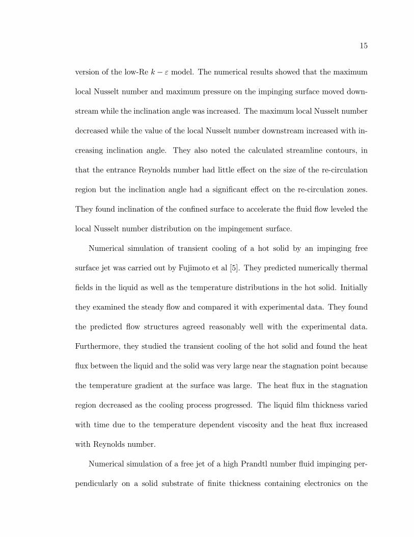
15

version of the low-Re k− ε model. The numerical results showed that the maximum

local Nusselt number and maximum pressure on the impinging surface moved down-

stream while the inclination angle was increased. The maximum local Nusselt number

decreased while the value of the local Nusselt number downstream increased with in-

creasing inclination angle. They also noted the calculated streamline contours, in

that the entrance Reynolds number had little effect on the size of the re-circulation

region but the inclination angle had a significant effect on the re-circulation zones.

They found inclination of the confined surface to accelerate the fluid flow leveled the

local Nusselt number distribution on the impingement surface.

Numerical simulation of transient cooling of a hot solid by an impinging free

surface jet was carried out by Fujimoto et al [5]. They predicted numerically thermal

fields in the liquid as well as the temperature distributions in the hot solid. Initially

they examined the steady flow and compared it with experimental data. They found

the predicted flow structures agreed reasonably well with the experimental data.

Furthermore, they studied the transient cooling of the hot solid and found the heat

flux between the liquid and the solid was very large near the stagnation point because

the temperature gradient at the surface was large. The heat flux in the stagnation

region decreased as the cooling process progressed. The liquid film thickness varied

with time due to the temperature dependent viscosity and the heat flux increased

with Reynolds number.

Numerical simulation of a free jet of a high Prandtl number fluid impinging per-

pendicularly on a solid substrate of finite thickness containing electronics on the

16

opposite surface was carried out by Rahman et al [6]. They developed numerical

model considering both solid and fluid regions and solved it as a conjugate problem.

They investigated the influence of different operating parameters such as jet veloc-

ity, heat flux, plate thickness, nozzle height, and plate material. They validated the

computed results with the available experimental data. They found that the local

Nusselt number was the maximum at the center of the disk and decreased gradually

with radius as the flow moved downstream. The average Nusselt number and the

maximum temperature in the solid varied significantly with impingement velocity,

disk thickness, and thermal conductivity of the disk material.

A study that examined jet impingement on a surface having a constant heat flux

over a limited area was carried out by Shuja et al [7]. In this study, they took air

as the impinging gas and simulated the process with a two-dimensional form of the

governing conversation equations. They introduced four turbulence models, including

standard k−ε, low-Reynolds-number k−ε, and two Reynolds stress models to account

for the turbulence. They compared the predicted flow properties with the previously

experimental data and found that the RSTM model predictions of the flow field

close to the surface agreed better with the experimental findings as compared to the

standard k−ε and low-Re k−ε models. However, they obtained similar temperature

fields from RSTM and low-Re k − ε.

Numerical simulation of three-dimensional laser heating of steel substrate when

subjected to impinging gas was also carried out by Shuja et al [8] They considered

the gas jet impinged onto the workpiece surface co-axially with the laser beam. They

17

tested the k − ε model with and without corrections and the Reynolds stress model

under conditions of constant heat flux introduced from the solid wall. They selected

the low-Re- k−ε model to account for the turbulence whereas they used the transient

Fourier heat conduction equation to compute the temperature profiles in the solid

substrate. They extended their study to include four gas jet velocities, and they

found that the impinging gas jet velocity had a considerable effect on the resulting gas

side temperature. Moreover, the temperature at the surface decreased rapidly as the

radial distance from the heated spot center increased. In addition, the temperature

profiles inside the solid substrate were not influenced considerably by the assisting

gas jet velocity.

Impinging jet studies for turbulence model assessment were carried out by Craft

et al [9]. They applied four turbulence models to the numerical prediction of turbulent

impinging jets discharged from a circular pipe measured by Cooper et al [10]. These

included one k − ε eddy viscosity model and three second-moment Reynolds stress

closure models. The numerical predictions indicated that the k− ε model and one of

the Reynolds stress models led to far too large levels of turbulence near the stagnation

point. This excessive energy in turn induced much too high heat transfer coefficients

and turbulent mixing with the ambient fluid. The other two second-moment closure

models, adopting new schemes for accounting for the wall’s effect on pressure fluctu-

ations, did much better; though one of them was clearly superior in accounting for

the effects of the height of the jet discharged above the plate. However, none of the

schemes was entirely successful in predicting the effects of Reynolds number. They

18

suggested the main cause of the failure was the two-equation eddy viscosity scheme

adopted in all cases to span the near-wall sub-layer rather than the outer layer models

on which their study was focused.

The cooling of a heated pedestal mounted on a flat plate was numerically sim-

ulated by Parneix et al [11]. They adopted normal velocity relaxation turbulence

model (V2F model) in an axisymmetric geometry and they obtained results for a

range of Reynolds numbers and jet-to-pedestal distances. They showed that the local

heat transfer coefficient exhibited a minimum in the stagnation region, which was

rather different from the behavior of an impinging jet on a flat plat. They concluded

that complex features like separation and re-attachment on the plate strongly influ-

enced the wall temperature distribution and heat transfer. For comparison, they also

obtained results with the widely used k − ε turbulence model and found that the

agreement with the data was poor.

An experimental study of flow field of an axisymmetric, confined and submerged

turbulent jet impinging normally on a flat plate was carried out by Fitzgerald and

Garimella [12, 13] using Laser-Doppler Velocimetry. Experiments were conducted

with two different nozzle diameters, with a range of nozzle-to-target spacing and with

a range of Reynolds number. They mapped the toroidal re-circulation pattern in the

out flow region, characteristic of confined jets, and presented velocities and turbulence

levels over a fine measurement grid in the pre-impingement and wall-jet regions.

Studies on vortex structure and heat transfer in the stagnation region of an im-

pinging plane jet were conducted by Sakakibara et al [14]. They measured velocity

19

and temperature field in the stagnation region of an impinging jet simultaneously

by digital particle image velocimetry and laser-induced fluorescence. They observed

counter-rotating vortex pairs in the stagnation region which swept cold fluid toward

the wall and ejected high-temperature fluid toward the outer region. The weighed

probability distribution function (pdf) of the turbulent heat flux indicated that the

contribution of this ejection mechanism to the net heat flux was dominant. The

stream-wise vortex pair was transported from the free-jet region to the stagnation

region, and the vorticity was amplified by the main stream of what in the vicinity of

the wall.

An experimental study was carried by Chung et al [15] to investigate the flow and

heat transfer characteristics by jets impinging upon the rib-roughened convex surface.

They found similar Nusselt number distributions for both smooth and roughened sur-

faces. However, after the first rib position, the Nusselt numbers on the rib-roughened

surface were higher than Nusselt number on the smooth surface. They found heat

transfer rate increased due to flow separation and re-attachment for pitch to height

ratio of the rib greater or equal to 10. Beyond the region corresponding to the ratio

of stream-wise distance from the stagnation point to the pipe nozzle diameter, the

rib roughness did not affect the heat transfer.

2.1.2 Free Jets

The fully developed flow field farther away from the tube exit is well described by

the Schlichting’s similarity solution [16]. However, the similarity assumption failed

20

to hold in the developing region of the jet close to the exit. Analytical solutions for

the developing jet from a fully developed laminar tube flow were conducted by Lee et

al [17]. Their work proposed two approximate methods to analytically calculate the

developing jet velocity field from a fully developed laminar (parabolic) axisymmetric

tube flow.

Three-dimensional turbulent jets with rectangular cross-section were simulated

numerically by Wilson and Demuren [18]. They performed computations for different

inlet conditions, which represented different types of jet forcing within the shear

layer. They observed the phenomenon of axis-switching in some cases; and at low

Reynolds numbers, it was based on self-induction of the vorticity field, whereas at

higher Reynolds numbers, the turbulent structure became the dominated mechanism

in natural jets. Budgets of the mean stream-wise velocity showed that convection was

balanced by gradients of the Reynolds stresses and the pressure.

A pdf (Probability Density Function) approach to explain the turbulent axisym-

metric free jet flow was adopted by Chen and Hong [19]. Their computational results

revealed that the pdf approach gave consistency in the higher-order moments and

radial budget of third moments of velocity, and that the neglect of the mean-strain

production, the rapid part of the pressure correction and the dissipation were respon-

sible for deviations between moment-closure models and experiments. Hence, the pdf

models appeared to be more suitable than conventional moment-closure models in

terms of revealing turbulence structure.

Numerical predictions of mean and turbulent characteristics of the axisymmetric

21

vertical jet (momentum-dominated) and plume (buoyancy-dominated) were reported

by Pereira and Rocha [20]. They used an algebraic stress and flux model to close

the time-averaged Navier-Stokes and energy equations and gave special attention

to the numerical model, which was based on a finite-volume discretization of the

elliptic form of flow equations. They used special procedure to treat free boundaries

and to compute the flow up to the similarity regime. Their results showed that

the essential characteristics of the flows, especially for the plumes, were correctly

reproduced. However, some discrepancies arose from the comparison of predicted

and experimental results.

A numerical study was performed by Riopelle et al [21] to determine the influence

of weak ambient motion and of the associated pressure field on the flows of free plane

vertical turbulent jets and plumes. A nested grid control volume technique with

buoyancy-extended k − ε model plane was used to model turbulent jets and plumes

issuing into open spaces as well as into two-dimensional rooms of various sizes. The

results indicated that slight variations in the ambient pressure distribution affected

jet and plume development and similarity relationships.

Near-wall modeling of plane turbulent wall jets was done by Gerodimos and So

[22]. After its failure to predict the jet spreading correctly, they investigated the

appropriateness of two-equation modeling; particularly the importance of near-wall

modeling and the validity of the equilibrium turbulence assumption. They analyzed

an improved near-wall model and three others, and compared predictions of these

with measurements of plane wall jets. They calculated the jet spread correctly by the

22

improved model, which was able to replicate the mixing behavior between the outer

jet-like and inner wall layer and was asymptotically consistent. They obtained good

agreement with other measured quantities. However, other near-wall models tested

were incorrect to predict the jet spread.

Numerical simulation of turbulent jet flow and combustion was carried out by

Zhou et al [23]. Their work applied k − ε turbulent model, with pressure boundary

condition for the entrainment atmosphere surface, to calculate the steady free jet flow.

Based on the fulfillment of the above isothermal jet flow, they simulated combusting

jet flows of diffusion flame and partial premixed-flame using the assumption of fast

chemical reaction and Eddy-Dissipation Concept (EDC) model, respectively. They

compared their numerical results with the experimental and theoretical results. Their

numerical results of isothermal jet and diffusion jet flame agreed well with tests by

Panchapahesan and Lumley [24], and Lockwood and Moneib [25]. They found that

EDC model had some errors in modeling partial premixed jet flames.

Numerical simulations of two-dimensional laminar methane/air premixed jet flames

with a detailed chemical kinetics mechanism were also conducted by Zhou et al [26].

The focal point of the work was to demonstrate the sensitivity of the modeling of the

detailed chemical kinetics on the flame temperature and concentrations of major com-

ponents for three different equivalence ratios. They found the temperature and major

species distributions were in good agreement with the experimental measurements by

Nguyen et al. [27], but some radical species profiles still deviated from experiments.

They obtained the typical flame structure of the steady jet.

23

Numerical modeling of turbulent jet diffusion H2/air flame with detailed chem-

istry was carried out by Zhou et al [28]. Their focus was on the investigation of an

axisymmetric turbulent hydrogen/air diffusion flame using a time-dependent numer-

ical model with a detailed chemical mechanism. They used an algebraic correlation

closure (ACC) model to couple turbulence and chemistry. They found temperature

and major species distributions were in good agreement with experimental measure-

ments. They showed that the numerical results obtained from the detailed chemistry

calculations depended on how the turbulent diffusion coefficients were selected for

species and energy equations.

Studies on transient turbulent gaseous fuel jets for diesel engines were carried out

by Hill and Ouellette [29]. They determined the conditions under which transient

turbulent jets were self-similar, quantified the appropriate similarity parameter and

tested the assumption of self-similarity even with under expansion and with jet in-

jection near a boundary wall. They used the idea of Turner [30] that the transient

turbulent jet could be modeled as a steady jet headed by a spherical vortex to evalu-

ate the constant of proportionality used to establish the direct relationship between

the jet penetration distance well downstream of the virtual origin with the square

root of the time and the fourth root of the ratio of nozzle exit momentum flow rate

to chamber density. Using incompressible transient jet observations to determine the

asymptotically constant ratio of maximum jet width to penetration distance, and

the steady jet entrainment results of Ricou and Spalding [31], they established the

penetration constant. They showed this constant was also true for compressible flows

24

with substantial thermal and species diffusion, and even with transient jets from

highly under-expanded nozzles. They made observations of transient jet injection in

a chamber in which, as in diesel engine chambers with gaseous fuel injection, they

directed the jet at a small angle to one wall of the chamber. In those tests with under-

expanded nozzles they found that at high nozzle pressure ratios, depending on the

jet injection angle, the jet penetration could be consistent with the established pene-

tration constant. At low-pressure ratios the presence of the wall noticeably retarded

the penetration of the jet.

Turbulent transient gas injections were also studied by Ouellette and Hill [32].

They used multi-dimensional simulations to analyze the penetration, mixing, and

combustion of such gaseous jets. They evaluated the capability of multi-dimensional

numerical simulations based on k − ε turbulence model to reproduce the experi-

mentally verified penetration rate of free transient jets. Their model was found to

reproduce the penetration rate dependencies on momentum, time, and density but

was more accurate when they modified one of the k − ε coefficients. They used the

simulation to determine the impact of chamber turbulence, injection duration, and

wall contact on transient jet penetration. They showed gaseous jets and evaporating

diesel sprays with small droplet size mixed at much the same rate when injected with

equivalent momentum injection rate.

Entrainment characteristics of transient gas jets were proposed by Abraham [33].

He presented results of theoretical analysis and computation of transient gas jets

in a quiescent ambient environment, with injected to three ambient density ratios.

25

He used k − ε model for turbulence and showed that the entrainment rate varied

linearly with axial penetration and the total mass entrained had cubic dependence on

axial penetration of the gas jet. He found that the actual values of these quantities

depended on a constant whose value obtained from measurements and quoted in the

literature varied by as much as a factor of 2.

A numerical scheme for the transient simulation of incompressible turbulent con-

fined jet flow of variable density was developed by Singh et al [34]. Their scheme was

capable of capturing the essential flow features of confined jet flows and it predicted

the level of ambient fluid entrainment fairly accurately. They found that aspect ra-

tio and density ratio were the main factors that influenced entrainment and mixing.

These factors were also responsible for causing jet instability and re-circulation within

the mixing tube. They showed that Reynolds number had a negligible effect over the

entrainment ratio. Moreover, as the jet moved away from the tube inlet, the level of

entrainment increased for short distances and vice-versa. On the other hand, mixing

between the jet and the entrained fluid improved if they moved the jet away from the

tube inlet.

The turbulent exponential jet was studied by Breidenthal [35]. He postulated a

new self-similar flow when nozzle exit velocity employed was exponentially increasing

in time. He argued that the acceleration of the jet would imply a lower entrainment

rate.

The jet characteristics of CNG injector with MPI system were studied by Boyan

et al [36]. They developed a theoretical model that assumed the natural gas transient

26

jet could be characterized as a spherical vortex interacting with a steady jet. They

employed Schlieren photographs that revealed a low-pressure gas jet’s starting and

extending process from the nozzle. They compared the model with the experimental

results for the tip penetration of round jet and found the results had similar charac-

teristics. The results showed that the tip penetration was proportional to the square

root of time. Moreover, the tip penetration of the gas jet was longer than that of

gasoline provided that the per unit time calorific values of the injecting fuel were the

same.

Experimental investigations of the development of transient jets and evolving jet

diffusion flames were carried out by Park and Shin [37] using a high-speed Schlieren

photography. They measured the jet tip penetration velocities and normalized jet

widths of the primary vortex. They showed that the development behavior in the

presence of a flame was greatly different from that in a transient jet. The discernible

differences were the delay of the roll-up of the primary vortex, the faster spreading

after the roll-up due to the exothermic expansion, and the survival of only a primary

vortex. They reported that the jet tip penetration velocity varied with downstream

distance and an increase in Reynolds number gave rise to a higher tip penetration

velocity.

The velocity field of fully pulsed air jets (no mass flow in between pulses) was

studied experimentally in detail by Bremhorst and Hollis [38]. They found the en-

trainment in fully pulsed air jets was much higher than the steady or partially pulsed

jets. Even though the jet spreading and volumetric entrainment were increased in

27

these pulsatile jet flows, the basic structure of the jet did not change. The velocity

profiles were self-similar; the spreading rate was linear with the downstream distance;

and most importantly, the entrainment scaled with the square root of the aggre-

gate jet momentum flux. The results were consistent, except for the proportionality

constants, with Taylor’s entrainment hypothesis [39].

Experimental investigation of unsteady submerged axisymmetric jets was carried

out by Fang and Sill [40]. They measured the centerline velocities of linearly accelerat-

ing turbulent jets. The results of the experiment indicated that significant deviations

(lower normalized velocities) from the steady case existed in the linearly accelerating

jets. These aberrations were observed even in the far field. This was interesting since

the majority of the pulsed jets were effective only in the near field. However, in this

study of unsteady jets carried out by Fang and Sill [40], neither the spreading rates

nor the entrainment rates were reported for these monotonically changing unsteady

jets.

Kouros et al [41] measured the spreading rate of an unsteady turbulent jet. They

reported the penetration length and spreading rate of a non-harmonic unsteady jet.

They found the visible spreading rate of an unsteady jet produced by their experi-

mental set up was less than half of the steady jet value.

The experimental investigation of round, incompressible, impulsively started tur-

bulent jets was carried out by Johari et al [42].They found that the flow was comprised

of a starting vortex that separated from the rest of the jet in the near field. The start-

ing vortex and the flow immediately behind it were in unsteady motion. They found

28

the penetration of the jet tip scaled with the square root of time, normalized by

the nozzle diameter and velocity, and the celerity of the jet tip was approximately

one-half of the centerline velocity of a steady jet, with the same nozzle exit velocity,

at the same location. Results of chemically reactive experiments indicated that the

fluid in the vicinity of the jet tip mixed with the ambient fluid faster than the rest

of the jet. Their findings revealed that the extent of the region near the jet tip with

improved mixing became larger as the jet traveled further downstream. They found

the more rapid mass mixing at the jet tip implied faster momentum diffusion, which

corroborated the slowing down of the jet tip in comparison of the steady jet.

Detailed measurements of the centerline-mixing behavior in the near field of

variable-density jets were performed by Papadopoulos and Pitts [43]. They made

real-time measurements of jet fluid concentration for a propane jet and a methane

jet issuing into still air utilizing Rayleigh light scattering. They used fully developed

turbulent conditions as initial conditions and made testing for flow rates yielding

Reynolds numbers in the range 3.3 × 103 − 2.3 × 104, based on average discharge

velocity, exit diameter and initial fluid properties. They found that the centerline

decay characteristics in the near field exhibited a downstream shift with increasing

Reynolds number, which was attributed to the initial velocity distribution at the jet

exit. The investigation of the mean and turbulent characteristics of the initial veloc-

ity distribution yielded a proposed near-field scale variable that effectively captured

this dependence on Reynolds number. They achieved the collapse of the near-field

centerline velocity and concentration distribution using the proposed scaling. More-

29

over, they extended their analysis for a constant density jet to the intermediate and

self-similar far fields further downstream using a dynamic length scale based on the

local centerline turbulent intensity [44]. The normalized mean velocity distributions

of an air jet collapsed over the entire flow distance investigated when they normalized

the axial distance by the proposed length scale, thus scaling the virtual origin shift

and effectively incorporating the Reynolds number dependence.

Mi and Nathan [45] experimentally investigated the effect of small vortex-generators

(tabs) placed at the exit plane of an axisymmetric smooth contraction on scalar mix-

ing in the developing region of a turbulent jet. They showed that the presence of tabs

profoundly distorted the jet flow field and consequently modified the scalar mixing

characteristics significantly. They found that tabs caused the mean temperature to

decrease more rapidly with the downstream distance, implying an increased mixing

rate. Furthermore, they found that two tabs distorted the jet from axisymmetric

state more dramatically than four tabs.

Natural coherent structures in the near field of an axisymmetric jet was educed

and their dynamics studied experimentally by Aydore and Disimile [46] using hot-wire

anemometry. They positioned the jet, originating from a fully developed turbulent

pipe flow, four jet diameters upstream from an impingement plate. Based on the

pipe diameter, they maintained a jet Reynolds number of 1.3 × 104. Using the life

cycle method for coherent structure eduction, they obtained phased-averaged vortic-

ity contours in the jet near field, within 2.3 diameters of the pipe exit. Vorticity

contours suggested that large coherent structures existed in the middle of the shear

30

layer at approximately one jet diameter downstream from the pipe exit. Their size

was the maximum at this location. A decay region was also observed 1.6 diameters

downstream from the pipe exit. Moreover, they evaluated individual terms in the

coherent vorticity equation and examined significant terms.

Turbulent flow and heat transfer characteristics of a two-dimensional oblique wall

attaching offset jet (a two-dimensional slot jet issued into quiescent surroundings

above an inclined plate) were experimentally investigated by Song et al [47]. They

measured the local Nusselt number using liquid crystal as a temperature sensor,

the jet men velocity, turbulent intensity and wall static pressure coefficient profiles.

They observed that the time-averaged re-attachment point nearly coincided with the

maximum Nusselt number point for all oblique angles, but the maximum pressure

point did only for zero inclination. They found the decay of the maximum jet velocity

in the stream-wise direction obeyed the conventional −1/2 power law of the wall

attaching offset jet for the inclination angle (oblique angle) less than or equal to

30◦. They well correlated the re-attachment length and maximum pressure point

with offset ratio (height of the jet/diameter of the jet) and oblique angle. They

presented correlations between the maximum Nusselt number and Reynolds number

for all oblique angles tested.

2.1.3 Opposing Jets

Hosseinalipour and Mujumdar [48, 49] dealt with the numerical simulation of

the flow, mixing, and thermal characteristics of a symmetric steady laminar two-

31

dimensional confined opposing jet configuration for the case when the two jets were

equal and unequal. They presented results for two boundary conditions; constant

wall temperature and insulated walls. They made an extensive parametric study to

investigate the effects of geometric, hydrodynamic, and thermal parameters on the

flow and heat transfer characteristics of such systems. They showed that mixing of

two oppositely directed confined jets caused major hydrodynamic distortions, which

persisted in the merged flow in the exit channel. The results for three different con-

figurations showed that the decaying disturbances and the flow re-development that

occurred affected significantly the heat transfer in the exit channel. Their findings

showed that unequal jet configuration with different width jets caused more distortion

in the flow field compared to equal jet and unequal jet with equal jet width config-

urations. They found these distortions affected the Nusselt number distribution on

both top and bottom more than those for the equal jet and unequal jet with equal

jet width.

Johnson [50] examined impingement of laminar fluid jets in a confined cylindrical

chamber using flow visualization, Laser Doppler Anemometry (LDA) measurements

and steady and unsteady three-dimensional finite volume numerical simulations using

boundary fitted non-orthogonal coordinates. He presented results that dealt with

the cases of flow imbalance issuing from the nozzles. His measurements and flow

visualization of unequal flow cases with ∼3:1 flow rate ratios in an opposed two

jet configuration indicated an asymmetric flow field with significant downward re-

circulation from the region away from the nozzles to the nozzle region and a jet-to-jet

32

impingement point very close to the low flow rate nozzle. Steady and unsteady

numerical simulations he made confirmed the asymmetry of the flow field at these

conditions and he found reasonable agreement for the jet-to-jet impingement point.

He showed large areas of re-circulation in the mix chamber would lead to poor mixing

due to the possibility of unmixed fluid leaving the chamber and the increase in the

residence time of the mixing fluids. Subsequent to the above study, the author’s

results herein [51] dealt with modifying an existing flow imbalance and suggested

alternative momentum arrangements to improve the flow characteristics.

Hosseinalipour and Mujumdar [52] investigated numerically to predict and to

compare the fluid flow and heat transfer characteristics of two-dimensional turbulent

confined and opposing jet flows. They used five low-Reynolds-number k − ε models

and the standard high-Reynolds-number model. They also tested the newly proposed

Yap correction with low-Reynolds-number models in order to investigate its effect on

the heat transfer predictions for the impinging jet case. They found that in some

models this correction improved the heat transfer predictions. They compared the

simulation results with the available data for fluid flow and heat transfer for a single

slot jet impingement on a flat plate. They presented only numerical results for the

opposing jet case due to lack of experimental data. They performed a parametric

study for flow and heat transfer characteristics in the opposing jet configuration.

Heat transfer between two opposed, non-isothermal jets under corotation was

investigated numerically by Sheu and Liou [53]. They analyzed the efficiencies of

heat transfer between two jets under various system conditions. They also included

33

the problem in the limit of zero rotating speed on one side in their work. They

found a critical rotating speed in this limit at which the efficiency of heat transfer

was minimum. They made a comparison of efficiencies of heat transfer among typical

cases. Furthermore, they interpreted relevant results physically.

Lam and Chan [54] investigated the penetration and spreading of a round jet into

an ambient counter-flow using the planer laser-induced fluorescence (LIF) technique.

The LIF images enabled them to obtain the instantaneous concentration field of the

penetrating jet effluent. They observed large-scale wandering of jet penetration, which

led to significant temporal and spatial fluctuations in the location of the dividing

interface between jet effluent and ambient fluid. They found that the penetration

distance and the lateral spreading width of the jet exhibited fluctuations with covering

ranges as large as their corresponding time-averaged values. They found the degree

of fluctuations in these penetration and spreading parameters increased with the jet-

to-current velocity ratio, but essentially scaled with the mean penetration distance.

They also attempted to predict the mean penetration distance by considering the

decay of centerline jet velocity under a hypothesis that the counter-flow affected the

jet via a simple compression of the axial coordinates of the jet flow.

A two impinging jet mixer for precipitation process was investigated by means

of the laser induced fluorescent technique by Benet et al [55]. They used neutral-

ization reactions with a fluorescent PH-indicator to reveal the mixing process up to

the molecular level. They derived a phenomenological mixing model on the basis

of experimental results. The mixing model involved a macro-dilution process and a

34

coalescence-redispersion process through which the fluids were contacted at the molec-

ular level. They applied the mixing model to the precipitation of barium sulfate and

found predictions were very close to experimental results.

Witze and Dwyer [56] used a hot-film anemometer to investigate the mean ve-

locity and turbulence intensity distributions in turbulent radial jets. They showed a

geometric parameter termed as the constrained ratio (nozzle diameter to separation

distance) to characterize radial-jet behavior. They defined constrained radial jet as

one for which the nozzle walls constrained the flow leaving the orifice to be parallel

if the constraint ratio was large. They also defined a small constraint ratio which

was representative of two opposing free axisymmetric jets, the collision of which pro-

duced an impinged radial jet. They found that the well-behaved constraint radial jet

spread at the same rate as did the familiar plane jet, whereas the impinged radial

jet spread at a rate more than three times as fast. They demonstrated that neither

type of radial jet was amenable to a self-similar analytic solution and they showed

the impinged radial jet required numerical solution technique. They demonstrated

an empirical solution for the constrained radial jet.

An experimental investigation of a conical flow formed by the interaction of two

asymmetric turbulent curved wall jets past a circular cone was presented by Jarrah

et al [57]. They made measurements of velocity and turbulence intensity profiles of

the two jets in the wall jet, the interaction, and the merged jet regions. They found

the location of the interaction region of the two opposing curved wall jets and flow

direction of the merged jet depended primarily on the ratio of the slot exit velocities

35

of the two jets. The mean velocity and stream-wise turbulence intensity profiles of

the merged jet were similar to those in a turbulent free jet. Self-similar mean velocity

profiles for different values of downstream location prevailed up to the beginning of the

interaction region, regardless of jet exit velocity ratios. They showed that stream-wise

and lateral turbulence intensities increased with increasing the stream-wise distance

up to the interaction region, where the turbulence behavior became random and

was characterized by larger peak values of the turbulence intensity compared to the

wall jet region. Moreover, they showed that the maximum velocity decay and jet

half-width growth increased parabolically with stream-wise distance and observed no

significant effect of the conical shape. They carried out flow visualization for several

exit jet velocity ratios and saw three-dimensionality to be reduced as the secondary

jet momentum increased.

2.1.4 Non-Conduction Limited Laser Heating

Gonsalves and Duley [58] presented the results of a quantitative investigation into

the interdependence of the parameters, the incident power, the radius of the focused

spot on the target, the cutting speed, the cut width and the sheet thickness. They

also showed how these results could be generalized to provide a prediction of the

power required to achieve a certain cutting velocity or cut width with predetermined

focal area on thin sheets of arbitrary composition.

Modest and Abakians [59] considered partial vaporization of a semi-infinite medium

caused by a moving Gausian laser irradiation (across the vaporization surface). They

36

used a simple integral method for the evaluation of temperature distribution, assum-

ing relatively minor thermal losses due to convection, conduction and radiation. They

solved the relevant non-linear partial differential equation numerically and presented

the results for the groove depth, width and shape for variety of laser and solid pa-

rameters. Their results clearly indicated that surface heat losses were nearly always

negligible. It was seen that, for a Gaussian beam, the bottom of the groove might

have a sharp apex. The model was also able to predict quantitatively groove depths

accurately for a few situations.

Bang and Modest [60] analyzed numerically multiple reflection and beam guid-

ing effects during laser machining. They considered that the surface of the treated

material reflected the laser irradiation in a fully diffuse fashion, limiting the analysis

to bodies that had a rough surface during laser evaporation (e.g. micro-explosive re-

moval, violent surface boiling). For local irradiation calculations the material surface

was divided into a number of triangular elements with liner interpolation functions.

The net radiative flux for these elements was obtained from standard view factor

theory. The irradiation calculations were combined with a simple integral method

governing conduction losses into the medium, and the resulting groove shape and

depth were found through an iterative procedure. They concluded that beam guid-

ing played an important role in forming the fully developed groove, resulting in an

increased effective absorptivity. Due to channeling from the upstream wall as well

as the side walls, the evaporation zone extended farther down-stream and the fully

developed groove cross-sections had steeper groove walls with a flatter center region

37

as compared to that predicted by the previous model without reflection effects. For

materials with relatively large reflectivity, the material removal rate was increased

significantly, resulting in an increased effective absorptivity. Generally, the beam

guiding effects became significant for high reflectivity materials and/or deep groove

cases. The groove depth could be increased by using lenses with larger focal lengths

focused slightly inside the material. Larger focal length lenses had larger minimum

beam radii at the focal plane, but with a lower beam divergence focused near the

surface. On the other hand, flatter grooves with steeper walls could be obtained by

using lenses with shorter focal lengths.

Roy and Modest [61] developed a three dimensional conduction model to predict

the temperature distribution inside the solid and the shape of a groove formed by

partial evaporation of a semi-infinite body using a moving CW laser with a Gausian

beam profile. This had application in laser machining where material was removed

by repeated scanning of a focused beam on the work piece surface. They solved

the governing equation using a finite difference method on an algebraically generated

boundary-fitted coordinate system. They presented the groove shape and tempera-

ture distribution in the solid for both constant properties and variable properties, for

different speeds, for various laser power levels and for different beam profiles. The

groove shapes for constant thermal properties were compared with three-dimensional

boundary element conduction model solution and a quasi-one-dimensional conduc-

tion model solution, in which the conduction losses were approximated using a simple

integral method. Their model compared well with the three-dimensional boundary

38

element model for all ranges of laser parameters, and, when thermal losses due to

conduction were minor, the one-dimensional results were also in good agreement with

the three-dimensional boundary element predictions. They concluded that heat loss

by conduction could be between 25 to 45% of absorbed laser power, at higher power

losses were lower. They obtained experimental results for material removal rates

and groove shapes on silicon nitride, which were found to agree well with theoretical

predictions for shallow grooves.

Bang et al [62] analyzed theoretically the beam guiding effects during laser ma-

chining for ceramics due to multiple reflections in the groove for two extreme cases–

-purely specular and purely diffuse reflections. Specular reflections were valid for

materials that had a smooth surface during laser evaporation (small optical rough-

ness as compared to the laser wavelength). For such cases the material surface was

divided into a number of rectangular patches using a bicubic surface representation

method. The net radiative flux for these patch elements was obtained by ray trac-

ing methods. The resulting radiative flux due to specular reflections was combined

with the three dimensional conduction equation governing conduction losses into the

medium, and the resulting groove shape and depth were found through an iterative

procedure. Diffuse reflections were valid for materials that had a very rough sur-

face during material removal. To address beam coupling due to diffuse reflections,

irradiation calculations employing view factor were combined with three-dimensional

calculation model. Considering multiple reflections resulted in an increased absorp-

tivity and deeper grooves, accompanied by a flatter profile near the centerline and

39

steeper slopes in the other parts of the groove cross-section. They predicted for the

tested set of parameters, material removal rates were increased up to 40% by specular

reflections and up to 70% by diffuse reflections. They compared their results with

experiments, hot-pressed silicon nitride ceramic showed increased beam coupling for

deeper grooves (high power and/or slow scanning speeds) as predicted by considering

multiple reflections. The agreement between theoretical calculations and experimen-

tal data for material removal rate and groove shape was good, if multiple reflections

were assumed to be diffuse.

Modest [63] developed a three-dimensional conduction model to predict the tran-

sient temperature distribution inside a thick solid that was irradiated by a moving

laser source, and the changing shape of a groove carved into it by evaporation of

material. The laser might operate in CW or in pulsed mode with arbitrary tempo-

ral as well as spatial intensity distribution. He solved the governing equations using

a finite-difference method on an algebraically generated boundary-fitted coordinate

system. He verified this transient model with three-dimensional codes that were

limited to quasi-steady CW operation. He presented the groove shapes and tem-

perature distribution, as well as their transient development, for various machining

conditions, demonstrating the differences in the ablation process between CW, pulsed

and Q-switched (or other pulses of extremely short duration) laser operation. The

results showed that during short-pulsed laser ablation conduction losses were essen-

tially negligible, resulting in substantially larger removal rates than for CW operation.

Ablation with normally pulsed lasers, on the other hand, resulted in removal rates,

40

which approached those of a Q-switched laser, but the thickness of the heat-affected

layer was much larger, approaching that of the CW laser. The calculation further

indicated that, during short-pulsed laser ablation, the material cooled off rapidly after

the end of the pulse, returning to ambient conditions well before the beginning of the

subsequent pulse.

Modest [64] developed a model of full three-dimensional transient through-cutting

in thin sheets. He also developed a two-dimensional axisymmetric version to model

and predict results for drilling. He solved three-dimensional conduction equation

numerically using boundary-fitted coordinates. Using his model he found that under

all circumstances even the maximum possible convection and radiation losses could

have only a negligible effect on temperature and groove development.

Yilbas and Yilbas [65] studied the interaction mechanism of vapor generated by

laser beam over the surface of work piece. The vapor heated the work piece surface and

absorbed some fraction of incident energy. They developed a computer program to

model gas dynamic equations in one-dimension with additional terms for absorption of

laser beam, radiation losses and conduction. They assumed that vapor was comprised

of heavy particles and free electrons, each species behaving as a perfect gas. They

found that the evaluation of the expansion of vapor plug was sensitive to variations in

initial conditions. The vapor temperature increased from initial value to 10000 K in

10−7–10−6 sec after which further increment occurred relatively slowly. The leading

edge of the vapor had velocity of the order of 4000-7000 m/s.

Yilbas et al [66] examined the absorption of a laser beam at different wavelengths

41

by a partially ionized vapor during the interaction mechanism. They distinguished

the interaction of the high and low power laser beam with plasma. They showed that

different metal vapors at similar temperatures and densities had absorption depths,

which might differ by an order of magnitude. They also showed that the free electron

temperature became significantly different from the heavy particle temperature for

power intensities above critical level which was typically greater than 1014 W/m2.

Wei and Ho [67] determined energy transfers and penetration velocity during a

high-energy drilling or welding process. The beam energy of a Gaussian distribution

incident on the free surface of a liquid layer that separated unmelted solid and vapor

was balanced with the heat conduction and latent heats for melting and evaporation.

They examined the effects of the beam power and the energy distribution on the high

energy beam drilling. The normal pressure condition at the vapor-liquid interface

was used to determine the shape of the vapor-liquid interface. The heat conduction

in both the axial and radial directions, heat of evaporation and melting were taken

into account. The fusion line, however, was calculated by using the enthalpy method.

They developed a quasi-steady, axisymmetric heat conduction model to investigate

the penetrating process of the cavity produced by high energy beam. The shape of

the fusion zone and the penetration velocity were determined as a function of energy

distribution parameters and the beam power, rather than specified a priori. They

showed that the energy distribution parameter had stronger effects than the beam

power on the high-energy beam drilling or welding process. The penetration velocity

increased with increasing beam power or decreasing energy distribution parameter.

42

Increasing the energy flux resulted in a slight increase in radial conduction loss. Since

the sensible heat of raising the liquid from the melting temperature to the base

temperature was small, the energy transferred to the liquid-solid interface became

larger for a higher energy flux. This resulted in a non-linear and significant increase

in the penetration velocity at a high beam power or a small energy distribution

parameter. High temperature occurred near the cavity base.

Ganesh et al [68,69] developed a comprehensive model to study the laser drilling

process and used volume of flow technique to track the position of moving vapor front

and recession of surface.

Zhang and Faghri [70] investigated the melting and vaporization phenomena dur-

ing the laser drilling process. The locations of the solid-liquid and liquid-vapor in-

terfaces were obtained by solving energy conservation equations at interfaces. The

dependence of saturation temperature on the back pressure was taken into account

by using the Clausius/Clapeyron equation. They also included the conduction heat

loss to the work piece and solved it using an integral approximation method. The

predicted material removal rate agreed well with the experimental data. The amount

of heat loss through conduction was found to be very small and its effect on the

vaporization was not significant. However, the location of melting front was signifi-

cantly affected by conduction heat loss especially for lower laser intensity and longer

pulse. The existence of sub-cooling in the solid was helpful in reducing the thickness

of recast layer.

A two-step gas-dynamic model of laser ablation in an ambient gas atmosphere

43

was proposed by Gusarov et al [71]. The initial one dimensional stage was related

to obtain plume formation and described heating, melting and evaporation of the

target, the target-vapor interaction in the boundary layer, and vapor dynamics. The

final two-dimensional stage was responsible for the formation of energy and angular

distributions of the ablated material. Interaction between the vapor and ambient

gas was taken into account by two-component gas-dynamic equations. Numerical

analysis of laser ablation in ambient gas atmosphere and the analysis revealed that

both kinetic energy of ablated atoms and width of their angular distribution deceased

with ambient pressure. They compared the dynamics of ablated material expansion

and its energy distribution with the experiment.

Kar et al [72] developed a simple mathematical model for the cutting of thick-

section stainless steel using a high power chemical oxygen iodine laser. The model was

based on an overall energy balance, and it related the cutting depth with various pro-

cess parameters that could be used to predictively scale the laser materials processing

performance to very thick sections. They examined the effects of absorptivity and the

velocity of the cutting gas jet on the kerf depth and width. The study indicated that

thick metal cutting performance might be improved by producing narrow kerf widths.

The scaling law for cut depth per unit power closely agreed with the experimental

data at low cutting speeds since it was obtained by assuming a large conduction heat

loss that held good at low cutting speeds. The laser-plume interaction and effective

absorptivity played an important role in the cutting performance of a laser beam.

Semak and Matsunawa [73] carried out a theoretical analysis of the energy balance

44

in the laser-metal interaction zone. They considered the heat transfer due to the

recoil-pressure-induced melt flow. The results of numerical simulations showed the

recoil pressure play a significant role in ejection of the melt from the interaction zone

even for low melt surface temperatures close to the melting point. High-velocity melt

flow was generated in the interaction zone for beam intensities typically used in laser

cutting/welding; thus, the melt-flow pattern could not be considered as the motion

of a cylinder in an infinite liquid pool. Under typical industrial cutting/welding

conditions about 70-90% of laser intensity absorbed in the beam interaction zone

was carried away from the interaction zone by the metal flow; thus, the convection-

related terms could not be ignored neither in calculations of the energy balance in

the interaction zone nor in calculations of the thermal field in the weld pool or in the

vicinity of the cutting front. The velocity of the keyhole-wall front or cutting front

was determined by the absorbed laser intensity and could be either smaller or higher

than the beam’s translation velocity.

Chapter 3

MATHEMATICAL MODELLING

3.1 Mean-Flow Equations

In the present study two cases are considered; i) a high temperature air/helium jet

and ii) a high temperature helium jet and the opposing air jet at ambient temperature

is/are entering the initially stagnant and air ambient. Consequently, a mixture of

helium and air is formed, which is denoted as He-air mixture. Moreover, the gas

mixture in the present study is considered non-reacting and the resulting flow field is

compressible, unsteady, two-dimensional, axisymmetric and turbulent. The governing

Favre-Averaged Transport Equations can be given in the following form [26,28,74]:

Continuity Equation:

∂ρ

∂t+

∂

∂xj(ρeuj) = 0 (3.1)

Species Continuity Equation:

∂

∂t(ρeYi) + ∂

∂xj(ρeuj eYi) = ∂

∂xj

(ÃρDim

∂eYi∂xj− ρu00jY

00i

!)+Ri (3.2)

Where eYi is the Favre-averaged mass fraction of the ith species (here including three45

46

species: helium (He), nitrogen (N2) and oxygen (O2) for He-air non-reacting mixture);

Dim is the diffusion coefficient of the ith species in the mixture; R is the net rate of

creation of the ith species due to chemical reaction, which is neglected here for non-

reacting gaseous mixture. The above Eq. (3.2) is not required for single species (air

jet into ambient air).

Momentum Equation:

∂

∂t(ρeui) + ∂

∂xj(ρeujeui) = − ∂p

∂xi+

∂

∂xj

£(τ ij − ρu00ju

00i )¤

(3.3)

Where τ ij is a time-averaged stress tensor and is given as:

τ ij = µ

µ∂ui∂xj

+∂uj∂xi

¶− 23µ∂uk∂xk

δij (3.4)

Energy Equation:

∂

∂t(ρE) +

∂

∂xj(ρeujH)

=∂

∂xj

"³µσ

´µ ∂eh∂xj

¶− ρu00jh00

#+

∂

∂xj

£eui ¡τ ij − ρu00i u00j

¢¤+

∂

∂xj

NsXk=1

ehk³ρDkm − µ

σ

´ ∂eYk∂xj

+

ρu00jh00µ∂ eYk

∂xj

∂eh∂xj

¶− ρu00jY

00k

+Sh (3.5)

Where Ns(= 3) is the total number of species in the gas mixture. The quantities E

and H are the total specific internal energy and total specific enthalpy of a mixture

47

which include the kinetic energy of the fluctuating turbulent field known as Turbulence

Kinetic Energy (k), i.e.,

E = ee+ 12euieui + k (3.6)

H = eh+ 12euieui + k (3.7)

Where ee and eh are the Favre-averaged specific internal energy and Favre-averagedspecific enthalpy of a mixture respectively, which are given by:

ee = cv eT (3.8)

eh = cp eT = ee+ pρ

(3.9)

Where cv and cp are the specific heat of the mixture at constant volume and constant

pressure respectively. Eq. (3.5) is valid for k ¿ eh.Sensible enthalpy for ideal gas mixture (compressible) is given as [26, 28]:

eh = NsXk=1

eYkehk (3.10)

Where ehk is the specific enthalpy of the kth species and is given as:ehk = hok + Z T

Tref.

cpkdT (3.11)

Where Tref (= 298.15 K) is the mixture reference temperature, cpk is the specific

48

heat at constant pressure for the kth species and hok is the specific enthalpy of the kth

species at Tref .

The first three terms on the right hand side of Eq. (3.5) represent energy transfer

due to conduction, viscous dissipation and species diffusion respectively. Moreover,

the last term on the right hand side of Eq. (3.5) is the time-average source term (ne-

glected in the present study for non-reacting gaseous mixture with no heat generation

due to any cause), which may be due to chemical reaction and/or any other defined

cause. In case of single species (air jet into ambient air), the species diffusion term

will be neglected. Furthermore, there is no need of Eqs. (3.10) & (3.11) in this case.

State Equation:

p = ρReT (3.12)

Where R is a gas constant.

3.2 Turbulence Equations

3.2.1 Eddy-Viscosity and Eddy-Diffusivity Concept

The term −ρu00i u00j in Eqs. (3.3) & (3.5) are Favre-Averaged-Reynolds Stresses.

It was proposed by Boussinesq that modelling these stresses may be performed by

analogy with viscous stresses in laminar flows, i.e., these stresses like viscous stresses

49

can also be put in the following form [74]:

−ρu00i u00j = µtµ∂eui∂xj

+∂euj∂xi

¶− 23

µµt

∂euk∂xk

+ ρk

¶δij (3.13)

By analogy with Favre-averaged-Reynolds stresses, −ρu00jY 00i in Eqs. (3.2) & (3.5)

and −ρu00jh00 in Eq. (3.5) are respectively the turbulent transport of ith species and

turbulent transport of enthalpy and are given in their respective order by:

−ρu00jY 00i =µtσ eYµ∂ eYi∂xj

¶(3.14)

−ρu00jh00 =µtσt

µ∂eh∂xj

¶(3.15)

Where σt, σ eY and µt are turbulent Prandtl number, turbulent Schmidt number andeddy viscosity of a mixture respectively. The ratios µt

σ eY andµtσt, by analogy with eddy

viscosity, are eddy mass diffusivity and eddy thermal diffusivity. Since turbulent

transport of momentum and scalar property (enthalpy/mass fraction) are due to

the same mechanism–eddy mixing– it is expected that the value of eddy thermal

diffusivity and eddy mass diffusivity are close to that of the eddy viscosity [75]. The

turbulent viscosity, µt, can be defined by the following relation [76]:

µt = Cµρk2/² (3.16)

50

Where Cµ is an empirical constant, k is the Turbulence Kinetic Energy and ² is the

Turbulence Dissipation Rate. These turbulence quantities may be computed by the

standard k− ² model.

3.2.2 The Standard k − ² Model

The conservation equations for the turbulence kinetic energy (k) and its dissipa-

tion rate (²) are modelled in the standard k − ² model. The modelled equation for

the Turbulence Kinetic Energy (k) is given by:

∂

∂t(ρk) +

∂

∂xj(ρeujk) = ∂

∂xj

·(µtσk)∂k

∂xj

¸+G− ρ²+ PD (3.17)

and the modelled equation for the Energy Dissipation ( ²) is given by:

∂

∂t(ρ²) +

∂

∂xj(ρeuj²) = ∂

∂xj

·(µtσ²)∂²

∂xj

¸+ C1

²

k(G+ PD)− C2ρ²

2

k(3.18)

Where G is the rate of generation of turbulence kinetic energy, ρ² is its destruction

rate and PD is the pressure-dilatation which is due to the compressibility effect. G

and PD are approximated respectively by the following relationships [74]:

G = −ρu00i u00j∂eui∂xj

(3.19)

PD = α1ρ¡−ρu00i u00j¢µ∂eui

∂xj

¶Mt + α2ρ²M

2t (3.20)

51

Where the values of α1 and α2 (closure constants) are 0.15 and 0.2 respectively and

Mt is the turbulence Mach number which is defined as:

Mt =

µ2k

c2

¶1l2(3.21)

Where c is the speed of sound and is given as:

c =³γReT´1/2 (3.22)

The standard k − ² model contains empirical constants which are assigned the

following values:

Cµ C1 C2 σk σ² σt σ eY0.09 1.44 1.92 1.00 1.30 0.7 0.7

In general, the standard k − ² model is valid in regions where the flow is entirely

turbulent. Close to the solid walls, viscous effects become dominant and such a model

does not lead to acceptable predictions. Therefore, either low Reynolds number model

is used to solve the whole flow field or wall functions discussed in boundary conditions

are used near solid walls with high Reynolds number model for rest of the flow domain.

3.2.3 Low Reynolds Number k − ² Model

The standard k − ² model is not applicable when low Reynolds number regime

(Ret < 100) prevails. In this case, modifications to standard k − ² model make

possible to cope with low Reynolds number flows. Wall damping is required to be

52

applied to ensure that viscous stresses take over from turbulent Reynolds stresses

at low Reynolds numbers and in the viscous sublayer adjacent to solid walls. The

equations of the low Reynolds number k− ² model, which replace Eq. (3.16) through

Eq. (3.18), are given as:

µt = Cµρfµk2/² (3.23)

∂

∂t(ρk) +

∂

∂xj(ρeujk) = ∂

∂xj

·(µ+

µtσk)∂k

∂xj

¸+G− ρ²+ PD (3.24)

∂

∂t(ρ²) +

∂

∂xj(ρeuj²) = ∂

∂xj

·(µ+

µtσ²)∂²

∂xj

¸+ f1C1

²

k(G+ PD)− f2C2ρ²

2

k(3.25)

The most obvious modifications, which is universally made, is to include a viscous

contribution in the diffusion terms in Eq. (3.23) through Eq. (3.25). The constants

Cµ, C1 and C2 in the standard k− ² model are multiplied by wall-damping functions,

fµ, f1 and f2 respectively. These functions may be given by Lam and Bremhorst wall

damping functions [77]:

fµ = [1− exp(−0.0165Rexi)]2µ1 +

20.5

Ret

¶(3.26)

f1 =

µ1 +

0.05

fµ

¶3(3.27)

f2 = 1− exp(−Re2t ) (3.28)

53

Where

Rexi = k1/2xi/ν; Ret = ϑl/ν = k2/(ν²) (3.29)

3.3 Solution Domains

There are two cases to be dealt with here in the present study and both of them

have separate boundary details. These include:

• Free transient turbulent gas jet.

• Unsteady opposing jets.

3.3.1 Free Transient Turbulent jet

The solution domain of transient turbulent gas (air/helium) jet emanating from

the inlet and emerging into the initially stationary air surrounding is shown in Figure

3.1. The solution domain is rectangular with 30 d in the axial direction and 15 d in

the radial direction.

3.3.1.1 Boundary Details

The solution domain consists of the following boundaries:

• Inlet: This is the physical boundary through which the vapors resembling the

laser-produced vapor emanate into the initially quiescent air surrounding. This region

ranges 0 m ≤ r ≤ 0.000522 m at x = 0 m.

• Outlet (Pressure Outlet): At the right extreme in Fig. 3.1 there is a pressure

54

Axis of symmetry

Wall

Inlet

Entrainment boundary

Gas jet

r

x

Pressure Outlet

Initiallystagnant air

Figure 3.1: The solution domain of an axisymmetric transient turbulentair/helium jet emanating from the inlet and emerging into initiallystagnant air.

55

boundary, which behaves like an outlet, through which the jet leaves the domain. It

ranges 0 m ≤ r ≤ 0.02 m at x = 0.03 m.

• Entrainment Boundary: At the upper extreme in Fig. 3.1 there is an entrain-

ment boundary through which the stagnant ambient air is entrained into the domain

such that it moves along with the jet due to the friction between the jet edge and the

stagnant ambient air. It ranges 0 m ≤ x ≤ 0.03 m at r = 0.02 m.

• Symmetry Axis: The domain has the axisymmetric boundary that ranges 0 m

≤ x ≤ 0.03 m at r = 0 m.

• Wall: This is the surface of the work-piece and it ranges 0.000522 m ≤ r ≤ 0.02

m at x = 0 m.

3.3.2 Unsteady Opposing Jets

The solution domain of transient turbulent helium jet emanating from inlet 1 and

interacting with the opposing steady air jet issuing from inlet 2 is shown in Figure

3.2. The solution domain is 40 d in the axial direction and 50 d in the radial direction.

3.3.2.1 Boundary Details

The solution domain consists of the following boundaries:

• Inlet 1: This is the physical boundary through which helium vapors resembling

the laser-produced vapor emanate and interact with the opposing steady air jet, which

ensues from inlet 2. This region ranges 0 m ≤ r ≤ 0.000522 m at x = 0 m.

• Inlet 2: This is the physical boundary through which the steady air jet emanates

56

Inlet1

Axis of SymmetryHelium jet

r

x

Pressure outlet

Entrainment

boundary

Initiallystationary airWall

Assisting air jet

WallInlet2

2

1

Figure 3.2: The solution domain of a transiently developing helium jet emanatingfrom inlet 1 and opposing the steady air jet emanating from inlet 2.

57

and interacts with the opposing transient helium jet, which ensues from inlet 1. This

region ranges 0 m ≤ r ≤ 0.000522 m at x = 0.002 m.

• Outlet (Pressure Outlet): At the upper extreme in Fig. 3.2 there is a pressure

boundary, which behaves as an outlet, through which the two jets after interaction

leave the domain. It ranges 0 m ≤ x ≤ 0.04 m at r = 0.05 m.

• Entrainment Boundary: At the right extreme in Fig. 3.2 there is an entrainment

boundary through which the stagnant ambient air is entrained into the domain such

that it moves along with the flow due to the friction between the edge of the flow and

the stagnant ambient air. It ranges 0.000522 m ≤ r ≤ 0.05 m at x = 0.04 m.

• Symmetry Axis: The domain has the axisymmetric boundary that ranges 0 m

≤ x ≤ 0.002 m at r = 0 m.

• Wall 1: This is the surface of the work-piece and it ranges 0.000522 m ≤ r ≤

0.05 m at x = 0 m.

• Wall 2: This is the wall of the tube through which the assisting air emanates

and it ranges 0.002 m ≤ x ≤ 0.04 m at r = 0.000522 m.

3.4 Boundary Conditions

With reference to Figures 3.1 & 3.2, five boundary conditions need to be consid-

ered, including: gas inlet, unbounded air outlet (pressure boundary), symmetry axis,

entrainment boundary, and the solid wall. These are given as follows:

58

3.4.1 Inlet Conditions

3.4.1.1 Transient Jet Inlet (Inlet 1)

The velocity profile at the control volume inlet varies spatially and temporarily

due to the resembling of the vapor front velocity generated during the laser heating

process. Therefore, the velocity profiles obtained from a previous study [78] are em-

ployed at the inlet boundary. Since, the emerging jet is involved with a compressible

flow, a mass flux (mass flow rate per unit area) is considered at the inlet, i.e.,

•min= ρuin = ρuo

µ1− r

ro

¶n0 ≤ r ≤ ro (3.30)

Where uo, ro and n are functions of time (t) and are given as:

uo = −3× 108 × t2 − 215718× t+ 131.25 0µs ≤ t ≤ 376.92µs (3.31)

ro =

444470× t2 − 0.684× t+ 10−4 0µs ≤ t ≤ 23.07µs

0.000522 30.76µs ≤ t ≤ 353.84µs

50055× t2 − 29.165× t+ 0.0035 361.53µs ≤ t ≤ 376.92µs

(3.32)

n = 2× 107 × t2 − 7693.1× t+ 0.9473 0µs ≤ t ≤ 376.92µs (3.33)

59

In order to resemble the high temperature of the evaporating surface, the emerging

jet temperature is considered as 1500 K and remains constant, i.e.,

eT = Tin (1500 K)Since the jet at the inlet to control volume consists of helium only, the mass

fraction of helium is given as:

eYHe = 1.0Values of k and ² are not known at the inlet, but some reasonable assumptions

can be made. Applying the assumption of local equilibrium (rates of production and

dissipation are both in balance) at the inlet gives the following relationships [76, 79]:

kin =1

Cµl2m

µ∂uin∂r

¶(3.34)

²in = C1/2µ k

¯̄̄̄∂uin∂r

¯̄̄̄(3.35)

Where lm is the mixing length and is given by the following Nikuradse Formula [76,79]:

lmro= 0.14− 0.08

µr

ro

¶2− 0.06

µr

ro

¶40 ≤ r ≤ ro (3.36)

The radial velocity component (vin) at this inlet is set to zero.

60

3.4.1.2 Steady Air Jet Inlet (Inlet 2)

The assisting gas jet impinging onto the transiently developing jet, resembling

the laser produced vapor jet, is a steady jet and obeys 17power law. Therefore. the

mass flux at this inlet is given by:

•min= ρuin = ρuo

µ1− r

ro

¶1/70 ≤ r ≤ ro (3.37)

Where uo and ro are independent of time at this inlet.

The assisting gas jet temperature is considered as 300 K and remains constant,

i.e.,

eT = Tin (300 K)Since the assisting gas jet is forcing against the transient jet resembling the vapor

jet, the helium content will hardly reach there at inlet 2 and hence the following

conditions for mass fraction are satisfied:

eYN2 = 0.77; & eYO2 = 0.23Values of k and ² are not known at the inlet, making similar assumptions as before

61

one can write:

kin =1

Cµl2m

µ∂uin∂r

¶(3.38)

²in = C1/2µ k

¯̄̄̄∂uin∂r

¯̄̄̄(3.39)

Where lm is the mixing length and is given by the following Nikuradse Formula:

lmro= 0.14− 0.08

µr

ro

¶2− 0.06

µr

ro

¶40 ≤ r ≤ ro (3.40)

The radial velocity component (vin) at this inlet is set to zero.

3.4.2 Outlet (Pressure Boundary)

It is considered that the flow extends over a sufficiently long domain so that;

p = pamb; eT = Tamb; eYN2 = 0.77; & eYO2 = 0.23Zero values of turbulence properties (k and ²) and mean velocities (eu & ev) are

used.

3.4.3 Entrainment Boundary

The pressure and temperature at this boundary are the same as ambient con-

dition. Zero values of turbulence properties (k and ²) and mean-velocity gradients

62

³∂eui∂xj

´are used [7, 75]. However, the boundary is far enough to satisfy the following

conditions for mass fraction:

eYN2 = 0.77; & eYO2 = 0.23

3.4.4 Symmetry Axis

Here the radial derivatives for all mean variables¡∂φ∂r

¢except the radial velocity

(ev = 0) are set to zero. Also ∂k∂rand ∂²

∂rand are set to zero at the symmetry axis [7,75].

3.4.5 Solid Wall

3.4.5.1 The Standard k − ² Model

At a solid boundary the no-slip condition applies so that both mean and fluctu-

ating velocities (u, v, u00, v00) as well as fluctuating temperature and fluctuating mass

fraction (T 00, Y 00k ) are zero but the dissipation rate (²) is finite. The equations need to

be integrated through the viscous sublayer when the boundary conditions are specified

at the wall. However, this process requires many grid points in the viscous sublayer

because the velocity gradients are very sharp here and this means additional com-

putational load. Furthermore, since the Eqs. (3.17) & (3.18) assume high Reynolds

number (because the laminar viscosity (µ) is neglected from these equations), they

are not applicable in the viscous sublayer where µ is not insignificant. Therefore, the

Universal Law of the Wall is introduced to avoid integration in the viscous sublayer.

63

This law connects the wall conditions such as wall shear stress and heat flux, and

temperature to the dependent variables just outside the viscous sublayer. This law

gives the following logarithmic relationship between the resultant tangential velocity

(up) and the dimensionless normal distance (y+p ) from point p to the solid wall:

up =uτκLn(Ewy

+p ) 30 < y+p < 500 (3.41)

Where κ (= 0.41) is von Karman’s constant, Ew (= 9.8 for smooth wall) is the wall

roughness parameter and uτ are the resultant friction velocity. uτ and y+p are given

in their respective order by the following relations:

uτ =

µτwρ

¶1/2(3.42)

y+p =ρτwypµ

(3.43)

Where yp is the normal distance from point p to the solid wall and τw is the wall

shear stress.

In addition, measurements of turbulence kinetic energy budgets indicate that the

production of turbulence kinetic energy is equal to the dissipation in the log-law

region (local equilibrium). Using this assumption and eddy-viscosity equation, Eq.

(3.16), one can develop the following wall functions [75]:

k =u2τpCµ

, ² =u3τκyp

(3.44)

64

For heat transfer the universal near wall temperature distribution at high Reynolds

number is used [75]:

T+p = −(Tp − Tw)cpρuτ

qw= σt

·u+ + P

µσ

σt

¶¸(3.45)

Where T+p is the dimensionless temperature at near wall point yp, Tp is the tem-

perature at near wall point yp, Tw is the wall temperature, qw is the wall heat flux,

u+³= up

uτ

´is dimensionless resultant tangential velocity and P is the Pee-Function,

a correction function dependent on the ratio of laminar to turbulent Prandtl num-

bers [75]. Similar to Eq. (3.45) there are laws available for species mass transfer,

relating the mass flux at the wall to the difference between the mass fraction at the

wall and the mass fraction just outside the viscous sublayer [80]. However, in the

present study the wall is insulated with respect to species mass transfer, i.e.,

∂eYi∂xj

= 0

3.4.5.2 Low Reynolds Number k − ² Model

At a solid boundary the no-slip condition applies so that both mean and fluctu-

ating velocities (u, v, u00, v00) as well as fluctuating temperature and fluctuating mass

fraction (T 00, Y 00k ) are zero. In the present study, the following conditions regarding

the turbulence kinetic energy, the dissipation rate of turbulence kinetic energy and

65

species mass fraction are applied:

k = 0;∂²

∂xj= 0; &

∂eYi∂xj

= 0

The solid wall is assumed to remain at constant temperature (Tw = 400 K) with no

radiation losses taken into account in the simulation. This condition is valid for both

high and low Reynolds number models.

Boundary conditions associated with species mass fraction are not applicable to

the transient air jet expanding into an initially stagnant air.

3.5 Initial Conditions

The initial conditions are imposed before the air/helium jet emerges into the

control volume. Therefore, initially stagnant air at ambient temperature (300 K)

and pressure (atmospheric pressure) is considered in the control volume. Moreover,

the ambient air has no helium content initially.

3.6 Properties

The density of air is considered to vary according to the ideal gas law depending

on the local pressure and temperature. The compressibility effect is accommodated

during the simulations.

66

3.7 General Form of the Differential Equations

The general form of transport equation governing the flow examined herein is

compactly represented by the following non-linear partial differential equation:

∂

∂t(ρφ) +

∂

∂xj

µρeujφ− Γφ

∂φ

∂xj

¶= Sφ (3.46)

The purpose of writing all the transport equations in one compact form is to

provide ease in numerical computation; in this case, only one transport equation

rather than all will be sufficient to deal with while performing computation.

Chapter 4

NUMERICAL METHOD AND

ALGORITHM

4.1 Introduction

In the previous chapter the mathematical modeling of turbulence to simulate the

physics of the evaporation process in non-conduction limited laser heating process

is described. This modeling process results in partial differential equations that do

not yield an analytical solution due to mathematical complexities involved and hence

some other methods of solution are required. To solve these equations numerical

methods can be employed, which are able to handle the problem of any degree of

complexity. A preliminary idea about the task of a numerical method can be obtained

by considering a heat flow situation. A number of grids is drawn to cover the whole

domain. With a sufficiently fine grid distribution, the complete distribution of the

temperature can be expressed in terms of its values at neighboring grid points. Thus

the task of the numerical method is to evaluate temperature at each grid point.

In a numerical scheme, a set of algebraic equations is derived from the governing

differential equations for the grid-point values of the temperature. The detail and

67

68

accuracy of the answer obtained depend mainly upon the proper selection of grids

and time increments. But detail and accuracy somehow require computational effort

(calculation time and computer memory). Hence, in developing a numerical scheme,

the primary consideration is a trade-off between model detail and computational

effort.

4.2 Numerical Method

Several techniques of numerical analysis exist. Among them most famous are

finite difference, finite volume, finite element, spectral and pseudo-spectral methods.

The finite volume technique is used in the present simulation for its simplicity and

accuracy [81]. Before proceeding to the finite volume method, it is appropriate to

define basic properties of numerical solutions that determine their level of accuracy.

These properties include:

• Convergence

• Consistency

• Stability

Convergence is the property of a numerical method to produce a solution which

approaches the exact solution as the grid spacing, control volume size or element size

is reduced to zero.

Consistency is the property of a numerical method to produce systems of algebraic

equations which can be demonstrated to be equivalent to the original governing partial

differential equations as the grid spacing tends to zero.

69

Stability is associated with the growth or damping of errors as the numerical

method proceeds and hence it describes whether or not the dependent variable is

bounded. For transient analysis, the dependent variable is unstable if the solution

oscillates with an amplitude that increases with time. If a technique is not stable

even round-off errors in the initial data can cause wild oscillations or divergence.

Convergence is usually very difficult to establish theoretically and in practice

Lax’s Theorem is used, which states that for linear problems a necessary and sufficient

condition for convergence is that the method is both consistent and stable. In CFD

methods this theorem is of limited use since the governing equations are non-linear.

In such problems consistency and stability are necessary conditions for convergence,

but not sufficient.

The inability to prove conclusively that a numerical solution scheme is convergent

is perhaps somewhat unsatisfying from a theoretical standpoint, but there is no need

to be too concerned since the process of making the mesh spacing very close to zero is

not feasible on computing machines with a finite representation of numbers. Round-off

errors would swamp the solution long before a grid spacing of zero is actually reached.

In CFD, there is a need of codes that produce physically realistic results with good

accuracy in simulations with finite (sometimes quite coarse) grids. Patankar [81] has

formulated rules which yield robust finite volume calculation schemes. The three

crucial properties of robust methods include:

• Conservativeness

• Boundedness

70

• Transportiveness

Conservativeness is the property of a numerical scheme which is associated with

the consistent expressions for fluxes of the fluid property through the cell faces of

adjacent control volumes.

Boundedness is akin to stability and requires that in a linear problem without

sources the solution is bounded by the maximum and minimum boundary values of the

flow variable. Boundedness can be achieved by placing restrictions on the magnitude

and signs of the coefficients of the algebraic equations. Although flow problems are

non-linear it is important to study the boundedness of a finite volume scheme for

closely related but linear, problems.

Finally all flow processes contain effects due to convection and diffusion. In

diffusive phenomena, such as heat conduction, a change of temperature at one location

affects the temperature in more or less equal measure in all directions around it.

Convective phenomena involve influencing exclusively in the flow direction so that a

point only experiences effects due to changes at upstream locations. Transportiveness

must account for the directionality of influencing in terms of the relative strength of

diffusion to convection.

Conservativeness, boundedness and transportiveness are now commonly accepted

as alternatives for the more mathematically rigorous concepts of convergence, consis-

tency and stability [75].

71

4.3 The Finite Volume Method

In this method, the calculation domain is divided into a number of non-overlapping

control volumes such that there is one control volume surrounding each grid point.

The differential equation is integrated over each control volume. Profiles (such as

step-wise and piecewise-linear profiles), expressing the variation of field variable (tem-

perature, pressure, velocity, species mass fraction, etc.) between the grid points, are

used to evaluate the required integrals. The result is the discretization equation

containing the values of field variable for a group of grid points. The discretization

equation thus obtained in this manner expresses the conservation principle of the field

variable for the finite control volume, just as the differential equation expresses it for

an infinitesimal control volume.

4.3.1 Discretization

The finite difference counterpart of the general partial differential equation (3.46)

is derived by supposing that each variable is enclosed in its own control volume and

then by integrating the partial differential equation (3.46) over the control with some

suitable assumption of field-variable profile within the control volume.

For the purpose of solution the flow domain is overlaid with a number of grids

whose center points or nodes denote the location at which all variables except ve-

locities are calculated. The latter are computed at locations midway between the

two pressure points. Thus the normal velocity components are directly available at

72

the control volume faces, where they are needed for the scalar transport -convection-

diffusion-computations. The nodes of a typical grid cluster for two dimensions are

labeled as P, N, S, E, and W. This is shown in Figure 4.1.

The integration of each term in Eq. (3.46) can be obtained with reference to the

control volume for a typical node P with its four nearest neighbors, N, S, E, and W,

in the spatial domain and Po in the time domain. The integration yields

Z t+∆t

t

½ZCV

µ∂

∂t(ρφ)− Sφ

¶d∀+

ICS

[bn. (ρeujφ− Γφgradφ)] dA

¾dt = 0 (4.1)

Divergence theorem gives

Z t+∆t

t

½ZCV

µ∂

∂t(ρφ)− Sφ

¶d∀+

ZCV

·∂

∂xj

µρeujφ− Γφ

∂φ

∂xj

¶¸d∀¾dt = 0 (4.2)

or

Z t+∆t

t

(µ∂

∂t(ρφ)− Sφ

¶∆∀+

·µρeujφ− Γφ

∂φ

∂xj

¶∆Aj

¸L2L1

)dt = 0 (4.3)

or

Z t+∆t

t

½µ∂

∂t(ρφ)− Sφ

¶∆∀+ [Jj∆Aj ]L2L1

¾dt = 0 (4.4)

Where L1 denotes w or s, L2 e or n and Jj the total flux (convection plus diffusion)

across the face ‘j’.

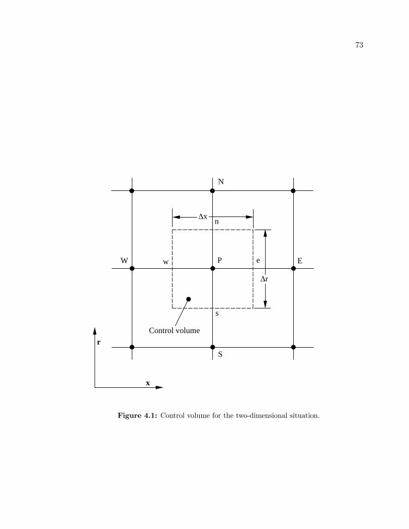
73

P W E

N

S

n

w e

s

∆x

∆r

Control volume

x

r

Figure 4.1: Control volume for the two-dimensional situation.

74

If Sφ is independent of time then Eq. (4.4) becomes

·ρPφP − ρoPφ

oP

∆t− Sφ

¸∆∀+ Je − Jw + Jn − Js = 0 (4.5)

Where Je, Jw, Jn, and Js are the integrated total fluxes over the control volume faces;

i.e., Je stands for Jx∆Ax over the interface e, and so on. Where the superscript ‘o’ is

used for old values (i.e., the values at previous time step).

The linearization of the source term gives

Sφ = So + SPφP (4.6)

Now Eq. (4.5) becomes

µρPφP − ρoPφ

oP

∆t

¶∆∀+ Je − Jw + Jn − Js = (So + SPφP )∆∀ (4.7)

Now integration of the continuity equation (3.1) in a similar manner to Eq. (3.46)

gives

Z t+∆t

t

½ZCV

·∂ρ

∂t+

∂

∂xj(ρeuj)¸ d∀¾ dt = 0 (4.8)

or

Z t+∆t

t

½∂ρ

∂t∆∀+ [ρeuj∆Aj]L2L1¾ dt = 0 (4.9)

75

or

Z t+∆t

t

½∂ρ

∂t∆∀+ [Fj∆Aj ]L2L1

¾dt = 0 (4.10)

or

µρP − ρoP

∆t

¶∆∀+ Fe − Fw + Fn − Fs = 0 (4.11)

Where Fj is the mass flux through the face ‘j’; Fe, Fw, Fn, and Fs are the mass

flow rates through the faces of the control volume; i.e., Fe stands for Fx∆Ax over the

interface e, and so on.

Multiplying Eq. (4.11) by φP , subtracting the resulting equation from Eq. (4.7)

and knowing that;

Je − FeφP = aE(φP − φE) (4.12)

Jw − FwφP = aW (φW − φP ) (4.13)

Jn − FnφP = aN(φP − φN) (4.14)

Js − FsφP = aS(φS − φP ) (4.15)

one can develop the following algebraic equation [81]:

aPφP = aEφE + aWφW + aNφN + aSφS + b (4.16)

76

Where

aP = aE + aW + aN + aS + aoP − SP∆∀ (4.17)

aoP =ρoP∆∀∆t

(4.18)

b = aoPφoP + So∆∀ (4.19)

aE = DeA(|Pe|) + [[−Fe, 0]] (4.20)

aW = DwA(|Pw|) + [[Fw, 0]] (4.21)

aN = DnA(|Pn|) + [[−Fn, 0]] (4.22)

aS = DsA(|Ps|) + [[Fs, 0]] (4.23)

and Pe, Pw, Pn, and Ps are the Peclet numbers: i.e., Pe stands forFeDeand so on; De,

Dw, Dn, and Ds are the diffusion conductances; i.e., De stands forΓe∆y(δx)e

and so on.

The values of A(|P |) are given in [81] for different schemes. In the present study, first

order upwind scheme is employed for which A(|P |) is unity.

Equation (4.16) is written for each of the variables, eu, ev, k, ², eρ, eYi and eT at everycell. Although the control volumes adjacent to the boundary are treated differently

from the interior ones and need different algebraic formulation, it is possible to have a

unified formulation to calculate the field variable in the near boundary region through

the use of source term [75].

77

4.4 Computation of the Flow Field

The solution of the general transport equation (3.46) presents two new problems:

• The convective term of Eq. (3.46) contains non-linear inertia terms.

• The continuity, momentum, energy, species and turbulence equations, repre-

sented by Eq. (3.46), are intricately coupled because every velocity component ap-

pearing in each equation. The most complex issue to resolve is the role played by

pressure. It appears in the momentum equations, but there is evidently no transport

equation for pressure.

If the pressure gradient is known, the process of obtaining and solving discretized

equations for velocities from momentum equations is similar to that for any other

scalar (e.g. temperature, species mass fraction, etc.) and developed schemes such as

central differencing, upwind, hybrid schemes, etc. are applicable. In general purpose

flow computations the pressure field is calculated as a part of the solution so its

gradient is normally not known beforehand. If the flow is compressible the continuity

equation may be used as a transport equation for density, and the pressure may be

obtained from the density and temperature by using the equation of state. However,

if the flow is incompressible the density is constant and hence by definition not linked

to the pressure. In this case coupling between pressure and velocity introduces a

constraint on the solution of the flow field: if the correct pressure field is applied in

the momentum equations the resulting velocity field should satisfy continuity.

Both the problems associated with the non-linearities in Eq. (3.46) and the

78

pressure velocity linkage can be resolved by adopting an iterative solution strategy

such as SIMPLE ( Semi-Implicit Method for Pressure-Linkage Equations) algorithm

of Patankar and Spalding [75].

Before outlining the algorithm it is very important to explain the grid staggering,

which is the first step to the SIMPLE algorithm. The finite volume method starts,

as always, with the discretization of the flow domain and of the general transport

equation (3.46). First there is a need to decide where to store the velocities. It

seems logical to define these at the same locations where the scalar variables, such

as pressure, temperature etc., are defined. However, if the velocities and pressure are

both defined at the nodes of an ordinary control volume, a highly non-uniform pressure

field can act like a uniform field in the discretized momentum equations [75]. For

instance, if velocities and pressure are both defined at the nodes of an ordinary control

volume and the pressure gradient terms in the momentum equations are discretized

by central differencing scheme in a uniformly discretized flow field, it is found that

all the discretized pressure terms in axial and radial directions are zero at all nodal

points even though the pressure field exhibits spatial oscillation in both directions of

a two dimensional flow field [75]. As a result, this pressure field would give the same

(zero) momentum source in the discretized equations as a uniform pressure field. This

behavior is obviously non-physical.

It is clear that, if the velocities are defined at the scalar nodes (at which scalars,

such as pressure and temperature, are defined), the influence of pressure is not prop-

erly represented in the discretized momentum equations. A remedy for this problem

79

is to use a staggered grid for the velocity components. The idea is to evaluate scalar

variables, such as pressure, density, temperature, species concentration, turbulence

kinetic energy and turbulence dissipation, at ordinary nodal points but to calculate

velocity components on staggered grids centered around the cell faces. The arrange-

ment for two-dimensional flow calculation with staggered grid arrangement is shown

in Figure 4.2. In Figure 4.2 unbroken lines (grid lines) are numbered by means of

capital letters ..., I − 1, I, I + 1, ... and ..., J − 1, J, J + 1, ... in the axial and radial

directions respectively whereas the dashed lines that construct the scalar cell faces

are denoted by lower case letters ..., i−1, i, i+1, ... and ..., j−1, j, j+1, ... in the axial

and radial directions respectively. A subscript system based on this numbering allows

us to define the locations of grid nodes and cell faces with precision. Scalar nodes,

located at the intersection of two grid lines, are identified by two capital letters: e.g.

point P in Figure 4.2 is denoted by (I, J). The axial velocities are stored at the e-

and w-cell faces of a scalar control volume. These are located at the interaction of a

line defining a cell boundary and a grid line and are, therefore, defined by a combina-

tion of a lower case letter and a capital: e.g. the w-face of the cell around point P is

identified by (i, J). For the same reasons the storage locations for the radial velocities

are combinations of a capital and a lower case letter: e.g. the s-face is given by (I, j).

The staggering of the velocity avoids the unrealistic behavior of the discretized

momentum equation for spatially oscillating pressures. A further advantage of the

staggered grid arrangement is that it generates velocities at exactly the locations

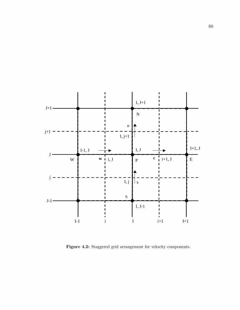
80

i i+1

E W

N

S

I, J+1

I, j

n

I, J-1

s

e w

I, j+1

i+1, J i, J

I+1, J I-1, J

I-1 I I+1

J-1

J

j

j+1

J+1

P

I, J

Figure 4.2: Staggered grid arrangement for velocity components.

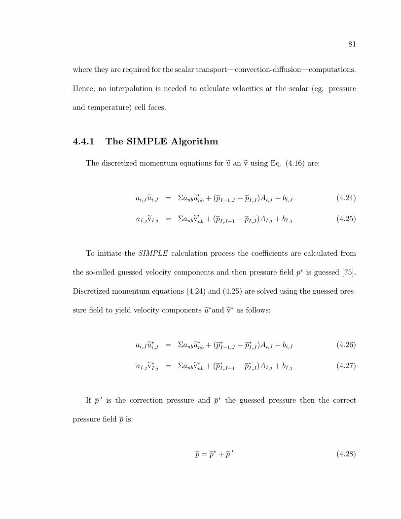
81

where they are required for the scalar transport–convection-diffusion–computations.

Hence, no interpolation is needed to calculate velocities at the scalar (eg. pressure

and temperature) cell faces.

4.4.1 The SIMPLE Algorithm

The discretized momentum equations for eu an ev using Eq. (4.16) are:ai,Jeui,J = Σanbeu0nb + (pI−1,J − pI,J)Ai,J + bi,J (4.24)

aI,jevI,j = Σanbev0nb + (pI,J−1 − pI,J)AI,j + bI,j (4.25)

To initiate the SIMPLE calculation process the coefficients are calculated from

the so-called guessed velocity components and then pressure field p∗ is guessed [75].

Discretized momentum equations (4.24) and (4.25) are solved using the guessed pres-

sure field to yield velocity components eu∗and ev∗ as follows:ai,Jeu∗i,J = Σanbeu∗nb + (p∗I−1,J − p∗I,J)Ai,J + bi,J (4.26)

aI,jev∗I,j = Σanbev∗nb + (p∗I,J−1 − p∗I,J)AI,j + bI,j (4.27)

If p 0 is the correction pressure and p∗ the guessed pressure then the correct

pressure field p is:

p = p∗ + p 0 (4.28)

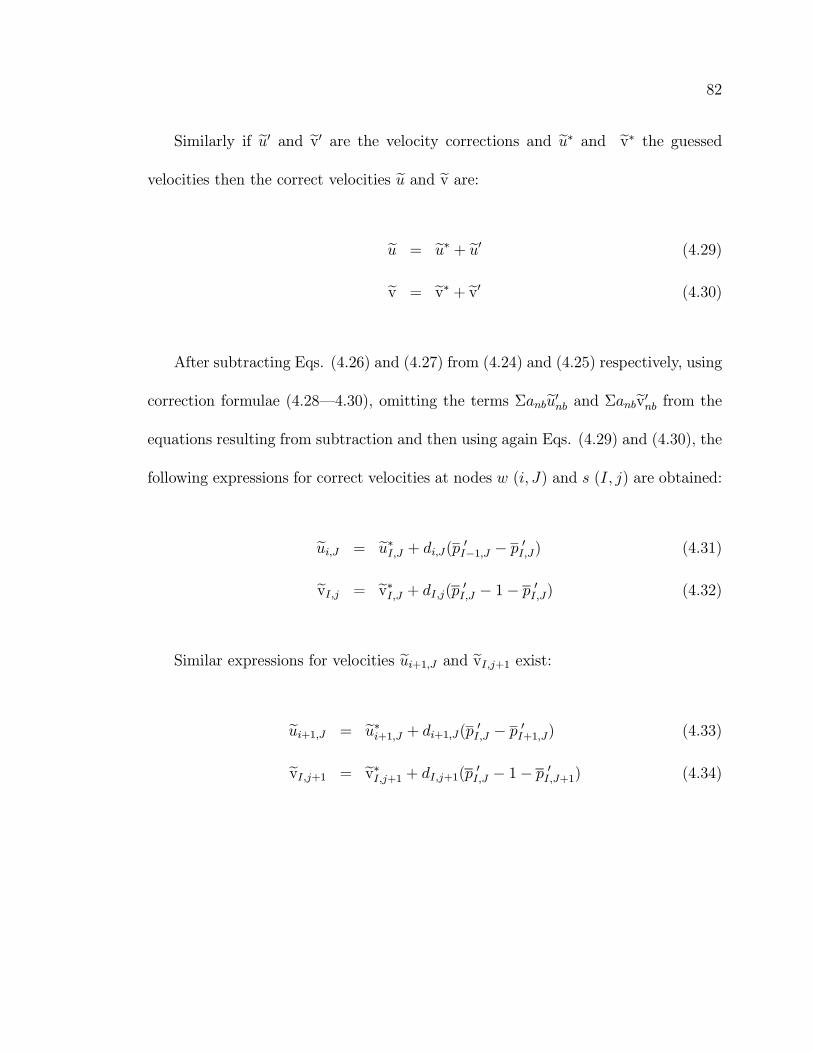
82

Similarly if eu0 and ev0 are the velocity corrections and eu∗ and ev∗ the guessedvelocities then the correct velocities eu and ev are:

eu = eu∗ + eu0 (4.29)

ev = ev∗ + ev0 (4.30)

After subtracting Eqs. (4.26) and (4.27) from (4.24) and (4.25) respectively, using

correction formulae (4.28–4.30), omitting the terms Σanbeu0nb and Σanbev0nb from the

equations resulting from subtraction and then using again Eqs. (4.29) and (4.30), the

following expressions for correct velocities at nodes w (i, J) and s (I, j) are obtained:

eui,J = eu∗I,J + di,J(p 0I−1,J − p 0I,J) (4.31)

evI,j = ev∗I,J + dI,j(p 0I,J − 1− p 0I,J) (4.32)

Similar expressions for velocities eui+1,J and evI,j+1 exist:eui+1,J = eu∗i+1,J + di+1,J(p 0I,J − p 0I+1,J) (4.33)

evI,j+1 = ev∗I,j+1 + dI,j+1(p 0I,J − 1− p 0I,J+1) (4.34)

83

Where

di,J = Ai,J/ai,J (4.35)

dI,j = AI,j/aI,j (4.36)

di+1,J = Ai+1,J/ai+1,J (4.37)

dI,j+1 = AI,j+1/aI,j+1 (4.38)

Using correct velocity in the discretized continuity equation, the following dis-

cretized equation for the pressure correction p 0 is obtained:

aI,Jp0I,J = aI+1,Jp

0I+1,J + aI−1,Jp

0I−1,J + aI,J+1p

0I,J+1 + aI,J−1p

0I,J−1 + b

0I,J (4.39)

Where

aI,J = aI+1,J + aI−1,J + aI,J+1 + aI,J−1 (4.40)

aI+1,J = (ρdA)i+1,J (4.41)

aI−1,J = (ρdA)i,J (4.42)

aI,J+1 = (ρdA)I,j+1 (4.43)

aI,J−1 = (ρdA)I,j (4.44)

b0I,J = (ρeu∗A)i,J − (ρeu∗A)i+1,J + (ρev∗A)I,j − (ρev∗A)I,j+1 (4.45)

As soon as the starred velocity components are obtained the pressure correction

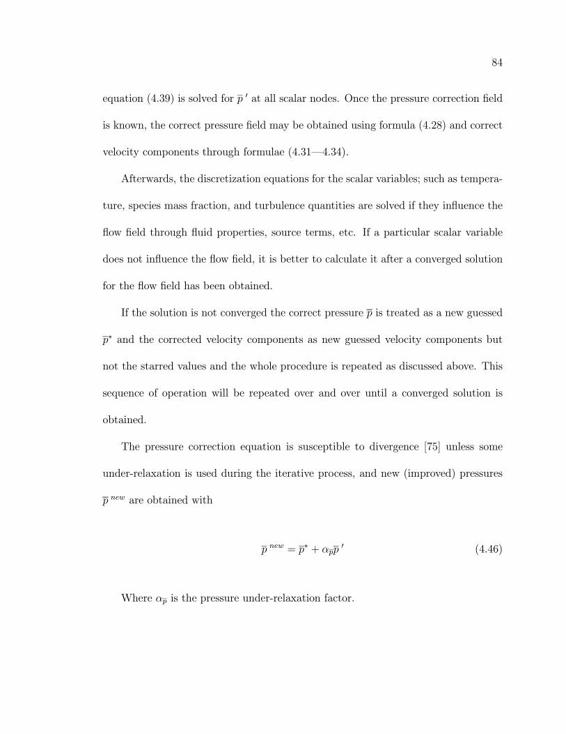
84

equation (4.39) is solved for p 0 at all scalar nodes. Once the pressure correction field

is known, the correct pressure field may be obtained using formula (4.28) and correct

velocity components through formulae (4.31–4.34).

Afterwards, the discretization equations for the scalar variables; such as tempera-

ture, species mass fraction, and turbulence quantities are solved if they influence the

flow field through fluid properties, source terms, etc. If a particular scalar variable

does not influence the flow field, it is better to calculate it after a converged solution

for the flow field has been obtained.

If the solution is not converged the correct pressure p is treated as a new guessed

p∗ and the corrected velocity components as new guessed velocity components but

not the starred values and the whole procedure is repeated as discussed above. This

sequence of operation will be repeated over and over until a converged solution is

obtained.

The pressure correction equation is susceptible to divergence [75] unless some

under-relaxation is used during the iterative process, and new (improved) pressures

p new are obtained with

p new = p∗ + αpp0 (4.46)

Where αp is the pressure under-relaxation factor.

85

The velocities eu∗ and ev∗, and eu and ev are also under-relaxed as follows:eu∗ new = αeueu∗ + (1− αeu)eun−1 (4.47)

ev∗ new = αevev ∗+(1− αev)evn−1 (4.48)

eunew = αeueu+ (1− αeu)eun−1 (4.49)

evnew = αevev + (1− αev)evn−1 (4.50)

αeu and αev are under relaxation factors for x and y velocity components. eu∗ and ev∗are the velocity components obtained from solving the momentum equations (4.26)

and (4.27) whereas eu and ev are the corrected velocity components obtained fromvelocity correction formulae (4.31–4.34). eun−1 and evn−1 are the velocity componentsobtained in the previous iteration.

The pressure correction equation is also affected by velocity under-relaxation and

it can be shown that the d-terms of pressure correction equation (4.39) will be mul-

tiplied by the velocity under-relaxation. The second terms of the velocity correction

formulae (4.31–4.34) will also be multiplied by the velocity under-relaxation.

The whole steps followed can be well described by the flow chart (Fig. 4.3).

86

No

Initialize

Set time step

Set up time independent boundary conditions

Give initial guess to

Set up time dependent boundary conditions

Calculate the coefficients of all the discretized equations

Solve the discretized momentum Eqs. (4.26 ) & (4.27)

Solve the pressure correction Eq. (4.39)

Correct pressure by Eq. (4.28) and velocities by Eqs. (4.31 -- 4.34)

Solve the discretized Eq. (4.16) for the scalar quantities

Convergence?

Yes

Yes

No

t∆

εand,~

,~

,,~,~ kYTpvu i

εand,~

,~

,,~,~ kYTpvu i

εε =======

∆+=oo

io

ioooo kkYYTTppvvuu

ttt

and,~~

,~~

,,~~,~~Let

εand,~

,~

,,~,~ kYTpvu i

** ~,~ vu

/p

**** and,~

,~

,,~,~ εkYTpvu i

εand,~

,~

,,~,~ kYTpvu i

εand,~

,~

kYT i

Stop

Start

maxtt <

vv

uupp~~and

~~,

Set

*

**

===

Figure 4.3: The SIMPLE algorithm.

87

4.5 Grid Details and Computation

4.5.1 Free Transient Turbulent jet

Along the radial direction fine uniform grid spacing is allocated at the inlet (inlet

to control volume) while gradually increased spacing is considered away from it. Along

the axial direction grid spacing is fine near the inlet and the wall but it is gradually

increasing. The grid generated in this case is shown in Figure 4.4. The number

of grid planes used in the radial direction is 40 while 50 grid planes are used in the

axial direction, thus making a total of 2000 grid points. The grid independence test

results for pressure and velocity in case of single species are shown in Figures 4.5

& 4.6 respectively whereas these results for pressure in case of multiple species are

shown in Figures 4.7. It may be observed that for 55 × 45 grid points the results

are almost in agreement with the results of 50 × 40 grid points, i.e., the maximum

pressure and velocity magnitude differences are less than 0.1%.

Six variables in case of single species and nine variables in case of multiple species

are computed at all grid points; these are: either the two velocity components, lo-

cal pressure, two turbulence quantities and temperature or two velocity components,

three species mass fractions, local pressure, temperature and two turbulence quanti-

ties.

88

0.000

0.004

0.008

0.012

0.016

0.020

0.000 0.005 0.010 0.015 0.020 0.025 0.030

Axial Distance (m)

Rad

ial D

ista

nce

(m)

0.0000

0.0008

0.0016

0.0024

0.0000 0.0010 0.0020 0.0030 0.0040

A close-up view of the grids near inlet.

Figure 4.4: Computational domain for grid independent solution of an axisym-metric transient turbulent air/helium jet expanding into initially stag-nant air (grid size: 50x40).

89

101160

101200

101240

101280

101320

101360

0.000 0.005 0.010 0.015 0.020 0.025 0.030

Axial Distance (m)

Pre

ssur

e (P

a)

40x30 Grids

45x37 Grids50x40 Grids

55x45 Grids

Figure 4.5: Grid independent test for pressure along the symmetry axis at r =0 m and t =192.30 microseconds for air jet expanding into initiallystagnant air.

90

0

20

40

60

80

100

0.000 0.005 0.010 0.015 0.020 0.025 0.030

Axial Distance (m)

Vel

ocity

Mag

nitu

de (m

/s)

40x30 Grids45x37 Grids

50x45 Grids55x45 Grids

Figure 4.6: Grid independent test for velocity magnitude along the symmetry axisat r = 0 m and t = 192.30 microseconds for air jet expanding intoinitially stagnant air.

91

101160

101200

101240

101280

101320

101360

0.000 0.005 0.010 0.015 0.020 0.025 0.030

Axial Distance (m)

Pre

ssur

e (P

a)

40x30 Grids

45x37 Grids50x40 Grids

55x45 Grids

Figure 4.7: Grid independent test for pressure along the symmetry axis at r = 0m and t = 192.30 microseconds for helium jet expanding into initiallystagnant air.

92

4.5.2 Unsteady Opposing Jets

Along the radial direction fine uniform grid spacing is allocated at the inlets (inlets

to control volume) while gradually increasing spacing is considered away from them so

that still there is a fine grid distribution near the wall (Wall 2 ) next to the steady air

jet inlet. Along the axial direction grid spacing is fine near inlets and the wall (Wall

1 ) next to the transiently developing jet inlet but it is gradually increasing. The grid

generated in this case is shown in Figure 4.8. The number of grid planes used in the

radial direction is 76 while 57 grid planes are used in the axial direction, thus making

a total of 3996 grid points. The grid independence test results for pressure and axial

velocity are shown in Figures 4.9 and 4.10 respectively. It may be observed that for

62 × 84 grid points the results are almost in agreement with the results of 57 × 76

grid points, i.e., the maximum pressure and axial velocity magnitude differences are

less than 0.1%.

Nine variables are computed at all grid points; these are: two velocity compo-

nents, three species mass fractions, local pressure, temperature and two turbulence

quantities.

93

Axial Distance (m)

0.0 0 0.0 1 0.0 2 0.03 0 .04

0 .00

0 .01

0 .02

0 .03

0 .04

0 .05

Aclose-upviewof the gridsnear inlets

0.0000 0.0005 0.0010 0.0015 0.0020

0.0000

0.0005

0.0010

0.0015

A close-up view of the grids near inlets.

Rad

ial D

ista

nce

(m)

Figure 4.8: Computational domain for grid independent solution of a transientlydeveloping turbulent helium jet opposing the steady turbulent air jet(grid size: 57x76).

94

100000

102000

104000

106000

108000

0.0000 0.0004 0.0008 0.0012 0.0016 0.0020

Axial Distance (m)

Pre

ssur

e (P

a)

35x57 Grids46x68 Grids

57x76 Grids62x84 Grids

Figure 4.9: Grid independent test for pressure along the symmetry axis at r =0 m and t = 192.30 microseconds for helium jet opposing the steadyturbulent air jet.

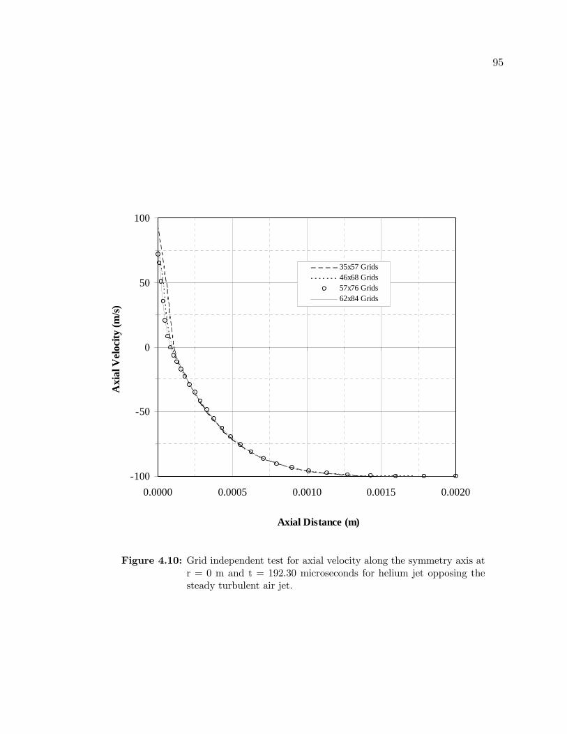
95

-100

-50

0

50

100

0.0000 0.0005 0.0010 0.0015 0.0020

Axial Distance (m)

35x57 Grids46x68 Grids57x76 Grids62x84 Grids

Axi

al V

eloc

ity (m

/s)

Figure 4.10: Grid independent test for axial velocity along the symmetry axis atr = 0 m and t = 192.30 microseconds for helium jet opposing thesteady turbulent air jet.

Chapter 5

RESULTS AND DISCUSSIONS

5.1 Validation of the Model

Since the flow field presented in the present study resembles laser induced vapor

expansion from the cavity, there are no experimental and theoretical studies to vali-

date the present predictions. Therefore, in order to secure the validity of the present

computational model, the simulation conditions are changed in accordance with the

experiment of Kouros et al [41] to justify the capability of the model used in the

present study to predict reasonably. However, the comparison of the prediction with

the result of the above-mentioned experiment will be made after a brief look on the

experimental set-up and the conditions involved in the experiment.

In Figure 5.1 a transparent tank having dimensions 1.2 × 1.2 × 1.5 m deep is

shown, in which the jet flow field is generated by a simple apparatus consisting of a

1.2 m long round clear acrylic tube held in place by a PVC plate at one end. At the

other end, the tube is connected to a fluid feed line and a solenoid valve. The tube,

which has a 28.6 mm inner diameter, is set vertically above the tank such that the

tube exit is just below the water surface. Initially a rubber stopper is placed at the

tube exit (inside the water tank) and dyed fluid is fed into the tube from a reservoir.

96

97

Free water surfaceexposed to atmospheric

pressure

1.2 m

1.5 m

Support plate for thetube

Dimension of thetank into the shownplane is 1.2 m

0.028 m tube with dyed fluid

Tank wallWater Tank

Into the tank

1.2 m

Figure 5.1: Sketch of the experimental set-up [41].

98

Once the tube is filled, the solenoid valve is closed and the fluid is allowed to become

quiescent (1 − 2min.). The rubber stopper is then removed carefully. A minimal

amount of dye (v 5cc) diffused out of the tube prior to the start of the run. The

fluid remains in place by means similar to those which keep a liquid inside a straw

when one end is held airtight. Runs are started when the valve is rapidly opened.

Gravity forces the dyed fluid into the water tank, thus dropping the dyed fluid height

in the tube and as a result generating an unsteady velocity profile at tube exit. The

variations in instantaneous fluid height and unsteady velocity with time obtained by

Kouros et al [41] are shown in Figure 5.2. The maximum tube velocity was found

as 1.86 m/s, resulting in a jet Reynolds number (based on the tube diameter) of

5.3× 104. Hence based on this Reynolds number the jet flow field generated within

the tank is considered turbulent (the instability of the free jets takes place at any

Reynolds number [75]). Since the density difference between the jet dyed fluid and

the tank water is less than 0.1% so the buoyancy effect can be neglected.

Capturing the images of the resulting flow field using the LIF photograph, the

penetration of the tip of the jet was measured at various instants of time and is plotted

against time, which is reproduced in Figure 5.3. In order to compare the variation of

penetration length with time, the standard k − ² model is used. The comparison of

results obtained numerically with the measured values is shown in Figure 5.4. It can

be observed that both results are in good agreement. The error bars are associated

with the experimental errors, which was reported as 3.5%.

99

Figure 5.2: Measured fluid height and calculated velocity of the fluid inside thetube [41].

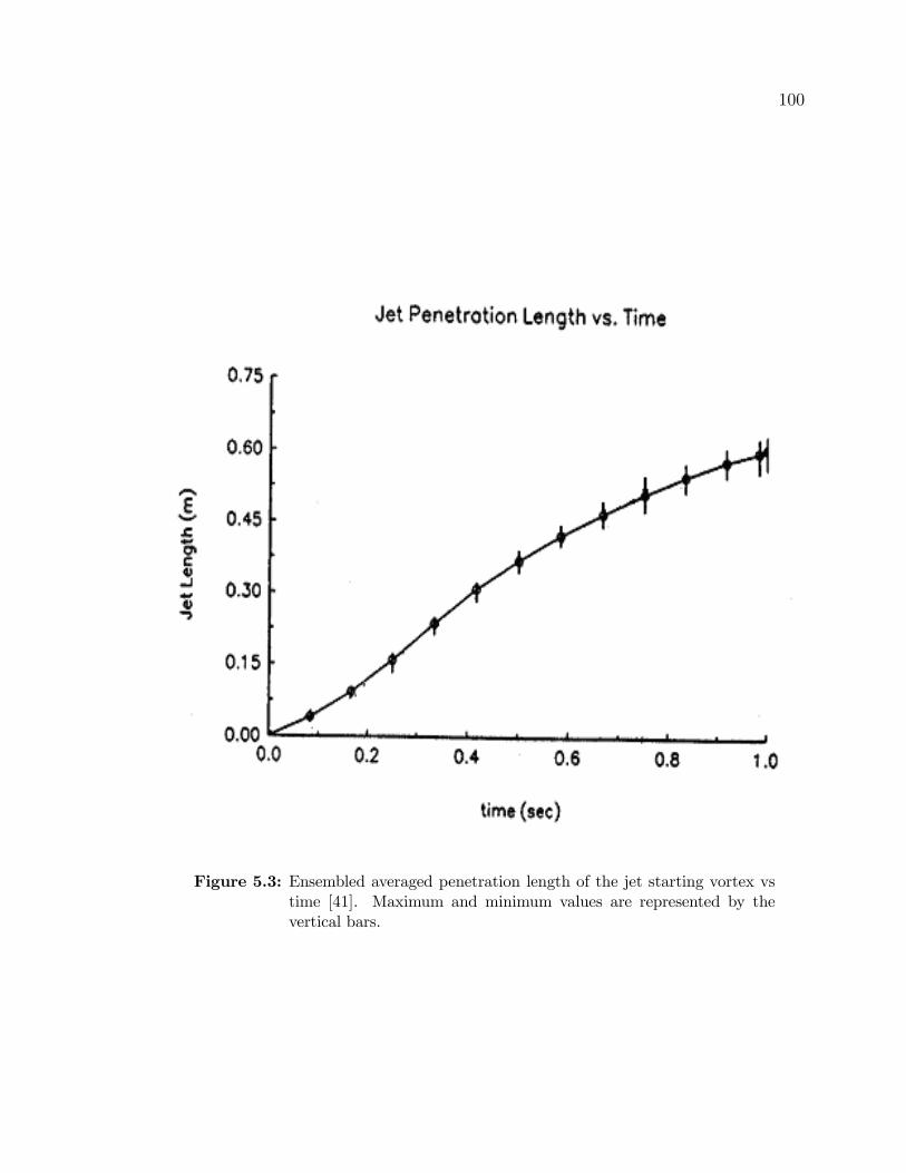
100

Figure 5.3: Ensembled averaged penetration length of the jet starting vortex vstime [41]. Maximum and minimum values are represented by thevertical bars.

101

0.00

0.10

0.20

0.30

0.40

0 0.1 0.2 0.3 0.4 0.5 0.6

Time (s)

Measured [Kouros et al]

Predicted

Jet P

enet

ratio

n L

engt

h (m

)

Figure 5.4: Comparison of numerical predictions with the experimental data forthe case of unsteady turbulent jet entering the water tank [41]. Theerror bars are associated with the experimental error (3.5%) as indi-cated in the previous study [41].

102

5.2 Transient Jet Expansion into Stagnant Air

A transiently developing vapor jet emanating from the solid surface, which is

exposed to laser irradiation, and expanding into an initially stagnant ambient, in

practical applications the ambient is normally air, is simulated to resemble the laser

induced evaporation process. Since the actual vapor properties are not known, the

quantitative results become almost impossible. Therefore, in the first phase of the

present study two gases; air and helium, at 1500 K (imitating the evaporating tem-

perature of the laser-irradiated solid) are employed to resemble the laser-induced

vapor jet expanding into an initially stagnant air ambient. This enforces the assump-

tion that the two gas jets behave like perfect gases. Using the two different gases,

i.e., helium and air, as perfect gases may not give the complete answer; however,

it enables to demonstrate the quantitative behavior of the evaporating front (eject-

ing jet). Moreover, the evaporation of the solid surface causes the vapor jet which

develops spatially and transiently, which implies that the velocity profile of the jet

varies spatially and temporally. In the present study, this velocity profile of the vapor

jet measured previously by Yilbas et al [78] is used as jet exit (inlet to the control

volume) conditions to accommodate in the simulations. Figure 5.5 shows the jet exit

(inlet to the control volume) profiles. Furthermore, since the flow field is actually

generated by high velocity jet expanding into an initially stagnant air, therefore it is

considered turbulent. In order to accommodate turbulence, the standard k− ² model

is used.

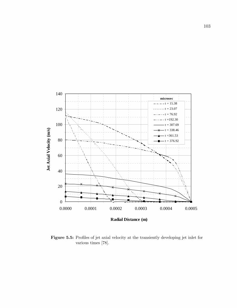
103

microsec

0

20

40

60

80

100

120

140

0.0000 0.0001 0.0002 0.0003 0.0004 0.0005

Radial Distance (m)

Jet A

xial

Vel

ocity

(m/s

)

t = 15.38

t = 23.07

t = 76.92

t =192.30

t = 307.69

t = 338.46

t =361.53

t = 376.92

Figure 5.5: Profiles of jet axial velocity at the transiently developing jet inlet forvarious times [78].

104

5.2.1 Transient Air Jet into Stagnant Air

Figure 5.6 and 5.7 show velocity vectors in the region close to the jet inlet-

expansion region as well as in the radially extended and axially contracted region

at different times. The jet expansion results in the development of the circulation cell

in the region next to the jet outer surface. This is because of the flow entrainment in

this region. The orientation of the circulation cell changes as jet expansion progresses.

This is mainly because of the jet inlet velocity profile, which changes spatially with

time (Fig. 5.5). Therefore, the fluid entrainment varies with time. In the early period

(t ≤ 76.92 µs), jet expands radially more than it does axially; however, as the time

progresses axial expansion dominates over the radial expansion. This is due to: i)

the pressure which builds up close to the jet front region, and ii) the jet inlet velocity

profile which develops radially with time (Fig. 5.5). In this case, as the jet velocity

profiles become almost similar, the axial expansion of the jet is considerable.

Figure 5.8 shows the velocity magnitude contours while Figure 5.9 shows its vari-

ation along the symmetry axis as time variable. In the early period, jet expansion

is not considerable and as the time progresses jet expands radially first and then

expands further along the axial direction. This is because of the jet exit velocity

profile, which develops radially with time, as well as still air resistance opposing the

jet expansion in the axial direction. Flow entrainment is evident after t = 23.07 µs,

in this case, the outer velocity contours differ than those corresponding to earlier

time period. Although the jet penetration extends in the axial direction, velocity

105

Axial Distance (m)

Rad

ialD

ista

nce

(m)

0.0000 0.0010 0.0020 0.0030 0.0040 0.0050

0.0000

0.0005

0.0010

0.0015

t = 15.38 microsec

0.0000 0.0010 0.0020 0.0030 0.0040 0.0050

0.0000

0.0005

0.0010

0.0015

t = 23.07 microsec

0.0000 0.0010 0.0020 0.0030 0.0040 0.0050

0.0000

0.0005

0.0010

0.0015

t = 76.92 microsec

0.0000 0.0010 0.0020 0.0030 0.0040 0.0050

0.0000

0.0005

0.0010

0.0015

t = 192.30 microsec

0.0000 0.0010 0.0020 0.0030 0.0040 0.0050

0.0000

0.0005

0.0010

0.0015

t = 307.69 microsec

0.0000 0.0010 0.0020 0.0030 0.0040 0.0050

0.0000

0.0005

0.0010

0.0015

t = 338.46 microsec

0.0000 0.0010 0.0020 0.0030 0.0040 0.0050

0.0000

0.0005

0.0010

0.0015

t = 361.53 microsec

0.0000 0.0010 0.0020 0.0030 0.0040 0.0050

0.0000

0.0005

0.0010

0.0015

t = 376.92 microsec

Figure 5.6: Time development of velocity vector plots for an axisymmetric tran-sient turbulent air jet close to the jet inlet-expansion region.

106

Axial Distance (m)

Rad

ialD

ista

nce

(m)

0.0000 0.0005 0.0010 0.0015 0.0020

0.0000

0.0005

0.0010

0.0015

0.0020

0.0025

0.0030

t = 376.92 microsec

0.0000 0.0005 0.0010 0.0015 0.0020

0.0000

0.0005

0.0010

0.0015

0.0020

0.0025

0.0030

t = 361.53 microsec

0.0000 0.0005 0.0010 0.0015 0.0020

0.0000

0.0005

0.0010

0.0015

0.0020

0.0025

0.0030

t = 307.69 microsec

0.0000 0.0005 0.0010 0.0015 0.0020

0.0000

0.0005

0.0010

0.0015

0.0020

0.0025

0.0030

t = 338.46 microsec

0.0000 0.0005 0.0010 0.0015 0.0020

0.0000

0.0005

0.0010

0.0015

0.0020

0.0025

0.0030

t = 192.30 microsec

0.0000 0.0005 0.0010 0.0015 0.0020

0.0000

0.0005

0.0010

0.0015

0.0020

0.0025

0.0030

t = 15.38 microsec

0.0000 0.0005 0.0010 0.0015 0.0020

0.0000

0.0005

0.0010

0.0015

0.0020

0.0025

0.0030

t = 23.07 microsec

0.0000 0.0005 0.0010 0.0015 0.0020

0.0000

0.0005

0.0010

0.0015

0.0020

0.0025

0.0030

t = 76.92 microsec

Figure 5.7: Time development of velocity vector plots for an axisymmetric tran-sient turbulent air jet in the radially extended and axially contractedregion.

107

Axial Distance (m)

Rad

ial D

ista

nce

(m)

0.000 0.002 0.004 0.006 0.0080.000

0.001

0.002

0.003(a) t= 15.38 microsec

0.000 0.002 0.004 0.006 0.0080.000

0.001

0.002

0.003(b) t= 23.07 microsec

0.000 0.002 0.004 0.006 0.0080.000

0.001

0.002

0.003(c) t= 76.92 microsec

0.000 0.002 0.004 0.006 0.0080.000

0.001

0.002

0.003(d) t= 192.30 microsec

0.000 0.002 0.004 0.006 0.0080.000

0.001

0.002

0.003(e) t= 307.69 microsec

0.000 0.002 0.004 0.006 0.0080.000

0.001

0.002

0.003( f ) t= 338.46 microsec

0.000 0.002 0.004 0.006 0.0080.000

0.001

0.002

0.003(g) t= 361.53 microsec

0.000 0.002 0.004 0.006 0.0080.000

0.001

0.002

0.003(h) t= 376.92 microsec

Figure 5.8: Time development of velocity magnitude (m/s) contours for an ax-isymmetric transient turbulent air jet expanding into initially stag-nant air.

108

microsec

0

20

40

60

80

100

120

0.000 0.002 0.004 0.006 0.008

Axial Distance (m)

Vel

ocity

Mag

nitu

de (m

/s)

t = 15.38

t = 23.07

t = 76.92

t =192.30

t = 307.69

t = 338.46

t =361.53

t = 376.92

Figure 5.9: Temporal variation of velocity magnitude along the jet symmetry axisat r = 0 m for air jet expanding into initially stagnant air.

109

magnitude reduces considerably with progressing time (Fig. 5.9). This occurs be-

cause of the jet exit velocity profile, where the mean velocity reduces significantly

(Fig. 5.5). The turbulence kinetic energy is high at the jet exit in the early period.

This can be observed from Figure 5.10, in which turbulence kinetic energy along the

symmetry axis is shown. This is because of the jet exit velocity profile. It should be

noted that the turbulence kinetic energy is associated with the jet exit velocity profile

(Eq. (3.34)). The turbulence kinetic energy reduces at jet exit; however, it attains

relatively high values along the symmetry axis during 76.92 ≤ t ≤ 192.30µs. As the

time progresses, its magnitude reduces and does not alter much along the symmetry

axis. This indicates that initial jet expansion results in high degree of turbulence and

once the jet penetration is progressed, the degree of turbulence reduces significantly.

Moreover, changes in jet exit velocity profile results in changes in velocity magnitude

along the symmetry axis. This, in turn, causes large variation in turbulence kinetic

energy, which was also observed in the previous study [82].

Figure 5.11 shows the pressure contours in the region close to the jet expansion

and Figure 5.12 shows the pressure distribution along the symmetry axis. The flow

entrainment and formation of circulation cell is evident from the pressure contours,

which is more visible after t = 76.92 µs. In the early period, jet radial expansion is

more than its axial expansion due to the pressure which builds up close to the jet

inlet region and as time reaches t = 192.30 µs axial expansion of the jet becomes

significant, in which case, the pressure in the jet front region becomes higher than

the jet inlet. This implies the shifting of the pressure peak along the symmetry axis

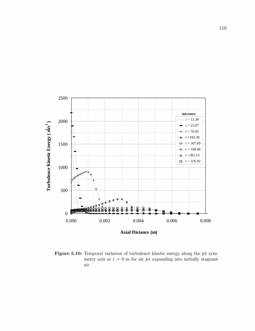
110

microsec

0

500

1000

1500

2000

2500

0.000 0.002 0.004 0.006 0.008

Axial Distance (m)

Tur

bule

nce

Kin

etic

Ene

rgy

( m2 /s

2 ) t = 15.38

t = 23.07

t = 76.92

t =192.30

t = 307.69

t = 338.46

t =361.53

t = 376.92

Figure 5.10: Temporal variation of turbulence kinetic energy along the jet sym-metry axis at r = 0 m for air jet expanding into initially stagnantair.

111

with progressing time (Fig. 5.12). As the jet inlet profile becomes almost similar,

the pressure magnitude along the symmetry axis does not vary considerably, which

in turn results nearly similar pressure profiles along the symmetry axis.

Figure 5.13 shows temperature profiles along the symmetry axis as time variable

while Figure 5.14 shows temperature contours at different times. Temperature profiles

follow almost the profiles of velocity magnitude. This is more pronounced in the early

periods. In this case, convective heat transfer from the jet surface to its ambient is

small due to short period of time and small area of jet surface. As the time progresses,

temperature profiles extend into the jet ambient as follows the jet expansion. When

the jet exit profiles become almost similar in magnitude and shape, the extension of

the temperature profiles into the ambient becomes similar to the case observed for

the unsteady jets [29].

Figure 5.15 shows the dimensionless ratio( ratio of the jet width to penetration

depth) while the logo in the figure shows temporal behavior of penetration depth. The

penetration depth in the early period is low as compared to jet width in the radial

direction. Moreover, as the time progresses, penetration depth becomes larger and the

radial expansion of the jet becomes less than the penetration along the jet symmetry

axis. However, as the time progresses further, jet expansion results in almost self-

similar region as noted in the previous study [29]. In this case D/Zt attains almost

steady decay, which is more pronounced after 250 µs. Moreover, it was shown that

for a fixed jet exit velocity profile a self-similar transient jet could be resulted [29].

Since the gas inlet velocity profiles are varied in the present simulations (in order to

112

Rad

ial D

ista

nce

(m)

Axial Distance (m)

0.000 0.005 0.010 0.015 0.020 0.025 0.0300.000

0.005

0.010

0.015(a) t= 15.38 microsec

0.000 0.005 0.010 0.015 0.020 0.025 0.0300.000

0.005

0.010

0.015(b) t= 23.07 microsec

0.000 0.005 0.010 0.015 0.020 0.025 0.0300.000

0.005

0.010

0.015(c) t= 76.92 microsec

0.000 0.005 0.010 0.015 0.020 0.025 0.0300.000

0.005

0.010

0.015(d) t= 192.30 microsec

0.000 0.005 0.010 0.015 0.020 0.025 0.0300.000

0.005

0.010

0.015(e) t= 307.69 microsec

0.000 0.005 0.010 0.015 0.020 0.025 0.0300.000

0.005

0.010

0.015( f ) t= 338.46 microsec

0.000 0.005 0.010 0.015 0.020 0.025 0.0300.000

0.005

0.010

0.015(g) t= 361.53 microsec

0.000 0.005 0.010 0.015 0.020 0.025 0.0300.000

0.005

0.010

0.015(h) t= 376.92 microsec

Figure 5.11: Time development of pressure (Pa) contours for an axisymmetrictransient turbulent air jet expanding into initially stagnant air.

113

microsec

100800

101200

101600

102000

102400

102800

103200

0.000 0.005 0.010 0.015 0.020 0.025 0.030

Axial Distance (m)

Pre

ssur

e (P

a)

t = 15.38

t = 23.07

t = 76.92

t =192.30

t = 307.69

t = 338.46

t =361.53

t = 376.92

Figure 5.12: Temporal variation of pressure along the jet symmetry axis at r = 0m for air jet expanding into initially stagnant air.

114

microsec

300

500

700

900

1100

1300

1500

0.000 0.002 0.004 0.006 0.008

Axial Distance (m)

Tem

pera

ture

(K)

t = 15.38

t = 23.07

t = 76.92

t =192.30

t = 307.69

t = 338.46

t =361.53

t = 376.92

Figure 5.13: Temporal variation of temperature along the jet symmetry axis at r= 0 m for air jet expanding into initially stagnant air.

115

Rad

ial D

ista

nce

(m)

Axial Distance (m)

0.000 0.002 0.004 0.006 0.008

0.000

0.001

0.002

0.003(a) t= 15.38 microsec

0.000 0.002 0.004 0.006 0.0080.000

0.001

0.002

0.003(b) t= 23.07 microsec

0.000 0.002 0.004 0.006 0.0080.000

0.001

0.002

0.003(c) t= 76.92 microsec

0.000 0.002 0.004 0.006 0.0080.000

0.001

0.002

0.003(d) t= 192.30 microsec

0.000 0.002 0.004 0.006 0.008

0.000

0.001

0.002

0.003(e) t= 307.69 microsec

0.000 0.002 0.004 0.006 0.0080.000

0.001

0.002

0.003( f ) t= 338.46 microsec

0.000 0.002 0.004 0.006 0.0080.000

0.001

0.002

0.003(h) t= 376.92 microsec

0.000 0.002 0.004 0.006 0.0080.000

0.001

0.002

0.003(g) t= 361.53 microsec

Figure 5.14: Time development of temperature (K) contours for an axisymmetrictransient turbulent air jet expanding into initially stagnant air.

116

resemble vapor ejection from the laser-produced cavity), a self- similar region is not

observed clearly in the initial period, except when the jet exit profiles become almost

similar. This corresponds to time period of 350 µs.

Figure 5.16 shows the ratio of penetration depth (Zt) to14power of momentum

rate per unit density³ •MAir /ρ

´. It should be noted that the penetration number is

given as [29]:

Zt³ •MAir /ρ

´1/4×√t

= f(D/Zt) (5.1)

It was reported that for slow flow transient jets, the penetration number remains

constant [29]. It can be observed from Figure 5.16 that the penetration number in-

creases linearly with√t for

√t ≤ 12

õs and beyond this time it changes vastly,

i.e. constant slope of the curve indicates the constant rate of increase in penetration

number. Consequently, in the early period jet behavior is similar to that correspond-

ing to slow flow jet expansion. In this case, the penetration depth is low and the

momentum of the jet is high. As the time progresses, some portion of the jet mo-

mentum is lost due to viscous effect. This in turn reduces the specific momentum

of the jet. Moreover, as the time progresses, the jet penetration rate reduces due to

large diffusion in the region next to the jet front. Although the jet penetration rate

reduces with progressing time, the jet momentum reduces more swiftly because of

the viscous dissipation. Therefore, the rate of momentum loss is considerably higher

than the reduction in penetration rate. This, in turn, results in rapid rise of slope of

117

0.00

0.30

0.60

0.90

1.20

1.50

1.80

0 50 100 150 200 250 300 350 400

Time (ms)

D/Z

t

0.000

0.002

0.004

0.006

0.008

0 50 100 150 200 250 300 350 400

Time (ms)

Zt (

m)

Je t Penetration length of an axisymmetric transient turbulent air jet.

Figure 5.15: Ratio of jet width to penetration length with time for an axisym-metric transient turbulent air jet expanding into initially stagnantair.

118

Figure 5.16: Penetration rate of an axisymmetric transient turbulent air jet exit-ing into initially stagnant air.

119

the curve in the figure for√t ≥ 12√µs.

5.2.2 Transient Helium Jet into Stagnant Air

Figures 5.17 & 5.18 show the velocity vector in the close region of the jet expansion

as well as in the radially extended and axially contracted region at different times.

In the early times, jet expands first radially and then along the axial direction; this

is because of the jet exit velocity profile, which develops radially with time, as well

as stagnant air resistance opposing the jet expansion in the axial direction. Since the

jet inlet velocity profile changes with time, there is no specific pattern of expansion

is observed from the vector plot until after time reaches t = 76.92 µs. As the time

progresses, jet inlet velocity decays so that the jet expansion into its ambient dies.

Moreover, the flow entrainment results in a circulation cell next to the jet boundary,

which is more pronounced after t = 192.30 µs. As the time progresses the orientation

of the circular cell changes and the cell moves away from the jet boundary. As the

time progresses further, the magnitude of jet inlet velocity reduces, the size of the

circulation cell increases. In this case, jet boundary mixes with the secondary flow

generated by the circulation cell.

Figure 5.19 shows the velocity magnitude contours while Figure 5.20 shows its

variation along the symmetry axis as time variable. In the early period, jet expan-

sion is not considerable and as the time progresses jet expands radially first and then

expands further along the axial direction. This is because of the jet exit velocity

profile, which develops radially with time as well as still air resistance opposing the

120

Axial Distance (m)

Rad

ialD

ista

nce

(m)

0.0000 0.0010 0.0020 0.0030

0.0000

0.0005

0.0010

0.0015

t = 15.38 microsec

0.0000 0.0010 0.0020 0.0030

0.0000

0.0005

0.0010

0.0015

t = 23.07 microsec

0.0000 0.0010 0.0020 0.0030

0.0000

0.0005

0.0010

0.0015

t = 76.92 microsec

0.0000 0.0010 0.0020 0.0030

0.0000

0.0005

0.0010

0.0015

t = 192.30 microsec

0.0000 0.0010 0.0020 0.0030

0.0000

0.0005

0.0010

0.0015

t = 307.69 microsec

0.0000 0.0010 0.0020 0.0030

0.0000

0.0005

0.0010

0.0015

t = 338.46 microsec

0.0000 0.0010 0.0020 0.0030

0.0000

0.0005

0.0010

0.0015

t = 361.53 microsec

0.0000 0.0010 0.0020 0.0030

0.0000

0.0005

0.0010

0.0015

t = 376.92 microsec

Figure 5.17: Time development of velocity vector plots for an axisymmetric tran-sient turbulent helium jet close to the jet inlet-expansion region.

121

Axial Distance (m)

Rad

ialD

ista

nce

(m)

0.0000 0.0005 0.0010 0.0015

0.0000

0.0005

0.0010

0.0015

0.0020

t = 15.38 microsec

0.0000 0.0005 0.0010 0.0015

0.0000

0.0005

0.0010

0.0015

0.0020

t = 23.07 microsec

0.0000 0.0005 0.0010 0.0015

0.0000

0.0005

0.0010

0.0015

0.0020

t = 76.92 microsec

0.0000 0.0005 0.0010 0.0015

0.0000

0.0005

0.0010

0.0015

0.0020

t = 192.30 microsec

0.0000 0.0005 0.0010 0.0015

0.0000

0.0005

0.0010

0.0015

0.0020

t = 307.69 microsec

0.0000 0.0005 0.0010 0.0015

0.0000

0.0005

0.0010

0.0015

0.0020

t = 338.46 microsec

0.0000 0.0005 0.0010 0.0015

0.0000

0.0005

0.0010

0.0015

0.0020

t = 361.53 microsec

0.0000 0.0005 0.0010 0.0015

0.0000

0.0005

0.0010

0.0015

0.0020

t = 376.92 microsec

Figure 5.18: Time development of velocity vector plots for an axisymmetric tran-sient turbulent helium jet in the radially expanded and axially con-tracted region.

122

Axial Distance (m)

Rad

ial D

ista

nce

(m)

0.000 0.002 0.004 0.006 0.0080.000

0.001

0.002

0.003(a) t= 15.38 microsec

0.000 0.002 0.004 0.006 0.0080.000

0.001

0.002

0.003(b) t= 23.07 microsec

0.000 0.002 0.004 0.006 0.0080.000

0.001

0.002

0.003(c) t= 76.92 microsec

0.000 0.002 0.004 0.006 0.0080.000

0.001

0.002

0.003(d) t= 192.30 microsec

0.000 0.002 0.004 0.006 0.0080.000

0.001

0.002

0.003(e) t= 307.69 microsec

0.000 0.002 0.004 0.006 0.008

0.000

0.001

0.002

0.003( f ) t= 338.46 microsec

0.000 0.002 0.004 0.006 0.008

0.000

0.001

0.002

0.003(g) t= 361.53 microsec

0.000 0.002 0.004 0.006 0.0080.000

0.001

0.002

0.003(h) t= 376.92 microsec

Figure 5.19: Time development of velocity magnitude (m/s) contours for an ax-isymmetric transient turbulent helium jet expanding into initiallystagnant air.

123

microsec

0

20

40

60

80

100

120

0.0000 0.0008 0.0016 0.0024 0.0032 0.0040

Axial Distance (m)

Vel

ocity

Mag

nitu

de (m

/s)

t = 15.38

t = 23.07

t = 76.92

t =192.30

t = 307.69

t = 338.46

t =361.53

t = 376.92

Figure 5.20: Temporal variation of velocity magnitude along the jet symmetryaxis at r = 0 m for helium jet expanding into initially stagnant air.

124

jet expansion in the axial direction. Flow entrainment is evident after t = 76.92 µs,

in this case, the outer velocity contours differ than those corresponding to earlier

time period. Although the jet penetration extends in the axial direction, velocity

magnitude reduces considerably with progressing time (Fig. 5.20). This occurs be-

cause of the jet exit velocity profile, where the mean velocity reduces significantly

(Fig. 5.5). The turbulence kinetic energy is high at the jet exit in the early period.

This can be observed from Figure 5.21, in which turbulence kinetic energy along the

symmetry axis is shown. This is because of the jet exit velocity profile. It should be

noted that the turbulence kinetic energy is associated with the jet exit velocity profile

(Eq. (3.34)). The turbulence kinetic energy reduces at jet exit; however, it attains

relatively high values along the symmetry axis during 76.92 ≤ t ≤ 192.30µs. As the

time progresses, its magnitude reduces and does not alter much along the symmetry

axis. This indicates that initial jet expansion results in high degree of turbulence and

once the jet penetration is progressed, the degree of turbulence reduces significantly.

Moreover, changes in jet exit velocity profile results in changes in velocity magnitude

along the symmetry axis. This, in turn, causes large variation in turbulence kinetic

energy, which was also observed in the previous study [82].

Figure 5.22 shows the pressure contours in the region close to the jet expansion

and Figure 5.23 shows the pressure distribution along the symmetry axis. The flow

entrainment and formation of circulation cell is evident from the pressure contours,

which is more visible after t = 192.30 µs. In the early period, jet radial expansion

is more than its axial expansion due to the pressure which builds up close to the jet

125

microsec

0

500

1000

1500

2000

2500

0.0000 0.0008 0.0016 0.0024 0.0032 0.0040

Axial Distance (m)

Tur

bule

nce

Kin

etic

Ene

rgy

( m2 /s

2 )

t = 15.38

t = 23.07

t = 76.92

t =192.30

t = 307.69

t = 338.46

t =361.53

t = 376.92

Figure 5.21: Temporal variation of turbulence kinetic energy along the jet sym-metry axis at r = 0 m for helium jet expanding into initially stagnantair.

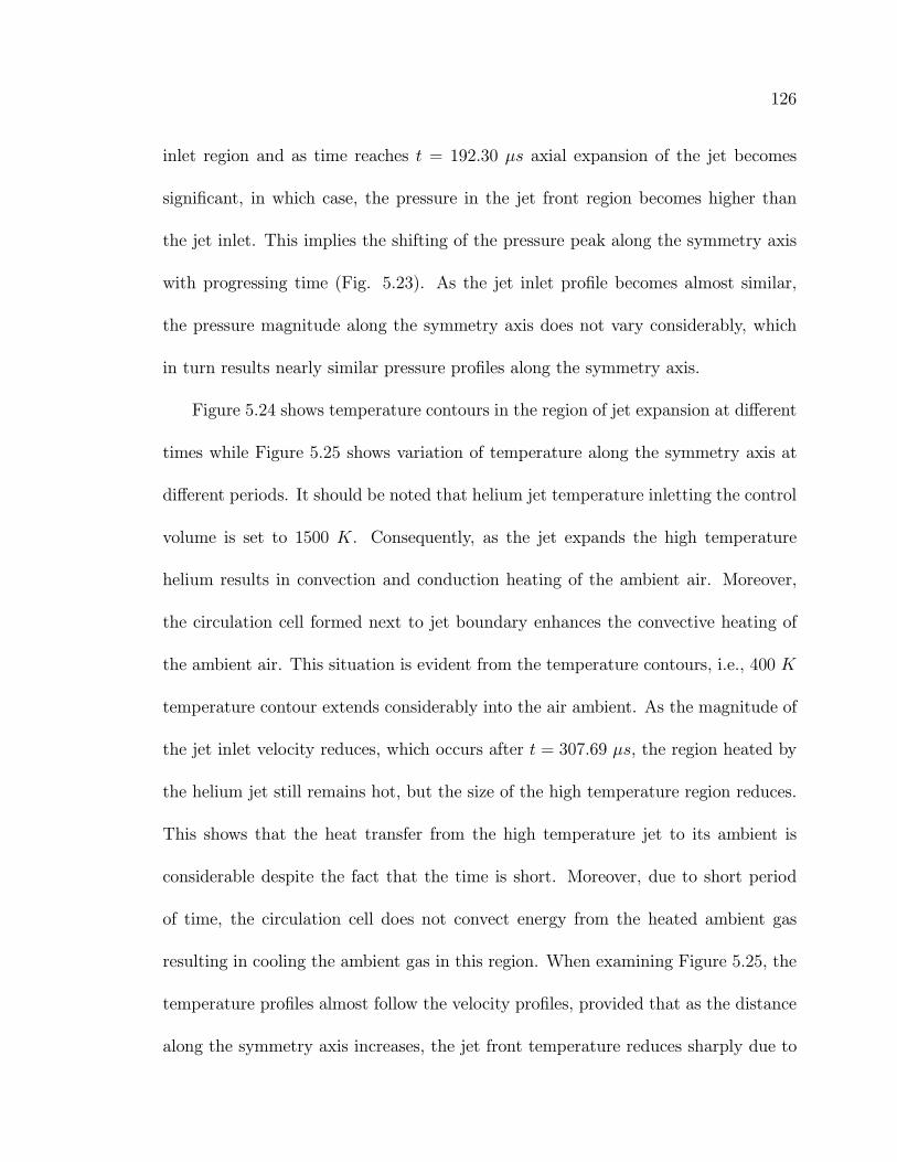
126

inlet region and as time reaches t = 192.30 µs axial expansion of the jet becomes

significant, in which case, the pressure in the jet front region becomes higher than

the jet inlet. This implies the shifting of the pressure peak along the symmetry axis

with progressing time (Fig. 5.23). As the jet inlet profile becomes almost similar,

the pressure magnitude along the symmetry axis does not vary considerably, which

in turn results nearly similar pressure profiles along the symmetry axis.

Figure 5.24 shows temperature contours in the region of jet expansion at different

times while Figure 5.25 shows variation of temperature along the symmetry axis at

different periods. It should be noted that helium jet temperature inletting the control

volume is set to 1500 K. Consequently, as the jet expands the high temperature

helium results in convection and conduction heating of the ambient air. Moreover,

the circulation cell formed next to jet boundary enhances the convective heating of

the ambient air. This situation is evident from the temperature contours, i.e., 400 K

temperature contour extends considerably into the air ambient. As the magnitude of

the jet inlet velocity reduces, which occurs after t = 307.69 µs, the region heated by

the helium jet still remains hot, but the size of the high temperature region reduces.

This shows that the heat transfer from the high temperature jet to its ambient is

considerable despite the fact that the time is short. Moreover, due to short period

of time, the circulation cell does not convect energy from the heated ambient gas

resulting in cooling the ambient gas in this region. When examining Figure 5.25, the

temperature profiles almost follow the velocity profiles, provided that as the distance

along the symmetry axis increases, the jet front temperature reduces sharply due to

127

Axial Distance (m)

Rad

ial D

ista

nce

(m)

0.000 0.005 0.010 0.015 0.020 0.025 0.0300.000

0.005

0.010

0.015(a) t= 15.38 microsec

0.000 0.005 0.010 0.015 0.020 0.025 0.0300.000

0.005

0.010

0.015(b) t= 23.07 microsec

0.000 0.005 0.010 0.015 0.020 0.025 0.0300.000

0.005

0.010

0.015(c) t= 76.92 microsec

0.000 0.005 0.010 0.015 0.020 0.025 0.0300.000

0.005

0.010

0.015(d) t= 192.30 microsec

0.000 0.005 0.010 0.015 0.020 0.025 0.0300.000

0.005

0.010

0.015(e) t= 307.69 microsec

0.000 0.005 0.010 0.015 0.020 0.025 0.0300.000

0.005

0.010

0.015( f ) t= 338.46 microsec

0.000 0.005 0.010 0.015 0.020 0.025 0.0300.000

0.005

0.010

0.015(g) t= 361.53 microsec

0.000 0.005 0.010 0.015 0.020 0.025 0.0300.000

0.005

0.010

0.015(h) t= 376.92 microsec

Figure 5.22: Time development of pressure (Pa) contours for an axisymmetrictransient turbulent helium jet expanding into initially stagnant air.

128

microsec

100800

101200

101600

102000

102400

102800

0.000 0.005 0.010 0.015 0.020 0.025 0.030

Axial Distance (m)

Pre

ssur

e (P

a)

t = 15.38

t = 23.07

t = 76.92

t =192.30

t = 307.69

t = 338.46

t =361.53

t = 376.92

Figure 5.23: Temporal variation of pressure along the jet symmetry axis at r = 0m for helium jet expanding into initially stagnant air.

129

Axial Distance (m)

Rad

ial D

ista

nce

(m)

0.000 0.002 0.004 0.006 0.0080.000

0.001

0.002

0.003(a) t= 15.38 microsec

0.000 0.002 0.004 0.006 0.0080.000

0.001

0.002

0.003(b) t= 23.07 microsec

0.000 0.002 0.004 0.006 0.0080.000

0.001

0.002

0.003(c) t= 76.92 microsec

0.000 0.002 0.004 0.006 0.0080.000

0.001

0.002

0.003(d) t= 192.30 microsec

0.000 0.002 0.004 0.006 0.0080.000

0.001

0.002

0.003(e) t= 307.69 microsec

0.000 0.002 0.004 0.006 0.0080.000

0.001

0.002

0.003( f ) t= 338.46 microsec

0.000 0.002 0.004 0.006 0.0080.000

0.001

0.002

0.003(g) t= 361.53 microsec

0.000 0.002 0.004 0.006 0.0080.000

0.001

0.002

0.003(h) t= 376.92 microsec

Figure 5.24: Time development of temperature (K) contours for an axisymmetrictransient turbulent helium jet expanding into initially stagnant air.

130

microsec

300

500

700

900

1100

1300

1500

0.0000 0.0008 0.0016 0.0024 0.0032 0.0040

Axial Distance (m)

Tem

pera

ture

(K)

t = 15.38

t = 23.07

t = 76.92

t =192.30

t = 307.69

t = 338.46

t =361.53

t = 376.92

Figure 5.25: Temporal variation of temperature along the jet symmetry axis at r= 0 m for helium jet expanding into initially stagnant air.

131

heat transfer from jet to its ambient.

Figures 5.26, 5.27 & 5.28 show mass ratio of helium, nitrogen and oxygen along

the symmetry axis at different times. Depending on the jet expansion, the helium

mass ratio decays sharply along the symmetry axis. However, the deviation in helium

mass ratio at different time is because of the jet inlet velocity profile, which changes

with time (Fig. 5.5). This is particularly true for the early period (t ≤ 76.92 µs).

Figures 5.27 & 5.28 show N2 and O2 mass ratio along the symmetry axis as time

variable. The existence of N2 and O2 indicates the presence of air. The amount of

air present reduces along the symmetry axis as the time period progresses. Moreover,

at the jet inlet air does not mix with helium along the symmetry axis for all times

concerned. However, mixing of air with helium is evident as the distance along the

symmetry axis from the jet inlet increases into the downstream of the jet. This

indicates that while the helium jet expands into the stagnant air, some air molecules

remain in the region close to the jet inlet. In addition, the expansion of helium into

air accelerates the diffusional transport of air into the helium jet.

Figure 5.29 shows mass fraction of helium, nitrogen, and oxygen along the sym-

metry axis at 192.30 µs. Although the mass fraction of helium close to the helium

jet inlet is high, small fraction of nitrogen and oxygen is present there.

The same explanation regarding the enrichment of helium and depletion of nitro-

gen and oxygen along the symmetry axis can be made if mass fraction contours of

helium, nitrogen, and oxygen are considered (Figs. 5.30, 5.31 & 5.32). The only dif-

ference is that the radial expansion of the jet cannot be explained using Figures 5.26,

132

microsec

0.0

0.2

0.4

0.6

0.8

1.0

0.0000 0.0008 0.0016 0.0024 0.0032 0.0040

Axial Distance (m)

Mas

s F

ract

ion

t = 15.38

t = 23.07

t = 76.92

t =192.30

t = 307.69

t = 338.46

t =361.53

t = 376.92

Figure 5.26: Temporal variation of mass fraction of helium along the jet symme-try axis at r = 0 m for helium jet expanding into initially stagnantair.

133

microsec

0.0

0.2

0.4

0.6

0.8

1.0

0.0000 0.0008 0.0016 0.0024 0.0032 0.0040

Axial Distance (m)

Mas

s F

ract

ion

t = 15.38

t = 23.07

t = 76.92

t =192.30

t = 307.69

t = 338.46

t =361.53

t = 376.92

Figure 5.27: Temporal variation of mass fraction of nitrogen along the jet symme-try axis at r = 0 m for helium jet expanding into initially stagnantair.

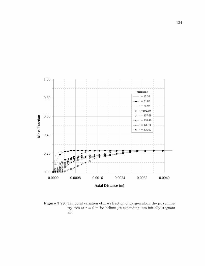
134

microsec

0.00

0.20

0.40

0.60

0.80

1.00

0.0000 0.0008 0.0016 0.0024 0.0032 0.0040

Axial Distance (m)

Mas

s F

ract

ion

t = 15.38

t = 23.07

t = 76.92

t =192.30

t = 307.69

t = 338.46

t =361.53

t = 376.92

Figure 5.28: Temporal variation of mass fraction of oxygen along the jet symme-try axis at r = 0 m for helium jet expanding into initially stagnantair.

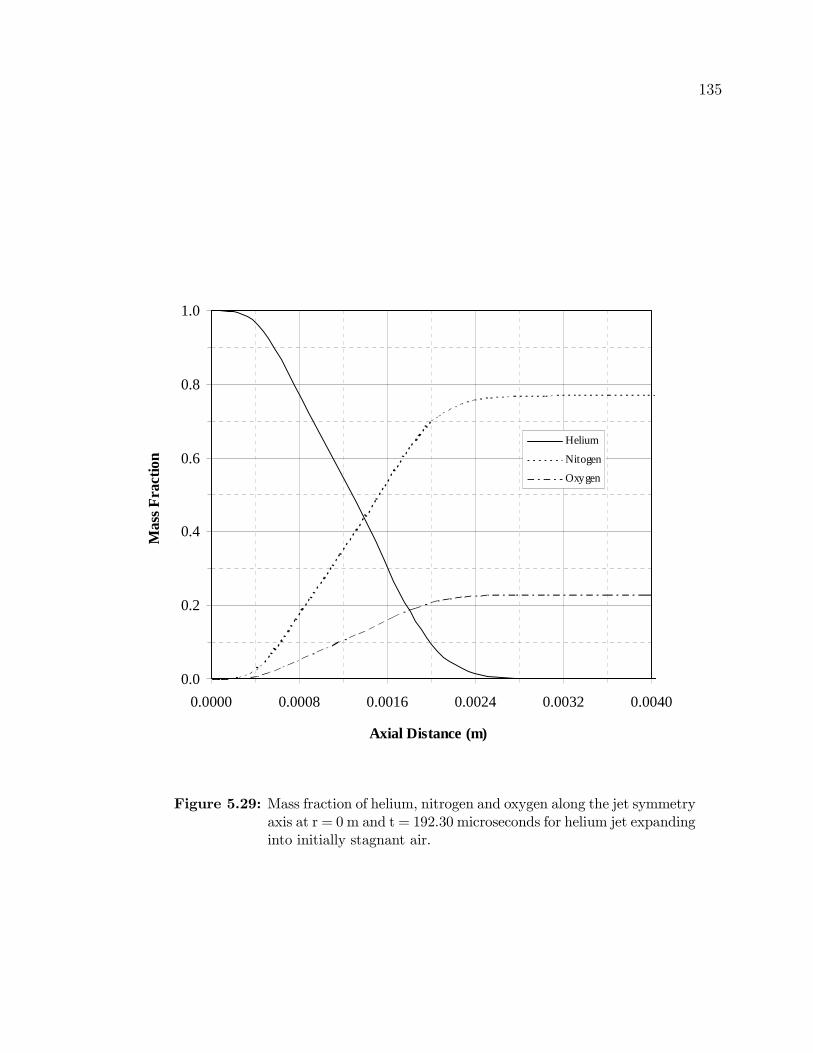
135

0.0

0.2

0.4

0.6

0.8

1.0

0.0000 0.0008 0.0016 0.0024 0.0032 0.0040

Axial Distance (m)

Mas

s F

ract

ion

Helium

Nitogen

Oxygen

Figure 5.29: Mass fraction of helium, nitrogen and oxygen along the jet symmetryaxis at r = 0 m and t = 192.30 microseconds for helium jet expandinginto initially stagnant air.

136

Axial Distance (m)

Rad

ial D

ista

nce

(m)

0.000 0.002 0.004 0.006 0.0080.000

0.001

0.002

0.003(a) t= 15.38 microsec

0.000 0.002 0.004 0.006 0.0080.000

0.001

0.002

0.003(b) t= 23.07 microsec

0.000 0.002 0.004 0.006 0.0080.000

0.001

0.002

0.003(c) t= 76.92 microsec

0.000 0.002 0.004 0.006 0.0080.000

0.001

0.002

0.003(d) t= 192.30 microsec

0.000 0.002 0.004 0.006 0.0080.000

0.001

0.002

0.003(e) t= 307.69 microsec

0.000 0.002 0.004 0.006 0.0080.000

0.001

0.002

0.003( f ) t= 338.46 microsec

0.000 0.002 0.004 0.006 0.0080.000

0.001

0.002

0.003(g) t= 361.53 microsec

0.000 0.002 0.004 0.006 0.0080.000

0.001

0.002

0.003(h) t= 376.92 microsec

Figure 5.30: Time development of mass fraction contours of helium for an ax-isymmetric transient turbulent helium jet expanding into initiallystagnant air.

137

Axial Distance (m)

Rad

ial D

ista

nce

(m)

0.000 0.002 0.004 0.006 0.0080.000

0.001

0.002

0.003(a) t= 15.38 microsec

0.000 0.002 0.004 0.006 0.0080.000

0.001

0.002

0.003(b) t= 23.07 microsec

0.000 0.002 0.004 0.006 0.0080.000

0.001

0.002

0.003(c) t= 76.92 microsec

0.000 0.002 0.004 0.006 0.0080.000

0.001

0.002

0.003(d) t= 192.30 microsec

0.000 0.002 0.004 0.006 0.0080.000

0.001

0.002

0.003(e) t= 307.69 microsec

0.000 0.002 0.004 0.006 0.0080.000

0.001

0.002

0.003( f ) t= 338.46 microsec

0.000 0.002 0.004 0.006 0.0080.000

0.001

0.002

0.003(g) t= 361.53 microsec

0.000 0.002 0.004 0.006 0.0080.000

0.001

0.002

0.003(h) t= 376.92 microsec

Figure 5.31: Time development of mass fraction contours of nitrogen for an ax-isymmetric transient turbulent helium jet expanding into initiallystagnant air.

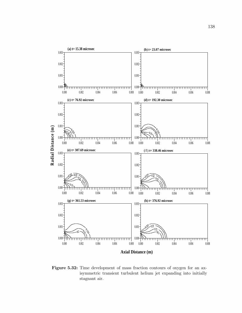
138

Axial Distance (m)

Rad

ial D

ista

nce

(m)

0.000 0.002 0.004 0.006 0.008

0.000

0.001

0.002

0.003(a) t= 15.38 microsec

0.000 0.002 0.004 0.006 0.0080.000

0.001

0.002

0.003(b) t= 23.07 microsec

0.000 0.002 0.004 0.006 0.0080.000

0.001

0.002

0.003(c) t= 76.92 microsec

0.000 0.002 0.004 0.006 0.0080.000

0.001

0.002

0.003(d) t= 192.30 microsec

0.000 0.002 0.004 0.006 0.0080.000

0.001

0.002

0.003(e) t= 307.69 microsec

0.000 0.002 0.004 0.006 0.0080.000

0.001

0.002

0.003( f ) t= 338.46 microsec

0.000 0.002 0.004 0.006 0.008

0.000

0.001

0.002

0.003(g) t= 361.53 microsec

0.000 0.002 0.004 0.006 0.0080.000

0.001

0.002

0.003(h) t= 376.92 microsec

Figure 5.32: Time development of mass fraction contours of oxygen for an ax-isymmetric transient turbulent helium jet expanding into initiallystagnant air.

139

5.27 & 5.28. In the early period, helium jet expansion is not considerable and this

situation is evident by the sharp decay in the mass fraction of helium and sharp rise

in the mass fraction of nitrogen and oxygen close to the jet inlet along the symmetry

axis for t ≤ 23.07 µs. As the time progresses the helium jet expands radially as well as

axially but when time reaches 192.30 µs axial expansion of the jet becomes significant

as compared to the radial expansion. In the later stages of jet expansion, although

the axial expansion rate is faster than the radial expansion rate, large diffusion of

helium jet into the ambient makes the expansion rate in the axial direction slower

than the previous times of dominant axial penetration. This phenomenon enforces

the gradual decay in mass fraction of helium and gradual rise in mass fraction of

nitrogen and oxygen along the symmetry axis.

Figure 5.33 shows the ratio of jet width to penetration length (D/Zt) with time. It

should be noted that D represents the maximum width of the jet while its maximum

axial length is Zt at each time. The transient jet approaches a self-similar configu-

ration with an asymptotic D/Zt ratio. In this case, the jet approaches self-similar

as D/Zt becomes 0.65. The similar situation is observed by Hill and Ouellette [29],

provided that D/Zt obtained is less than the present finding. This is due to different

jet inlet configurations. Moreover, the transition length appears to be about 3 jet

inlet diameters, less than the data reported earlier for steady jet [83]. In the early

period (t ≤ 76.92 µs), jet is transient and it is nowhere self-similar in the flow field.

This is because of the jet inlet velocity profile, which is developing with time as shown

in Figure 5.5. As the jet inlet velocity profiles become almost similar the attainment

140

of self-similarity in the flow field becomes possible.

Figure 5.34 shows the variation of ratio of penetration length (Zt) to14power

of momentum rate per unit density³ •MHe /ρ

´with

√t. The dimensionless quantity

Ztµ •MHe/ρ

¶1/4×√t

represents the penetration number [29,32], where•MHe is the total exit

momentum flow rate. It should be noted that for the transient jet, the penetration is

a linear function of√t, i.e., Ztµ •

MHe/ρ

¶1/4×√t

= constant. It can be observed that during

√t ≤ 14√µs, the slope of the curve remains almost the same. As the time progresses,

the slope of the curve increases and varies with increasing√t. Consequently, to

achieve a constant penetration number during the jet expansion is almost impossible

in the present study, because of variation in momentum flow into the control volume

during the jet expansion. However, the slope of the curve during the period 6√µs ≤

√t ≤ 14√µs is similar to that obtained from the previous study [84].

5.2.3 Comparisons of Results Obtained Due to Transient Air

and Helium Jets

In order to compare the transient jet behavior due to air and helium jets, jet

penetration properties are considered when comparing Figures 5.15 and 5.33 in which

ratio of jet width to penetration length (D/Zt) with time are shown. Although the

behavior of (D/Zt) with time is similar, the slopes of both curves vary considerably.

In this case, the slope of transiently expanding helium jet results in higher slope

[∆(D/Zt)/∆t] than air jet. This indicates that air jet penetrates more into its ambient

141

0.00

0.25

0.50

0.75

1.00

1.25

1.50

1.75

2.00

0 50 100 150 200 250 300 350 400

Time (ms)

D/Z

t

0.0000

0.0010

0.0020

0.0030

0.0040

0 50 100 150 200 250 300 350 400

Time (ms)

Zt (

m)

Je t Penetration length of an axisymmetric transient turbulent helium jet.

Figure 5.33: Ratio of jet width to penetration length with time for an axisymmet-ric transient turbulent helium jet expanding into initially stagnantair.

142

Figure 5.34: Penetration rate of an axisymmetric transient turbulent helium jetexiting into initially stagnant air.

143

than the helium jet. This occurs because of the density of the helium, which is

lower than the air. This can also be observed from temperature curves (Figs. 5.13

& 5.25). In the case of penetration number, both jets behave similarly (Figs.5.34

& 5.16), provided that longer expansion of the air jet results in larger gradientsh∆(Zt/ρ

•M)1/4/∆

√t)i. This, is, again due to the thermophysical properties of the

fluids, which differ considerably. It should be noted that helium has the density

almost 1/10 of air. Consequently, the momentum of helium jet onset of leaving the

solid surface is considerably smaller than that corresponding to air jet, despite the

fact that both jets have the same transiently varying velocity profiles at this location.

Moreover, the specific heat capacity of helium is almost 5 times higher than the air. It

is, therefore, expected that the convective heating of the ambient gas by the transient

jet is higher in the case of helium. Since the inlet momentum of helium jet is lower

than the air jet, this situation is not reflected in temperature contours in the region

next to helium jet (Fig. 5.24).

5.3 Opposing Jets

In practical laser heating process an assisting gas jet coaxial with the laser-heating

source impinges onto the transiently developing vapor jet emanating from the irra-

diated solid surface. In the next phase of the present study, a high temperature

transiently developing helium jet, resembling the vapor ejection from a laser induced

surface, and an opposing steady air jet, resembling the assisting gas jet, are stud-

ied. Since the thermophysical properties of the evaporating surface are not known in

144

the open literature, helium at 1500 K (imitating the evaporating temperature of the

laser-irradiated solid) is considered as the transiently developing jet. This enforces

the assumption that the transiently developing helium and steady air jets behave

like perfect gases. Using helium, which is different from the laser irradiated vapor,

and air at such a high temperature as perfect gases may not give the complete an-

swer; however, it enables to demonstrate the quantitative behavior of the opposing

jets-situation which is caused by the impingement of the assisting gas jet with the

vapor jet. Moreover, the velocity profile of the transiently developing vapor jet mea-

sured previously by Yilbas et al [78] is used as the velocity profile of the transiently

developing helium jet at one inlet to the control volume (inlet 1), and 17th− power

velocity profile is used as the velocity profile of the steady air jet (assisting gas jet)

at the second inlet to the control volume (inlet 2). Figure 5.5 shows the velocity

profiles of the transiently developing vapor jet. Furthermore, since the flow field is

actually generated by the opposing of the high velocity transiently developing helium

and steady air jet and the flow field is mainly of interest in the near wall region,

therefore low Reynolds number k−² model is used to accommodate turbulence in the

simulations. In this phase of the study, the transient effect and the influence of the

assisting gas velocity on the flow, temperature, pressure, and species mass fraction

fields are discussed.

145

5.3.1 Transient Effect on The Flow Field Due to Opposing

Jets

Opposing jet situation resembling the laser gas assisted processing is discussed.

The transiently developing jet resembling the laser-induced vapor plume and the

steady jet impinging onto the transiently developing jet are considered. The geometric

configurations of the jets are selected in accordance with the actual laser processing

conditions.

Figure 5.35 shows velocity vectors in the region close to the transiently developing

jet region for different periods. The transiently developing jet penetrates into steady

opposing jet during the early period (t ≤ 23.07 µs). As the transiently developing

jet size increases in the radial direction, the opposing jet suppresses the penetration

of the jet in the axial direction. In this case, a circulation cell next to the steady

jet boundary and close to the transient jet is developed (t = 76.92 µs). As the time

progresses further (t = 192.30 µs), radial extension of the transiently developing jet

enhances, which in turn accelerates the radial flow in the region close to the solid wall.

Consequently, the orientation of the circulation cell changes and it moves away from

the steady jet boundary. In this case, transiently developing jet velocity develops

further in the radial direction and its velocity profile enables the impinging jet to

spread radially in the region close to the impinging jet. As the time progresses further

(t ≥ 361.53 µs), the average velocity of the transiently developing jet reduces and

the impinging jet suppresses further penetration of the transiently developing jet and

146

enhanced radial flow close to the wall ensures the steady jet expansion in this region.

The radial expansion of the steady jet at t ≥ 361.53 µs is also observed from Figure

5.36, in which velocity magnitude contours are shown. The size of the circulation

cell grows as time progresses. It should be noted that the transiently developing jet

profiles at control volume inlet changes with time. Consequently, its effect on the size

and orientation of the circulation cell varies with time.

Figure 5.37 shows the pressure contours in the region close to the transiently de-

veloping jet. The high magnitude pressure contours extend into the steady jet region

along the axial direction during the early period. This indicates that a triangle like

transiently developing jet velocity profile penetrates deeper into the steady impinging

jet. As the time progresses, the transiently developing jet expands radially, which

in turn influences streamline curvature of the steady impinging jet. Consequently,

transiently developing jet penetration into the steady jet region is suppressed by

the stagnation region developed in the vicinity of transiently developing jet bound-

ary. This enhances the development of the radial flow; therefore, a circulation cell

is formed next to the steady jet boundary, provided that the pressure field gradu-

ally reduces in this region. In the case of t = 376.92 µs, the appearance of pressure

contour (101.270 KPa) may suggest the formation of the secondary cell close to the

developing jet boundary. However, close examination of velocity contours and ve-

locity vectors indicate that the flow mixing in this region occurs and formation of

secondary cell is unlikely.

Figure 5.38 shows helium mass fraction contours in the region close to the tran-

147

Rad

ialD

ista

nce

(m)

A xial D istance (m)

0.0000

0.0005

0.0010

0.0015

0.0020

0.0025

0.0030

0.0035

15.38 microsec 23.07 microsec 76.92 microsec

0.0000

0.0005

0.0010

0.0015

0.0020

0.0025

0.0030

0.0035

192.30 microsec 307.69 microsec 338.46 microsec

0.0000 0.0005 0.0010 0.0015 0.0020

0.0000

0.0005

0.0010

0.0015

0.0020

0.0025

0.0030

0.0035

361.53 microsec

0.0000 0.0005 0.0010 0.0015 0.0020

369.23 microsec

0.0000 0.0005 0.0010 0.0015 0.0020

376.92 microsec

Figure 5.35: Time development of velocity vector plots of He-air mixture for anaxisymmetric transiently developing helium jet opposing the steadyair jet at air jet velocity of 100 m/s.

148

A xial D istance (m)

Rad

ialD

ista

nce

(m)

6 8

15

3560

6

4

759040.000

0.001

0.002

0.003

0.004

0.005

15.38 microsec

6 8

15

356015 10

90

23.07 microsec

815 10

90

45

60

6

75

2535

45 60

76.92 microsec

88

15

45

60

75 90

6

60

10

35

25

0.000

0.001

0.002

0.003

0.004

0.005

192.30 microsec

6

815

25

45

9075

6

60

3510

45

60

307.69 microsec

6

8

25

9075

4535

6

45

1015

60

338.46 microsec

6

8

6

15

10

25

75 9045

35

45

60

0.000 0.001 0.002

0.000

0.001

0.002

0.003

0.004

0.005

361.53 microsec

6

15

25

60 75

35

45

810

9060

6

0.000 0.001 0.002

369.23 microsec

6

15

25

60 75

35

45

810

9060

0.000 0.001 0.002

376.92 microsec

Figure 5.36: Time development of velocity magnitude (m/s) contours of He-airmixture for an axisymmetric transiently developing helium jet op-posing the steady air jet at air jet velocity of 100 m/s.

149

Rad

ialD

ista

nce

(m)

A xial D istance (m)

102600

101830

102000

102204101190

0.000

0.001

0.002

0.003

0.004

0.005

15.38 microsec

1010

70

1012

68

102600101190

101190

101268

101140

0.000

0.001

0.002

0.003

0.004

0.005

192.30 microsec

101830

102200

102600

101485102000

23.07 microsec

101315101290

101270101315

101190

101485

102600

307.69 microsec

101315

101485101315

101290

101190

102600

101270

101360338.46 microsec

101190

101290

101290

101270

101270

101315

101640102600 101315

0.000 0.001 0.002

369.23 microsec

101190

101290

101290

101270

101270

101315

101640102600 101315

0.000 0.001 0.002

376.92 microsec

101190

10127010

1290

101315

101315

101315

101640

101315

101360

102600

0.000 0.001 0.002

0.000

0.001

0.002

0.003

0.004

0.005

361.53 microsec

101360

101190

101400

101315

101390

102600

76.92 microsec

Figure 5.37: Time development of pressure (Pa) contours of He-air mixture for anaxisymmetric transiently developing helium jet opposing the steadyair jet at air jet velocity of 100 m/s.

150

siently developing jet. In the early time when transiently developing jet axially ex-

tends into the steady impinging jet, helium mass fraction is higher close to the tran-

siently developing jet entering region. As the time progresses, radial expansion of

the transient jet and flow mixing in the region next to the transient jet boundary

lower the helium mass fraction while increase the nitrogen mass fraction (Fig.5.39).

Moreover, mass fraction of helium is suppressed further by the steady impinging jet

for t = 376.92 µs. In the case of nitrogen mass fraction (Fig.5.39), nitrogen mass

fraction reduces in the region close to the transient jet. This is more pronounced in

the early times. Moreover, flow mixing close to the transient jet boundary enhances

the nitrogen mass fraction in this region, which is clearly observed for t ≥ 307.69 µs.

It should be noted that the impinging steady jet is air, which composes of oxygen

and nitrogen. The presence of nitrogen indicates the presence of air in the flow field.

Figure 5.40 shows temperature contours in the region close to the transient jet.

Transiently developing helium jet is at 1500 K at the onset of emanating from the

wall (cavity wall) while steady impinging jet temperature is 300 K at the jet entry.

Consequently, transiently developing jet core temperature remains high while at the

mixing region temperature of the steady jet increases due to the convective and

conductive heat transfer in the mixing region. In the early period t = 15.38 µs,

although the transient jet expands axially into the steady jet, temperature across

the transient jet boundary does not attain high values. Moreover, transient jet core

temperature extends further into the steady jet at t = 23.07 µs. Due to radial

extension of the transiently developing jet and modification of streamline curvature

151

A xial D istance (m)

Rad

ialD

ista

nce

(m)

0.1850.300

0.450

0.065

0.00000

0.00025

0.00050

0.00075

0.00100

15.38 microsec

0.065

0.185

0.950

0.700

0.300

23.07 microsec

0.185

0.3000.4500.700

0.1250.950

76.92 microsec

0.065

0.1250.1 850 .5500.80

0

0 .37

5

0.00000

0.00025

0.00050

0.00075

0.00100

192.30 microsec

0.065

0.125

0.7 0

0 0 .3 7

5 0.185

307.69 microsec

0.7 0

0

0 . 300

0.065

0.125

0.4 5

0

0.1 85

338.46 microsec

0.065

0.185

0 .125

0.70

0

0.375

0.00000 0.00005 0.00010

0.00000

0.00025

0.00050

0.00075

0.00100

361.53 microsec

0.185

0.125

0.70

0

0.3 75

0.065

0.00000 0.00005 0.00010

369.23 microsec

0.185

0.125

0.70

0

0 .375

0.065

0.00000 0.00005 0.00010

376.92 microsec

Figure 5.38: Time development of mass fraction contours of helium in He-air mix-ture for an axisymmetric transiently developing helium jet opposingthe steady air jet at air jet velocity of 100 m/s.

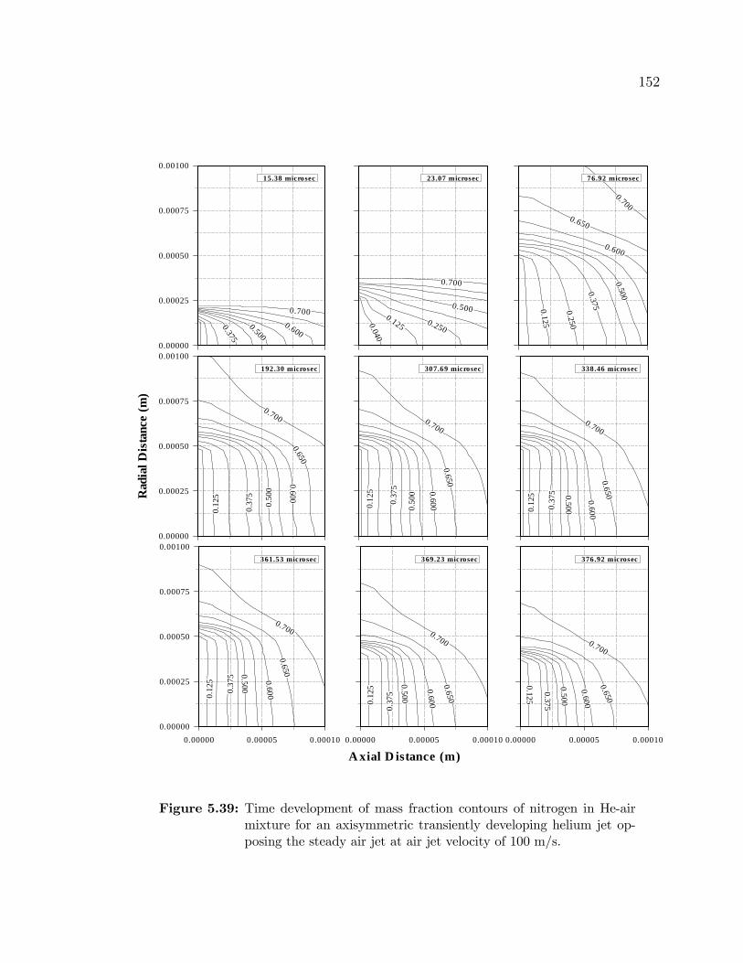
152

Rad

ialD

ista

nce

(m)

A xial D istance (m)

0.600

0.500

0.375

0.700

0.00000

0.00025

0.00050

0.00075

0.00100

15.38 microsec

0.125 0.250

0.500

0.700

0.040

23.07 microsec

0.650

0.600

0.5000.3750.250

0.125

0.700

76.92 microsec

0.700

0.6500.600

0.50

0

0.1 2

5

0.37

5

0.00000

0.00025

0.00050

0.00075

0.00100

192.30 microsec

0.650

0.60 00 .50

0

0 .37

5

0 .1 2

5

0.700

307.69 microsec

0.700

0.600

0 .50 00.37

5

0.12

5

0.6 50

338.46 microsec

0.6500. 5000.3 7

5 0 .60 0

0.700

0.1 2

5

0.00000 0.00005 0.00010

0.00000

0.00025

0.00050

0.00075

0.00100

361.53 microsec

0.700

0.650

0 .60 00.1 2

5

0.37

5

0.5 00

0.00000 0.00005 0.00010

369.23 microsec

0.700

0.650

0.600

0.500

0.125

0 .375

0.00000 0.00005 0.00010

376.92 microsec

Figure 5.39: Time development of mass fraction contours of nitrogen in He-airmixture for an axisymmetric transiently developing helium jet op-posing the steady air jet at air jet velocity of 100 m/s.

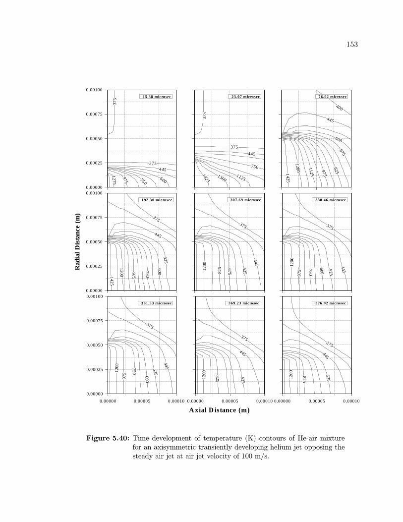
153

A xial D istance (m)

Rad

ialD

ista

nce

(m)

375

375445

600

975

1275 7500.00000

0.00025

0.00050

0.00075

0.00100

15.38 microsec

375

1425

13001125

750

445

375

23.07 microsec

1 42 5

1280 1125

975

825675

600

445

400

76.92 microsec

1 42 5

1200 97 5

7 50

445

375

600525

0.00000

0.00025

0.00050

0.00075

0.00100

192.30 microsec1 2

0 0

825 5 25

445

375

675

307.69 microsec

975

7 5 0

6 00

525

445

375

1200

338.46 microsec

9 75 60 0

445525

375

1200 7 5 0

0.00000 0.00005 0.00010

0.00000

0.00025

0.00050

0.00075

0.00100

361.53 microsec

8 25

525

445

375

1200

0.00000 0.00005 0.00010

369.23 microsec

825

5 25445

375

1200

0.00000 0.00005 0.00010

376.92 microsec

Figure 5.40: Time development of temperature (K) contours of He-air mixturefor an axisymmetric transiently developing helium jet opposing thesteady air jet at air jet velocity of 100 m/s.

154

of the steady jet, temperature field is modified considerably with progressing time.

In this case, flow mixing enhances the temperature rise in the region close to the

transiently developing jet.

Figure 5.41 shows velocity magnitude ratio with x/bj along the symmetry axis for

different periods. It should be noted that ”bj” represents the half velocity width of

the jet and the axial distance is measured from the steady air jet inlet. Moreover, x/bj

remains constant along the symmetry axis for free jets [85]. The steady impinging jet

expands gradually along the symmetry axis, since velocity magnitude ratio remains

almost the same for x/bj ≤ 5. Due to the transiently developing jet, steady jet

expansion in axial direction is suppressed. In this case, radial expansion of steady jet

occurs as observed from Figure 5.36. This results in radial jet emanating from the

region where steady and transiently developing jets meet. Although the transiently

developing jet modifies the flow structure around the jets-meeting-region, the radial

jet behaves like almost a steady jet. Consequently, x/bj ratio remains constant with

velocity magnitude ratio as consistent with the previous work [56].

Figure 5.42 shows the ratio of jet width to penetration length (D/Zt) of the

transiently developing jet. ”D” represents the maximum width of the jet and the

maximum jet height in axial direction is Zt. It should be noted that the transient

jet approaches the self-similar situation when D/Zt remains almost constant with

time. In the present case, transiently developing jet does not approach a self-similar

situation at any time. The sharp increase in D/Zt represents the radial expansion of

the jet due to the opposing steady jet. Once the developing jet reaches a stage where

155

0.4

0.6

0.8

1.0

1.2

0 2 4 6 8

Axial Distance/Half Velocity Width

Vel

ocity

Mag

nitu

de/M

ax. A

ir J

et V

eloc

ity

t = 76.92t = 192.30t = 307.69t = 361.53t = 376.92

microsec

Figure 5.41: Velocity magnitude ratio with dimensionless axial distance measuredfrom the steady air jet inlet at r = 0 m.

156

0

5

10

15

20

25

0 50 100 150 200 250 300 350 400

Time (ms)

D/Z

t

0.00000

0.00008

0.00016

0.00024

0.00032

0.00040

0 50 100 150 200 250 300 350 400

Time (ms)

Zt (m

)

Je t Penetration length of an axisymmetric opposing transiently developing helium jet.

Figure 5.42: Ratio of jet width to penetration length with time for an axisym-metric transiently developing helium jet opposing the steady air jet.

157

the radial expansion of the jet remains almost steady; in which case, penetration of

transiently developing jet in the axial direction is suppressed by the opposing steady

jet. The decaying of D/Zt with time attributes to the decaying of the transiently

developing jet as can also be observed from Figure 5.5, i.e., the mean velocity of the

transiently developing jet decays and its magnitude reduces gradually to zero.

Figure 5.43 shows the variation of ratio of penetration length (Zt) to14power

of momentum rate per unit density³ •MHe /ρ

´with

√t. The dimensionless quantity

Ztµ •MHe/ρ

¶1/4×√t

represents the penetration number [29,32], where•MHe is the total exit

momentum flow rate at the transiently developing jet inlet. It should be noted that the

penetration number remains constant for self-developing transient jets. In the present

situation, the penetration number attains almost steady value during 10 − 15√µs.

This period corresponds to the transiently developing jet entering velocity profiles

being similar (Fig. 5.5). Moreover, sharp increase in the penetration number during

√t ≤ 5

õs represents the axial penetration of the jet, which is significant in the

early periods as can be observed from Figure 5.36. This is also evident from Figure

5.44, in which the ratio of total momentum flow rates corresponding to transiently

developing and steady jets. In this case the momentum ratio increases sharply in

the early period and increases steadily during 7.5 ≤ √t ≤ 12.5√µs. Despite the fact

that the momentum flow rate increases sharply in the early period and it is inversely

proportional to the penetration number, substantial increase in Zt enables to increase

the penetration number during the period√t ≤ 5√µs.

158

Figure 5.43: Penetration rate of an axisymmetric transiently developing heliumjet opposing the steady air jet.

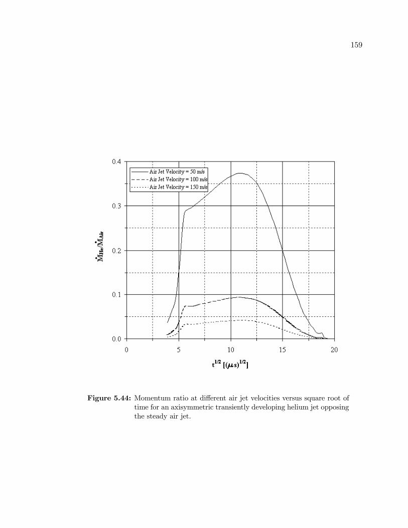
159

Figure 5.44: Momentum ratio at different air jet velocities versus square root oftime for an axisymmetric transiently developing helium jet opposingthe steady air jet.

160

5.3.2 Influence of Assisting Gas Velocity on The Flow Field

Due to Opposing Jets

In order to examine the influence of the magnitude of steady jet mean velocity

on the flow field due to transiently developing opposing jet, the mean velocity of

the steady impinging jet is varied. In order to simplify the arguments, the results

obtained for the flow field at time t = 192.30 µs are presented in the figures. It

should be noted that at t = 192.30 µs, transiently developing jet profiles at the onset

of entering the control volume is almost developed in size (Fig. 5.5).

Figure 5.45 shows velocity vectors for different mean entering velocity of the

steady jet at t = 192.30 µs. In the case of low jet velocity (5 m/s) transiently devel-

oping jet expands axially into the steady jet and the radial expansion of the jet is not

considerable. Therefore, a weak circulation cell radially away from the transiently

developing jet is developed. As the mean velocity of the steady jet increases, axial

expansion of the transiently developing jet is suppressed and due to the streamline

curvature effect of the steady impinging jet, radial flow next to the transiently devel-

oping jet is developed. The strength of the circulation cell increases, which in turn

enhances the flow mixing next to the transiently developing jet boundary. Moreover,

as the mean velocity of the steady jet increases further, the orientation of the cir-

culation cell changes due to the enhancement of the radial flow entrainment. The

strength of the circulation cell increases while the radial expansion of the transiently

developing jet becomes considerable. In this case axial expansion of the transiently

161

Axial Distance (m)

Rad

ialD

ista

nce

(m)

0.0000 0.0005 0.0010 0.0015 0.0020

0.0000

0.0005

0.0010

0.0015

0.0020

0.0025

0.0030

0.0035

Airjet velocity50 m/s

0.0000 0.0005 0.0010 0.0015 0.0020

0.0000

0.0005

0.0010

0.0015

0.0020

0.0025

0.0030

0.0035

Airjet velocity100 m/s

0.0000 0.0005 0.0010 0.0015 0.0020

0.0000

0.0005

0.0010

0.0015

0.0020

0.0025

0.0030

0.0035

Airjet velocity150 m/s

0.0000 0.0005 0.0010 0.0015 0.0020

0.0000

0.0005

0.0010

0.0015

0.0020

0.0025

0.0030

0.0035

Airjet velocity5 m/s

Figure 5.45: Velocity vector plots for four air jet velocities at 192.30 microseconds.

162

developing jet becomes minimum. This can also be seen from Figure 5.46, in which

contours of velocity magnitude are shown. The flow mixing next to the transiently

developing jet boundary is evident for 50 m/s mean velocity of the steady jet.

Figure 5.47 shows helium contours for different mean velocity of the steady jet

at 192.30 µs. In the case of low mean velocity (5 m/s), the axial expansion of

the transiently developing jet enables helium to penetrate into the steady impinging

jet. Consequently, helium mass fraction attains considerably high values along the

symmetry axis. It should be noted that steady impinging jet is air while transiently

developing jet is helium. Moreover, existing of air in the helium jet is not observed.

As the steady impinging jet velocity increases (50 m/s), helium penetration into air

along the axial direction is suppressed and mixing of the air with helium next to the

transiently developing jet boundary reduces the helium mass fraction in this region.

As the steady impinging jet velocity increases further, helium penetration into air

is suppressed considerably. The streamline curvature of the steady impinging jet

enhances the mixing of helium with air in both axial and radial directions.

Figure 5.48 shows temperature contours for different entering mean velocity of

steady jet at t = 192.30 µs. It should be noted that the helium jet is at 1500 K

while the steady impinging jet is at 300 K. Consequently, as transiently developing

jet expands into the steady jet, temperature of air increases in the region close to

the transiently developing jet boundary. This situation is clearly observed for 5 m/s

steady jet velocity. In this case, convection and conduction heating of the air take

place. When the mean velocity of the steady jet increases, flow mixing modifies the

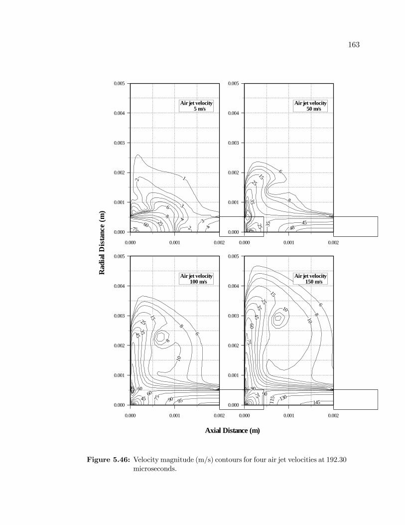
163

Axial Distance (m)

Rad

ialD

ista

nce

(m)

1

3

4

6

8

60

25

4

3

2

275

0.000 0.001 0.002

0.000

0.001

0.002

0.003

0.004

0.005

Airjet velocity5 m/s

6

8

25

2515

35

35 4548

0.000 0.001 0.002

0.000

0.001

0.002

0.003

0.004

0.005

Airjet velocity50 m/s

6

8

8

10

15

25

35

907545

6060

45

95

0.000 0.001 0.002

0.000

0.001

0.002

0.003

0.004

0.005

Airjet velocity100 m/s

68

10

15

2535

4560

75

145115

9090

130

75

10

0.000 0.001 0.002

0.000

0.001

0.002

0.003

0.004

0.005

Airjet velocity150 m/s

Figure 5.46: Velocity magnitude (m/s) contours for four air jet velocities at 192.30microseconds.

164

Axial Distance (m)

Rad

ialD

ista

nce

(m)

0.185

0.125

0.375

0.550

0.650

0.800

0.9000.950

0.065

0.00000 0.00005 0.00010

0.00000

0.00025

0.00050

0.00075

0.00100

Airjet velocity50 m/s

0.065

0.125

0.185

0 .2 50

0.375

0.80

0

0.95

0

0 .55

00.65

0

0.00000 0.00005 0.00010

0.00000

0.00025

0.00050

0.00075

0.00100

Airjet velocity100 m/s

0.1250.185

0 .3 7

5

0.55

0

0.95

0

0.65

0 0.25 0

0.065

0.00000 0.00005 0.00010

0.00000

0.00025

0.00050

0.00075

0.00100

Airjet velocity150 m/s

0.125

0.999

0.800

0.375

0.980

0.065

0.185

0.00000 0.00005 0.00010

0.00000

0.00025

0.00050

0.00075

0.00100

Airjet velocity5 m/s

Figure 5.47: Mass fraction contours of helium for four air jet velocities at 192.30microseconds.

165

Axial Distance (m)

Rad

ialD

ista

nce

(m)

1400

800

600

525

445

375

1200

100 0

0.00000 0.00005 0.00010

0.00000

0.00025

0.00050

0.00075

0.00100

Airjet velocity100 m/s

1 40 0

1200

1000

800

700600

525

445

375

0.00000 0.00005 0.00010

0.00000

0.00025

0.00050

0.00075

0.00100

Airjet velocity150 m/s

445

1497

1495

1485

800

1200

525

1400

0.00000 0.00005 0.00010

0.00000

0.00025

0.00050

0.00075

0.00100

Airjet velocity5 m/s

1425

1350

1200

1050 925850

700

600525

445

375

1400

0.00000 0.00005 0.00010

0.00000

0.00025

0.00050

0.00075

0.00100

Airjet velocity50 m/s

Figure 5.48: Temperature (K) contours for four air jet velocities at 192.30 mi-croseconds.

166

temperature field in the region close to the transiently developing jet. Moreover, the

circulation cell is not able to develop temperature contours that follow the velocity

contours in the circulation cell. However, radial extension of temperature contours are

observed for mean velocity of steady jet ≥ 100 m/s, i.e., the influence of streamline

curvature effect of the steady impinging jet on the convective heat transfer becomes

significant.

Figure 5.49 shows pressure contours for different entering mean velocity of the

steady impinging jet at 192.30 µs. The variation in size and orientation of the cir-

culation cell next to the jet boundary is evident with increasing mean velocity of

the steady jet. Moreover, stagnation region where both jets meet moves towards the

transiently developing jet when steady jet velocity increases. The radial expansion of

the transiently developing jets results in high-pressure region extending in the radial

direction.

Figure 5.50 shows the turbulence kinetic energy for different entering mean ve-

locity of the steady jet at different periods. The maximum turbulence kinetic energy

attains high values as mean steady jet velocity increases. Moreover, the maximum

turbulence kinetic energy is generated in the region next to the stagnation zone; which

is also confirmed in the previous study [10]. The location of the maximum turbulence

kinetic energy moves towards the transiently developing jet as mean velocity of the

steady jet increases. This is because of the stagnation region which moves towards

the transiently developing jet. This can also be seen from Figure 5.51, in which axial

velocity along the axial direction is shown, i.e., the location of zero axial velocity

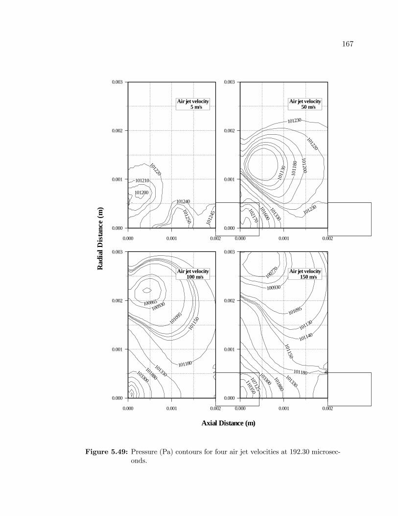
167

Axial Distance (m)

Rad

ialD

ista

nce

(m)

101210

101220

101250

101240

101200

1012

45

0.000 0.001 0.002

0.000

0.001

0.002

0.003

Airjet velocity5 m/s

101230

101220

101200

1011

80

1011

30

101230101600101330

102170

0.000 0.001 0.002

0.000

0.001

0.002

0.003

Airjet velocity50 m/s

101180

1011

501010

95

101330101880

103300

100865

100930

0.000 0.001 0.002

0.000

0.001

0.002

0.003

Airjet velocity100 m/s

101130

101095

100930

1007

70

101180101330

101880

103300110350

101150

101140

107125

0.000 0.001 0.002

0.000

0.001

0.002

0.003

Airjet velocity150 m/s

Figure 5.49: Pressure (Pa) contours for four air jet velocities at 192.30 microsec-onds.

168

Axial Distance (m)

Tur

bule

nce

Kin

etic

Ene

rgy

0

1200

2400

3600

4800

6000

Air jet velocity5 m/s

0

1200

2400

3600

4800

6000

Air jet velocity50 m/s

0

1200

2400

3600

4800

6000

Air jet velocity100 m/s

0.0000 0.0002 0.0004 0.0006 0.0008 0.0010 0.0012 0.0014 0.0016 0.0018 0.0020

0

1200

2400

3600

4800

6000

t = 15.38t = 23.07t = 76.92t = 192.30t = 376.92

microsec

Air jet velocity150 m/s

Figure 5.50: Temporal variation of turbulence kinetic energy of He-air mixturefor four air jet velocites along the jet symmetry axis at r = 0 m.

169

moves towards the transiently developing jet as the mean velocity of the steady jet

increases. The influence of streamline curvature on the turbulence kinetic energy

generation becomes evident when mean velocity of the steady jet exceeds 100 m/s.

In this case, turbulence kinetic energy generation becomes similar to that observed

for stagnation point flow [10]. Depending on the transiently developing jet profiles,

the magnitude of turbulence kinetic energy varies, i.e., the velocity profile resulting

in high streamline curvature effect gives rise to highest turbulence kinetic energy

generation, which occurs at 76.92 µs.

Figure 5.52 shows mass fraction of helium, nitrogen, and oxygen along the sym-

metry axis for different exiting mean velocity of the steady jet at 192.30 µs while

Figure 5.53 shows mass fraction of helium, nitrogen, and oxygen along the symmetry

axis for different times and 100 m/s mean velocity of the steady jet. Helium mass

fraction reduces gradually along the symmetry axis for low mean velocity of steady

jet. Moreover, increasing steady jet velocity results in sharp decay in helium mass

fraction. In the case of oxygen and nitrogen, sharp decay of mass fraction is observed

close to the transiently developing jet region. It should be noted that mass fraction

ratio of O2/N2 is 0.29 in the steady air jet. However, in the region close to the tran-

sient jet, this ratio changes and oxygen mass fraction increases. This indicates that

the diffusional transport of oxygen in the region close to the stagnation zone is higher

than that corresponds to nitrogen. This is more pronounced for high steady jet mean

velocities. Consequently, flow mixing and diffusional mass transport in the region

close to the stagnation zone modify the mass fraction of oxygen and nitrogen.

170

Axial Distance (m)

Axi

alV

eloc

ity(m

/s)

-150

-100

-50

0

50

100

150

Air jet velocity5 m/s

-150

-100

-50

0

50

100

150

Air jet velocity50 m/s

-150

-100

-50

0

50

100

150

Air jet velocity100 m/s

0.0000 0.0002 0.0004 0.0006 0.0008 0.0010 0.0012 0.0014 0.0016 0.0018 0.0020

-150

-100

-50

0

50

100

150

t = 15.38t = 23.07t = 76.92t = 192.30t = 376.92

microsecAir jet velocity150 m/s

Figure 5.51: Temporal variation of axial velocity of He-air mixture for four airjet velocites along the jet symmetry axis at r = 0 m.

171

Mas

sF

ract

ion

Axial Distance (m)

0.0

0.2

0.4

0.6

0.8

1.0

Air jet velocity50 m/s

0.0

0.2

0.4

0.6

0.8

1.0

Air jet velocity100 m/s

0.0000 0.0002 0.0004 0.0006 0.0008 0.0010 0.0012 0.0014 0.0016 0.0018 0.0020

0.0

0.2

0.4

0.6

0.8

1.0

HeliumNitrogenOxygen

microsec

Air jet velocity150 m/s

0.0

0.2

0.4

0.6

0.8

1.0

Air jet velocity5 m/s

Figure 5.52: Variation of mass fraction of helium, nitrogen and oxygen in He-airmixture for four air jet velocites along the jet symmetry axis at r =0 m and t = 192.30 microseconds.

172

Axial Distance (m)

Mas

sF

ract

ion

0.0000 0.0002 0.0004 0.0006 0.0008 0.0010 0.0012 0.0014 0.0016 0.0018 0.0020

0.0

0.2

0.4

0.6

0.8

1.0

t = 15.38t = 23.07t = 76.92t = 192.30t = 376.92

microsec

Oxygen

0.0

0.2

0.4

0.6

0.8

1.0

Nitrogen

0.0

0.2

0.4

0.6

0.8

1.0

Helium

Figure 5.53: Temporal variation of mass fraction of helium, nitrogen and oxygenin He-air mixture along the jet symmetry axis at r = 0 m and at airjet velocity of 100 m/s.

173

Table 5.1: Thermophysical properties of fluids used in the simulations.

Properties Air Helium (He) He−Air mixturek (W/m− k) 0.0242 0.152 0.0454cp (KJ/Kg −K) 1.006 5.193 1.000ρ (Kg/m3) 1.225 0.1625 −µ (Kg/m− s) 1.7894× 10−5 1.99× 10−5 1.72× 10−5M (Kg/Kgmol) 28.966 4.0026 28.966DAB (m

2/s) − − 2.88× 10−5

Chapter 6

CONCLUSIONS

6.1 Transient Jet Expansion into Stagnant Air

Transiently developing jet emanating from a free surface and expanding into air

ambient is considered to resemble the vapor jet behavior ejected from the laser-

produced cavity. Since the thermophysical properties of laser produced vapor is not

known, air or helium at 1500 K is considered as emerging jet in the simulations.

The jet exiting velocity profiles (jet velocity profiles onset of exiting the cavity) em-

ployed are obtained from the previous experimental study. This enables us to simulate

the actual laser produced cavity exiting conditions. A numerical scheme employing

control volume approach is employed when simulating the flow situations. The low

Reynolds number k − ε turbulence model is employed to account for the turbulence.

6.1.1 Transient Air Jet into Stagnant Air

It is found that in the early period the transient air jet expands more radially

than it does axially. As the time progresses, the jet width to jet penetration depth

ratio reduces. Once the jet exit velocity profiles become almost similar, self-similar

transient jet behavior is resulted. The specific conclusions derived from the present

174

175

study can be listed as follows:

1) Changes in jet exit velocity profiles result in variation in velocity magnitude

along the symmetry axis. This, in turn, alters the turbulence kinetic energy generation

in this region. Moreover, very small change in velocity magnitude results in large

change in turbulence kinetic energy.

2) In the early period temperature profiles follow the velocity profiles and the

convective heat transfer from the jet surface to its ambient is small. This occurs

because of small area of jet surface and short period of time, i.e., jet does not expand

enough to generate a large surface area and the period of expansion is short and hence

the heat transfer rate is low during early periods.

3) In the early period the ratio of jet expansion in the axial direction to the

one-fourth power of jet momentum rate per unit density increases linearly with the

square root of time, i.e., penetration number increases steadily. In this case, jet

behaves similar to those observed for slow flow jets. As time progresses, the rate of

momentum dissipation due to viscous dissipation becomes high and the penetration

number increases rapidly. This is observed for√t ≥ 12√µs in the present case.

6.1.2 Transient Helium Jet into Stagnant Air

It is found that the transient helium jet approaches self-similar behavior as the

dimensionless jet width (D/Zt) becomes 0.65 and the transition length of the jet is

obtained to be about 3 jet inlet diameters, which is less than the data reported in the

previous study. The specific conclusions derived from the present study are listed as

176

follows:

1) The flow entrainment results in a circulation cell in the region next to the jet

outer boundary after t = 76.92 µs. The orientation of circulation cell changes with

progressing time. This is due to the jet inlet velocity profiles, which varies with time.

2) Temperature contours follow almost the velocity profiles. Moreover, flow en-

trainment enhances the convective heat transfer rate, which in turn extends the high

temperature field into the jet-entrained region.

3) The mass ratio of helium decays sharply as the distance along the symmetry

axis increases away from the jet exit. The mixing of helium with air along the

symmetry axis indicates that while helium jet expands into the stagnant air, some

air molecules remain in the region close to the jet inlet as well as the expansion of

the helium into air accelerates the diffusional transport of air into helium jet.

4) In the early period of helium jet expansion, self-similar behavior of the jet is

not observed. This is because of the vast change of jet inlet velocity profiles in the

early period.

5) The constant penetration number

Ztµ •MHe/ρ

¶1/4×√t

is almost impossible dur-

ing the jet expansion in the present situation, since the jet inlet velocity changes

drastically in the early period.

6.2 Opposing Jets

The flow field due to opposing jet and transiently developing jet is studied in

relation to laser-induced ablation process. Steady jet represents the assisting gas

177

while transiently developing jet resembles the vapor plume emanating from the solid

surface during the ablation process. Since the thermophysical properties of the vapor

plume are not known, helium at 1500 K is employed for the transiently developing jet

while air is considered as an assisting gas. The flow, temperature and mass fraction

fields are simulated numerically using a control volume approach. The low Reynolds

number k − ε turbulence model is employed to account for the turbulence.

6.2.1 Transient Effect on The Flow Field Due to Opposing

Jets

It is found that the flow field in the region close to the transiently developing

jet is influenced considerably by the assisting gas jet. In the early stage transiently

developing jet expands in the axial direction and as the time progresses radial ex-

pansion of the jet dominates; in which case, a circulation cell next to the steady jet

boundary is developed. The specific conclusions derived from the present study can

be listed as follows:

1) The orientation and the size of the circulation cell next to the steady jet

boundary are influenced by the transiently developing jet entering velocities. In this

case, the velocity profile (similar to the profile for the fully developed flow) enhances

the size of the circulation cell.

2) The transiently developing jet influences the streamline curvature of the steady

impinging jet. In this case, enhancing radial flow suppresses the transiently developing

178

jet expansion in the axial direction.

3) The deep penetration of oxygen/nitrogen mass fraction into the region next

to the helium jet entry indicates that the flow mixing in this region occurs, i.e., next

to the stagnation region where two jets meet, the flow mixing is enhanced which can

also be observed through temperature contours. This is more pronounced as time

progresses.

4) A radial jet developed due to opposing of transiently developing and steady

jets. In this case, the radial jet show similar behavior to that corresponding to the

free jet, and the transiently developing jet characteristics do not affect considerably

the radial free jet characteristics.

5) The transiently developing jet does not approach a self-similar condition at

any period considered. Consequently, developing jet shows transient characteristics

for all the durations considered in the present study.

6) The penetration number of transiently developing jet attains almost steady

values during 10− 15√µs period. Moreover, sharp increase in penetration number in

the early period corresponds to the axial penetration of the jet.

6.2.2 Influence of Assisting Gas Velocity on The Flow Field

Due to Opposing Jets

It is found that the influence of the magnitude of the mean velocity of the steady

jet on the flow field in the region close to the transiently developing jet is found to be

179

very significant. In this case increasing mean velocity of impinging steady jet results

in development of the circulation cell next to steady jet boundary. The orientation

and strength of the circulation are modified by the mean velocity of the steady jet.

In this case, streamline curvature effect and flow entrainment cause flow mixing next

to the transiently developing jet boundary. Moreover, increasing mean velocity of the

steady jet suppresses the axial expansion of the transiently developing jet; hence, the

radial expansion of the jet is enhanced.

Mass fraction of helium decreases sharply in the axial direction as mean velocity

of the steady jet increases. Although the mass fraction ratio of O2/N2 in steady air

jet is 0.29 at jet inlet to the solution domain, it is modified in the region close to

the stagnation zone. In this case, oxygen mass fraction enhances in this region. This

suggests that flow mixing next to the transiently developing jet and diffusional mass

transport modify the mass fraction of species considerably in this region.

6.3 Future Work and Recommendations

Since laser-machining applications are involved with the laser non-conduction lim-

ited heating situation, phase change in the solid substrate should be considered when

modeling the laser-workpiece interaction. Moreover, the material properties vary with

temperature; therefore, temperature dependent properties should be accommodated

in the analysis. The rate of evaporation from the surface and the magnitude of recoil

pressure in the cavity determine the evaporating front velocity. Consequently, evapo-

rating front velocity of the vapor jet emanating from the cavity needs to be considered

180

when simulating the impinging gas effects on the laser-workpiece interaction.

Although the thermophysical properties of the evaporating front are not known,

a high-density gas, such as steam, can be introduced in the simulations to resemble

the evaporating front. The nucleation formation in the superheated liquid in the

cavity and droplet formation in the vapor phase during the plume expansion could

be accommodated in the heating model. Moreover, the influence of retarding zone on

the vapor front expansion could be included in the analysis.

Bibliography

[1] I. Sezai, and A.A. Mohamad, Three-Dimensional Simulation of Laminar Rect-angular Impinging Jets, Flow Structure, and Heat Transfer, ASME Journal ofHeat Transfer, Vol. 121, pp. 50-56, 1999.

[2] P.Y. Tzeng, C.Y. Soong, and C.D. Hsieh, Numerical Investigation of Heat Trans-fer under Confined Impinging Turbulent Slot Jets, Numerical Heat Transfer, PartA, Vol. 35, pp. 903-924, 1999.

[3] S.H. Seyedein, M. Hasan, and A.S. Mujumdar, Turbulent Flow and Heat Transferfrom Confined Multiple Impinging Slot Jets, Numerical Heat Transfer, Part A,Vol. 27, pp. 35-51, 1995.

[4] Y. Tzu, and C.H. Shyu, Numerical Study of Multiple Impinging Slot Jets withan Inclined Confinement Surface, Numerical Heat Transfer, Part A, Vol. 33, pp.23-37, 1998.

[5] H. Fujimoto, H. Takuda, N. Hatta, and R. Viskanta, Numerical Simulation ofTransient Cooling of a Hot Solid by an Impinging Free Surface Jet, NumericalHeat Transfer, Part A, Vol. 36, pp. 767-780, 1999.

[6] M.M. Rahman, A. J. Bula, and J.E. Leland, Conjugate Heat Transfer DuringFree Jet Impingement of a High Prandtl Number Fluid, Numerical Heat Transfer,Part B, Vol. 36, pp. 139-162, 1999.

181

182

[7] S.Z. Shuja, B.S. Yilbas, and M.O. Budair, Gas Jet Impingement on a SurfaceHaving a Limited Constant Heat Flux Area: Various Turbulence Models, Nu-merical Heat Transfer, Part A, Vol. 36, pp. 171-200, 1999.

[8] S.Z. Shuja, B.S. Yilbas, and M.O. Budair, Modeling of Laser Heating of SolidSubstance Including Assisting Gas Impingement, Numerical Heat Transfer, PartA, Vol. 33, pp. 315-339, 1998.

[9] T.J. Craft, L.J. W. Graham, and B.E. Launder, Impinging Jet Studies For Tur-bulence Model Assessment-II. An Examination of the Performance of Four Tur-bulence Models, International Journal of Heat and Mass Transfer, Vol. 36, No.10, pp. 2685-2697, 1993.

[10] D. Cooper, D.C. Jackson, B.E. Launder, and G.X. Liao, Impinging Jet Stud-ies For Turbulence Model Assessment-I. Flow-Field Experiments, InternationalJournal of Heat and Mass Transfer, Vol. 36, No. 10, pp. 2675-2684, 1993.

[11] S. Parneix, M. Behnia, and P.A. Durbin, Predictions of Turbulent Heat Transferin an Axisymmetric Jet Impinging on a Heated Pedestal, ASME Journal of HeatTransfer, Vol. 121, pp. 43-49, 1999.

[12] J.A. Fitzgerald, and S.V. Garimella, A Study of the Flow Field of a Confinedand Submerged Impinging Jet, International Journal of Heat and Mass Transfer,Vol. 41, No. 8-9, pp. 1025-1034, 1998.

[13] J.A. Fitzgerald, and S.V. Garimella, Flow Field Effects on Heat Transfer inConfined Jet Impingement, ASME Journal of Heat Transfer, Vol. 119, pp. 630-632, 1997.

[14] J. Sakakibara, K. Hishida, and M. Maeda, Vortex Structure and Heat Transfer inthe Stagnation Region of an Impinging Plane Jet (Simultaneous Measurementsof Velocity and Temperature Fields by Digital Particle Image Velocimetry andLaser-Induced Fluorescence), International Journal of Heat and Mass Transfer,Vol. 40, No. 13, pp. 3163-3176, 1997.

183

[15] Y.S. Chung, D.H. Lee, and J.S. Lee, Heat Transfer Characteristics of an Ax-isymmetric Jet Impinging on the Rib-Roughened Convex Surface, InternationalJournal of Heat and Mass Transfer, Vol. 42, pp. 2101—2110, 1999.

[16] H. Schlichting, Boundary Layer Theory, Seventh Edition, McGraw-Hill, NewYork.

[17] D.S. Lee, K.D. Kihm, and S.H. Chung, Analytical solutions for the developing jetfrom a fully- developed laminar tube flow, ASME Journal of Fluid Engineering,119, pp.716-718, 1997.

[18] R.V. Wilson and A.O. Demuren, Numerical Simulation of Turbulent Jets withRectangular Cross-Section, ASME Journal of Fluid Engineering, Vol. 120, pp.285-290, 1998.

[19] M.-H. Chen, and Z.-C. Hong, A pdf Description of Turbulent Axisymmetric FreeJet Flow, ASME Journal of Fluid Engineering, Vol. 121, pp. 73-79, 1999.

[20] J.C.F. Pereira, and J.M..P. Rocha, Numerical Computation of Convective Dis-persion in Turbulent Buoyant Jets, Numerical Heat Transfer, Part A, Vol. 23,pp. 399-414, 1993.

[21] G. Riopelle, G.D. Stubley, and A.B. Strong, Numerical Study of the Influence ofthe Ambient Pressure Field on Free Plane Turbulent Vertical Jets and Plumes,Numerical Heat Transfer, Part A, Vol. 26, pp. 273-286, 1994.

[22] G. Gerodimos, and R.M.C. So, Near-Wall Modeling of Plane Turbulent WallJets, ASME Journal of Fluid Engineering, Vol. 119, pp. 304-313, 1997.

[23] X. Zhou, Z. Sun, F. Durst and G. Brenner, Numerical Simulation of Turbulent JetFlow and Combustion, An International Journal of Computers & Mathematicswith Applications, Vol. 38, pp. 179-191, 1999.

[24] N.R. Panchapahesan, and J.L. Lumley, Turbulence Measurements in Axisym-

184

metric Jets of Air and Helium, Part 1, Air Jet, Journal of Fluid Mechanics, Vol.246, pp. 197-223, 1993.

[25] F.C. Lockwood, and H.A. Moneib, Fluctuating Temperature Measurements in aHeated Round Free Jet, Combustion, Science and Technology, Vol. 22, pp. 63-81,1980.

[26] X. Zhou, G. Brenner, T. Weber, and F. Durst, Finite-Rate Chemistry in Mod-elling of Two-Dimensional Jet Premixed CH4/Air Flame, International Journalof Heat and Mass Transfer, Vol. 42, pp. 1757-1773, 1999.

[27] Q.V. Nguyen, R.W. Dibble, C.D. Carter, G.J. Fiechtner, and R.S. Barlow,Raman-LIF Measurements of Temperature, Major Species, OH and NO inMethane-Air Bunsen Flame, Combustion and Flame, Vol. 105, pp. 449-510, 1996.

[28] X. Zhou, Z. Sun, G. Brenner, and F. Durst, Combustion Modelling of TurbulentJet Diffusion H2/Air Flame With Detailed Chemistry, International Journal ofHeat and Mass Transfer, Vol. 43, pp. 2075-2088, 2000.

[29] P. G. Hill, and P. Ouellette, Transient Turbulent Gaseous Fuel Jets for DieselEngines, ASME Journal of Fluid Engineering, Vol. 121, pp. 93-101, 1999.

[30] J.S. Turner, The Starting Plume in Neutral Surroundings, Journal of Fluid Me-chanics, Vol. 13, pp. 356-368, 1962.

[31] F.P. Ricou, and D.B. Spalding, Measurement of Entrainment by AsymmetricalTurbulent Jets, Journal of Fluid Mechanics, Vol. 11, Part 1, pp. 21-32, 1961.

[32] P. Ouellette, and P.G. Hill, Turbulent Transient Gas Injections, ASME Journalof Fluid Engineering, Vol. 122, pp. 743-753, 1999.

[33] J. Abraham, Entrainment Characteristics of Transient Gas Jets, Numerical HeatTransfer, Part A, Vol. 30, pp. 347-364, 1996.

185

[34] G. Singh, T. Sundararajan, and U.S.P. Shet, Entrainment and Mixing Studiesfor a Variable Density Confined Jet, Numerical Heat Transfer, Part A, Vol. 35,pp. 205-223, 1999.

[35] R.E. Breidenthal, The Turbulent Exponential Jet, Physics of Fluids, Vol. 29, No.8, pp. 2346-2347, 1986.

[36] X. Boyan, and M. Furuyama, Jet Characteristics of CNG Injector with MPISystem, JSAE Review, Vol. 19, pp. 229-234, 1998.

[37] J. Park, and H.D. Shin, Experimental Investigation of the Developing Process ofan Unsteady Diffusion Flame, Combustion and Flame, Vol. 110, 42, pp. 67—77,1997.

[38] K. Bremhorst, and P.G. Hollis, Velocity Field of an Axisymmetric Pulsed, Sub-sonic Air Jet, , AIAA Journal, Vol. 28, No. 12, pp. 2043-2049, 1990.

[39] J.S. Turner, Turbulent Entrainment: The Development of the Entrainment As-sumption, and its Application to Geophysical Flows, Journal of Fluid Mechanics,Vol. 173, pp. 431-471, 1986.

[40] F. Fang, and B.L. Sill, Experimental Investigation of Unsteady Submerged Ax-isymmetric Jets, Journal of Hydraulic Engineering, Vol. 113, No. 5, pp. 663-669,1987.

[41] H. Kouros, R. Medina, and H. Johari, Spreading Rate of an Unsteady TurbulentJet, AIAA Journal, Vol. 31, No. 8, pp. 1524-1526, 1993.

[42] H. Johari, Q. Zhang, M.J. Rose, and S.M. Bourque, Impulsively Started Turbu-lent Jets, AIAA Journal, Vol. 35, No. 4, pp. 657-662, 1997.

[43] G. Papadopoulos and W.M. Pitts, Scaling the Near-Field Centerline MixingBehavior of Axisymmetric Turbulent Jets, AIAA Journal, Vol. 36, No. 9, pp.1635-1642, 1998.

186

[44] G. Papadopoulos, and W.M. Pitts, A Generic Centerline Velocity Decay Curvefor Initially Turbulent Axisymmetric Jets, ASME Journal of Fluid Engineering,Vol. 121, pp. 80-85, 1999.

[45] J. Mi, and G.J. Nathan, Effect of Small Vortex-Generators on Scalar Mixing inthe Developing Region of a Turbulent Jet, International Journal of Heat andMass Transfer, Vol. 42, pp. 3919-3926, 1999.

[46] S. Aydore, and P.J. Disimile, Natural Coherent Structure Dynamics in NearField of Fully Turbulent Axisymmetric Jet, AIAA Journal, Vol. 35, No. 7, pp.1171-1178, 1997.

[47] H.B. Song, S. H. Yoon, and D. Hee, Flow and Heat Transfer Characteristics ofa Two-Dimensional Oblique Wall Attaching Offset Jet, International Journal ofHeat and Mass Transfer, Vol. 43, pp. 2395-2404, 2000.

[48] S.M. Hosseinalipour, and A.S. Mujumdar, Flow and Thermal Characteristics ofSteady Two-Dimensional Confined Laminar Opposing Jets: Part I. Equal Jets,Int. Comm. Heat Mass transfer, Vol. 24, No. 1, pp. 27-38, 1997.

[49] S.M. Hosseinalipour, and A.S. Mujumdar, Flow and Thermal Characteristics ofSteady Two-Dimensional Confined Laminar Opposing Jets: Part II. UnequalJets, Int. Comm. Heat Mass transfer, Vol. 24, No. 1, pp. 39-50, 1997.

[50] D.A. Johnson, Experimental and Numerical Examination of Confined LaminarOpposed Jets. Part I. Momentum Imbalance, Int. Comm. Heat Mass transfer,Vol. 27, No. 4, pp. 443-454, 2000.

[51] D.A. Johnson, Experimental and Numerical Examination of Confined LaminarOpposed Jets. Part II. Momentum Balancing, Int. Comm. Heat Mass transfer,Vol. 27, No. 4, pp. 455-463, 2000.

[52] S.M. Hosseinalipour, and A.S. Mujumdar, Comparative Evaluation of DifferentTurbulence Models for Confined Impinging and Opposing Jet Flows, NumericalHeat Transfer, Part A, Vol. 28, pp. 647-666, 1995.

187

[53] W.J. Sheu, and N.C. Liou, Efficiency of Heat Transfer Between Opposed Coro-tating Jets, Numerical Heat Transfer, Part A, Vol. 36, pp. 35-49, 1999.

[54] K.M. Lam, and H.C. Chan, Round Jet in Ambient Counter Flowing Stream,ASME Journal of Hydraulic Engineering, Vol. 123, No. 10, pp. 895-903, 1997.

[55] N. Benet, L. Falk, H. Muhr, and E. Plasari, Characterization and Modellingof a Two Impinging Jet Mixer for Precipitation Process Using Laser InducedFluorescence, 10 th European conference on mixing, pp. 35-44, 2000.

[56] P.O. Witze, and H.A. Dwyer, The Turbulent Radial Jet, Journal of Fluid Me-chanics, Vol. 75, No. 3, pp. 401-417, 1976.

[57] M.A. Jarrah, T.K. Aldoss, and A.M. Al-Sarkhi, Interaction of Two OppositeConical Curved Wall Jets, International Journal of Heat and Fluid Flow, Vol.17, No. 4, pp. 397-402, 1996.

[58] J.N. Gonsalves, and W.W. Duley, Cutting Thin Metal Sheets with the CW CO2laser, Journal of Applied Physics, Vol. 43, No. 11, pp. 4684-4687, 1972.

[59] M.F. Modest, and H. Abakians, Evaporative Cutting of a Semi-Infinite bodywith Moving CW Laser, Journal of Heat Transfer, Vol. 108, pp. 602-607, 1986.

[60] S.Y. Bang, and M.F. Modest, Multiple Reflection Effects on Evaporative CuttingWith a Moving CW Laser, Journal of Heat Transfer, Vol. 113, pp. 663-669, 1991.

[61] S. Roy, and M.F. Modest, CW Laser Machining of Hard Ceramics-I, Effects ofThree-Dimensional Conduction, Variable Properties and Various Laser Param-eters, International Journal of Heat and Mass Transfer, Vol. 36, No. 14, pp.3515-3528, 1993.

[62] S.Y. Bang, S. Roy, and M.F. Modest, CW Laser Machining of Hard Ceramics-II,Effects of Multiple Reflections, International Journal of Heat and Mass Transfer,Vol. 36, No. 14, pp. 3529-3540, 1993.

188

[63] M.F. Modest, Three-Dimensional, Transient Model for Laser Machining of Ablat-ing/Decomposing Materials, International Journal of Heat and Mass Transfer,Vol. 39, No. 2, pp. 221-234, 1996.

[64] M.F. Modest, Laser Through-Cutting and Drilling Models For Ablat-ing/Decomposing Materials, Journal of Laser Applications, Vol. 9, pp. 137-145,1997.

[65] B.S. Yilbas, and Z. Yilbas, Some Aspects of Laser-Metal Vapor Interaction,Pramana–Journal of Physics, Vol. 31, No. 5, pp. 365-381, 1988.

[66] B.S. Yilbas, R. Davies, Z. Yilbas and A. Koc, Analysis of the Absorption Mech-anism During Laser-Metal Interaction, Pramana–Journal of Physics, Vol. 34,No. 6, pp. 473-489, 1990.

[67] P.S. Wei, and J.Y. Ho, Energy Considerations in High-Energy Beam Drilling,International Journal of Heat and Mass Transfer, Vol. 33, No. 10, pp. 2207-2217, 1990.

[68] R.K. Ganesh, A. Faghri, and Y. Hahn, A Generalized Thermal Modelling forLaser Drilling Process–I. Mathematical Modeling and Numerical Methodology,International Journal of Heat and Mass Transfer, Vol. 40, No. 14, pp. 3351-3360,1997.

[69] R.K. Ganesh, A. Faghri, and Y. Hahn, A Generalized Thermal Modelling forLaser Drilling Process–II Numerical Simulation and Results, International Jour-nal of Heat and Mass Transfer, Vol. 40, No. 14, pp. 3361-3373, 1997.

[70] Y. Zhang, and A. Faghri, Vaporization, Melting, and Heat Conduction in theLaser Drilling Process, International Journal of Heat and Mass Transfer, Vol.42, pp. 1775-1790, 1999.

[71] A.V. Gusarov, A.G. Gnedovets, and I. Smurov, Two-Dimensional Gas-DynamicModel of Laser Ablation in an Ambient Gas, Applied Surface Science, Vol. 154-155, pp. 66-72, 2000.

189

[72] A. Kar, J.A. Rothenflue, and W.P. Latham, Scaling Laws for Thick-SectionCutting With a Chemical Oxygen-Iodine Laser, Journal of Laser Applications,Vol. 9, pp. 279-286, 1997.

[73] V. Semak, and A. Matsunawa, The Role of Recoil Pressure in Energy BalanceDuring Laser Materials Processing, J. Phys. D: Appl. Phys., Vol. 30, pp. 2541-2552, 1997.

[74] D.C. Wilcox, Turbulence Modeling for CFD, chapter 5, pp. 223-252, DCW In-dustries Inc., 2000.

[75] H.K. Versteeg, and W. Malalasekera, An Introduction to Computational FluidDynamics, The Finite Volume Method, Longman Scientific and Technical, 1995.

[76] W. Rodi, Turbulence Models and Their Application in Hydraulics–A State ofthe Art Review, Presented by the IAHR-Section on Fundamentals of Division II:Experimental and Mathematical Fluid Dynamics, 1984.

[77] C.K.G. Lam, and K.A. Bremhorst, Modified Form of the K − ² Model for Pre-dicting Wall Turbulence, Trans. ASME, Journal of Fluid Engineering, Vol. 103,pp. 456-460, 1981.

[78] B.S. Yilbas, G.M. Arshed, and H.I. Acar, Investigation into Laser ProducedEvaporating Front Characteristics in Relation to Laser Drilling, Lasers in Engg.,Vol. 13, pp. 65-74, 2003.

[79] R.S. Amano, and H. Brandt, Numerical Study of Turbulent Axisymmetric JetsImpinging on a Flat Plate and Flowing into an Axisymmetric Cavity, ASMEJournal of Fluid Engineering, Vol. 106, pp. 410-417, 1984.

[80] B.E. Launder, and D.B. Spalding,Mathematical Models of Turbulence, AcademicPress Inc. (London) Ltd., Third Printing 1979.

[81] S.V. Patankar, Numerical Heat Transfer and Fluid Flow, Series in Computa-

190

tional Methods in Mechanics and Thermal Sciences, McGraw-Hill Book Com-pany, 1980.

[82] B.S. Yilbas, S.Z. Shuja, and M.O. Budair, Stagnation Point Flow Over a HeatedPlate: Consideration of Gas Jet Velocity Profiles, in Print, AJSE, pp. xx-xx,2003.

[83] I. Wygananski, and H. Fielder, Some Measurements in the Self-Preserving Jet,Journal of Fluid Mechanics, Vol. 38, Part 3, pp. 577-612, 1969.

[84] P.O. Witze, The Impulsively Started Incompressible Turbulent Jet, Sandia Lab-oratories Report SAND80-8617, Livermore, California, 1980.

[85] R.D. Blevins, Applied Fluid Dynamics Handbook, Van Nostrand Reinhold Com-pany, 1984.

VITA

Ghulam Murshed Arshed

• Born: in Karachi, Pakistan.

Address: 2/2, sector # 23, Reta Plot, Drigh Colony, Karachi−75230, Pakistan.

Phone: (92-21) 457-8337

(92-21) 501-8916

• Received Bachelor of Engineering from NED University of Engineering and

Technology (Mechanical engineering) Karachi, Pakistan, 1995.

• Joined Mechanical Engineering Department of King Fahd University of

Petroleum and Minerals, Dhahran, as a Research Assistant in 2000.

• Finished Master of Science in Mechanical Engineering from King Fahd Univer-

sity of Petroleum and Minerals, Dhahran, Saudi Arabia, 2003.

191