© Jones & Bartlett Learning, LLC The Science of © Jones ...

© W

eiming

Che

n/Ge

tty Im

ages

The Science of Environmental HealthLEARNING OBJECTIVESAfter studying this chapter, the reader will be able to:

• Define or explain the key terms and concepts introduced throughout the chapter and summarized in Table 2.1• Explain key features of both the atmosphere and hydrologic cycle and explain how these features relate to the distribution of pollutants within the Earth’s air and water supply• Describe how the characteristics of individual chemicals affect their fate and transport in the environment• Distinguish the key scientific and methodologic domains of environmental health and how they relate to one another• Present a conceptual model of toxicologic exposure, identifying key events and processes as well as estimates of effects; distinguish between routes and pathways of exposure; and explain the standard units of absorbed dose• Explain the distinction between descriptive and analytic epidemiologic study designs, compare and contrast the key measures used in surveillance, and discuss criteria for concluding that an association represents a causal connection• Describe the major steps in a risk assessment for the noncancer and carcinogenic effects of environmental hazards

In this chapter, we describe the science and research methods that enhance our understand-ing of environmental pollutants and the hazards they pose to people.

• After discussing atmospheric and aqueous characteristics and terms in Section 2.1, we learn about the behavior of contaminants—their chemical or physical transformations, and their movements with or between envi-ronmental media, such as air and water. Taken together, these events are commonly

referred to as the fate and transport of contaminants in the environment.

• Section 2.2 presents the principles of toxicology, the science of the adverse effects of toxic agents—chemicals, includ-ing natural toxins, and also physical haz-ards such as asbestos fibers or radiation—on normal biological structure and function in humans and other living things. In a sense, toxicology continues the story of the fate and transport of environmental contaminants

7

CHAPTER 2

© Jones & Bartlett Learning LLC, an Ascend Learning Company. NOT FOR SALE OR DISTRIBUTION.

© Jones & Bartlett Learning, LLCNOT FOR SALE OR DISTRIBUTION




















Table 2.1 Significant Terms and Concepts

Fate and transport Toxicology Exposure assessment

Epidemiology Risk assessment Limiting factor

Greenhouse effect Ozone layer Temperature inversion

Gyre Thermohaline circulation Surface water

Aquifer vadose or unsaturated zone Saturated zone

Leachate Lipophilic Bioconcentration

Bioaccumulation Xenobiotic Biomagnification

Persistence Toxicokinetics Toxicodynamics

Epigenetics Teratogenesis Dose-response

Slope Threshold LD50

NOAEL LOAEL Biomarkers

Morbidity Prevalence Incidence

DALY Surveillance Confounding

Rate adjustment Ecological fallacy Cross-sectional study

Relative risk, RR Cohort study Case-control study

Odds ratio Bias Deterministic risk

Stochastic risk Reference Dose, RfD Hazard Quotient, HQ

Cancer slope factor, CSF

into the interior realm, studying their move-ments, transformations, and ultimate effects in the body.

• The applied science of exposure assessment is presented in Section 2.3, providing the methods used to measure or estimate human contact with environmental contami-nants. Exposure can be assessed both outside and inside the body, and so exposure assess-ment not only draws on an understanding of the processes of environmental fate and trans-port but also on insights from toxicology.

• Section 2.4 describes aspects of epidemiology that provide insight into how envi-ronmental hazards have directly affected humans. By using specialized quantitative methods and drawing on exposure assess-ment science, epidemiologic observations

may suggest connections between environ-mental hazards and health effects before the scientific mechanism is understood.

• The chapter concludes with Section 2.5 describing risk assessment as the set of formal procedures for evaluating and inte-grating scientific information on exposure and toxicity in order to quantify the real-world public health risk of a hazard. Risk assessment is broadly integrative, bringing together information from environmental science, toxicology, exposure assessment, and epidemiology. In environmental health, the formal risk assessment approach is applied mostly to toxicants such as chemicals, partic-ulates, and radiation; however, its influence can also be seen in the evaluation of patho-genic hazards.

8 Chapter 2 The Science of Environmental Health






















2.1 Pollution on Our Planet

The story of human exposure to environmental contaminants begins with the fate and trans-port of these agents—their transformations and movements—through the atmosphere or an aque-ous environment.

The AtmosphereThe Earth’s atmosphere, although it may seem formless, has a clear structure and regular pat-terns of movement.

Layers of the AtmosphereThe innermost layer of the Earth’s atmosphere, called the troposphere, extends to an altitude of approximately 8 miles (13 kilometers); within the troposphere, temperature declines with increasing altitude. Most of what we experience as weather takes place in the troposphere.

Air in the troposphere is made up mostly of two colorless, odorless gases: by volume, about 78% nitrogen (N

2) and 21% oxygen (O

2). Human

life on this planet is possible because of oxygen, described in ecological terms as a limiting factor, a resource required for survival. The concentra-tion of O

2 decreases in the upper regions of the

troposphere to levels unsustainable for humans, even at elevation levels for some of our highest mountain peaks. Of the remaining components in the atmosphere, known as trace gases, the most abundant by volume is argon, which is chemically inert; that is, under ordinary conditions, it does not react with other substances. Other trace gases are more important to life on Earth and to public health: In particular, water vapor (H

2O), carbon

dioxide (CO2), methane (CH

4), nitrous oxide

(N2O), and ozone (O

3) all function as greenhouse

gases. As the Earth radiates heat energy that it has absorbed from sunlight, greenhouse gases in the troposphere absorb some of that heat and reradi-ate it back toward the Earth’s surface. This return of energy—a natural greenhouse effect—keeps the Earth’s climate warm enough to support life (see Figure 2.1).

Above the troposphere lies the strato-sphere, reaching to an altitude of about 30 miles (48 kilometers). Within the stratosphere, tem-perature rises with increasing altitude. Roughly in the middle of the stratosphere is a layer in which the concentration of ozone is much higher than at other altitudes within the stratosphere. This stratospheric ozone layer absorbs much of the incoming ultraviolet radiation from the sun; without this protection, human beings could not live on Earth. (Ozone formed in the troposphere from anthropogenic pollutants, on the other hand, has negative effects on respiratory health, as described later in the context of burning fossil fuels to produce energy.)

Beyond the stratosphere lie the two outer layers of the atmosphere: the mesosphere and the thermosphere. The atmosphere does not have a sharply defined boundary at its outer edge but rather gradually becomes thinner and disappears.

Global and Local Patterns of Air CirculationOn a global scale, prevailing winds at the Earth’s surface are easterly in the equatorial region—these are the trade winds, so named because they carried sailing ships on trade routes from Europe to the Americas. In the midlatitudes, both north and south, westerly winds prevail; in the polar regions, easterly winds again pre-vail. These wind patterns result from the com-bined effects of two processes—the Earth’s rotation and vertical air circulation driven by temperature gradients—and can carry air pol-lutants over long distances, spreading them both horizontally and vertically.

Regular wind patterns also operate on smaller scales. For example, many coastal locations, where the land heats and cools more rapidly than the adjacent water each day, experience onshore winds during the daytime and nighttime winds that blow out to sea.

More generally, local and regional weather conditions affect the degree of horizontal and vertical mixing of air, and, therefore, the dis-persion of pollutants in the air. Such disper-sion may actually be visible near a source—for

2.1 Pollution on Our Planet 9






















example, in the form of a plume of smoke trail-ing from a smokestack, becoming broader and less concentrated with increasing distance from the source.

Sometimes, local weather prevents such dilution of air pollutant concentrations and in extreme cases can turn that pollution into an immediate public health threat. The extreme case of such conditions is a temperature inversion, in which a mass of cooler, heavier air becomes trapped at ground level—often in a valley—beneath a layer of warmer, less-dense air. Under this “ceiling,” little mixing occurs, and emissions from local sources can accumulate, causing pol-lutants to reach dangerously high concentrations.

Air pollution comes from either natural or anthropogenic sources. Dust storms, salt evapora-tion, forest fires, volcanos, mold spores and plant materials, such as pollen, all introduce poten-tially hazardous pollutants derived from natu-ral sources. Anthropogenic sources are further

categorized as either stationary or mobile sources. Emissions from smokestacks, like what is depicted in Figure 2.2, are a type of stationary source, and such emissions are part of many indus-trial processes, such as electricity generation, oil refineries, or incinerators. Mobile anthropogenic sources refer to on- and off-road vehicles, as well as airplanes, ships, and trains, which introduce pollution through combustion engines and their associated “tail-pipe” emissions.

Water in the Ambient EnvironmentLike the atmosphere, the Earth’s water can trans-port pollutants at global and local scales, in ways both visible and invisible.

The Global Hydrologic CycleThe Earth’s water is connected via a complex web of processes, presented in simplified form in

Figure 2.1 The atmosphere.

Troposphere78% N21% O2Remainder-Argon andgreenhouse gases

Occan

MountainsEarth

Stratosphere

Ozone layer























Figure 2.3. Not all aspects of this hydrologic cycle are readily apparent: Although oceans, lakes, and rivers are prominent features of the sur-face environment, both underground water and water vapor are largely invisible.

As shown in Figure 2.3, evaporation and pre-cipitation create a continuous exchange of water between the atmosphere and the Earth’s surface. The majority of this exchange occurs between the atmosphere and the ocean. Furthermore, the bal-ance of precipitation and evaporation is different on land and sea: The oceans experience a net loss of water through these processes, while land areas experience a net gain. Most of the excess water from precipitation onto land returns to the oceans via rivers; a much smaller volume returns via groundwater.

Ocean WatersOcean currents play an integral role in moderating the Earth’s climate, and they also create underwater “climates” supporting populations of fish on which humans depend for food. And, like prevailing

winds, ocean currents can carry pollutants for long distances. In January of 1992, a ship en route from Hong Kong to Tacoma, Washington, lost several containers of plastic bath toys overboard during a storm, including 7,200 yellow plastic ducks. The incident occurred near the International Date Line in the Northern Pacific Ocean, south of the Aleutian Islands that extend westward from Alaska. Over the next few years, plastic ducks were recov-ered at Shemya Island, near the western tip of the Aleutians, at several points along the coast of the Alaska panhandle, and on the Washington and Oregon coasts. In 2003, one well-weathered duck turned up near Kennebunkport, Maine, probably having spun off westward in the Pacific and trav-eled around the globe.1

In oceanology, any large system of circulat-ing ocean currents is termed a gyre and there are 11 major gyres described in the world’s oceans. The accumulation of marine debris, particularly plastic, has become more of a major concern associated with subtropical gyres than a bunch of floating rubber ducks. Large garbage patches form in eddy-like areas within these gyre circulation

Figure 2.2 Stationary sources of air pollution.























patterns where debris stalls and creates large masses.2 Although much of the plastic accumu-lates, these patches also serve as a source for the release of plastic breakdown products for centu-ries to come (refer to Figure 2.4)

The oceans’ major surface currents are driven by friction between air and water and so mimic the global prevailing winds: easterly near the equa-tor and westerly in the midlatitudes. But unlike the winds, these major ocean currents are further deflected by the continents so that they form large rotating cells, flowing clockwise north of the equa-tor and counterclockwise south of the equator. Deeper ocean waters also circulate along predict-able paths, moving more slowly than surface waters and looping through all of the world’s oceans like a continuous conveyor belt. This process is largely independent of the surface currents, being driven mainly by differences in the density of the water related to temperature and salinity and, therefore, known as the thermohaline circulation. The global thermohaline circulation is propelled by events in the North Atlantic. Here, deeper seawa-ter is northbound along the European coast. The northbound water quickly becomes both colder

and saltier (because salt is excluded from ice that is being formed). Both of these changes make the seawater denser, and as a result, it drops suddenly to the ocean floor. This event drives the beginning of a new global circuit by the deep ocean waters influencing how marine pollution is distributed.

Fresh WaterAlthough the earth’s surface is covered largely by water, all but 3% of the planet’s water resources are nonpotable ocean water. Humans rely on freshwater for survival, and more than half of all freshwater is unavailable frozen in icecaps and glaciers. Of the remaining freshwater, less than 1% is readily accessible from surface water sources, such as lakes and rivers.3 Typically, a river begins as a set of small streams that converge in stepwise fashion, ultimately uniting as a river. The area drained by a river and the streams that feed it is referred to as the river’s drainage basin. Some surface water systems span very large geographic regions; for example, the drainage basin of the Amazon River, with all of its tributaries, extends throughout Brazil.

Uptakeby roots

Transpirationby leaves

Evaporation

EvaporationEvaporation

Condensationand precipitation



Waterheld inplants

Ocean Rivers,lakes

Streamflow(on the surface)

Groundwater flow(underground)

Groundwater flow(underground)

Water vaporin atmosphere

Liquid water Water vaporKey:

Groundwater

Figure 2.3 Hydrologic cycle.























Surface water sources of pollution are char-acterized as either point or nonpoint pollution, an apt description since one may literally point to the pollution discharged from industrial or municipal pipes, representing either chemical or biological contamination. Nonpoint sources of water pollution consist of runoff from roads, agricultural activities and construction, sewage overflows, and atmospheric deposition, and can also be chemical or biologic in origin.

Less visible than surface water, and far less familiar to most people, is the water located under-ground (see the conceptual model in Figure 2.3 and a more comprehensive depiction in Figure 2.5). Underground sources of fresh water reside in aquifers, geologic material that is porous enough to hold and transmit water through the pore spaces between the geologic material. Aquifers are most often sand or gravel but can be porous rock such as sandstone, or even fractured rock, and they are typically covered by surface soil.

As precipitation soaks into the ground, water moves downward through pore spaces. In the topmost subsurface zone, water may also evapo-rate or transpire to the atmosphere. Transpiration is a process through which water taken up by

the roots of plants is released to the atmosphere through their leaves. Whenever more water enters the topmost zone from precipitation than leaves via evaporation and transpiration, the water moves farther downward.

The area above the water table is called the vadose or unsaturated zone. In this zone, the pore spaces are partly filled by water. Water that trickles downward through the vadose zone recharges the aquifer—that is, feeds or replenishes it.

Below the vadose zone is the saturated zone, in which all pore spaces are filled with water. In the saturated zone, groundwater seeps slowly in response to gradients of elevation and pressure toward a location where water is dis-charged continuously—for example, via a spring. In most locations, groundwater flows at a rate of only centimeters or inches per day. When speaking of groundwater flow, the term downgra-dient is used in place of downstream.

The area on the ground surface through which rainfall feeds an aquifer is called the aquifer’s recharge area. The lower limit of the aquifer (the floor) is an underlying layer of rock or clay that is impermeable, or nearly so. In a simple geologic

Figure 2.4 Plastic garbage patch.National Oceanic and Atmospheric Administration. https://oceanservice.noaa.gov/facts/garbagepatch.html























setting like the one just described, the recharge area is directly above the aquifer, with no intervening impermeable layer. This is called an unconfined aquifer or water table aquifer. The surface of the water table often follows, in muted fashion, the contours of the land surface above. (In fact, con-tour lines are used to represent the water table sur-face in maps, much as they are used to represent differences in surface elevation.) If a well is drilled into a water table aquifer—leaving a cylinder made of a fine mesh so that water can flow into the borehole—the water level in the well will be the same as that in the surrounding aquifer.

Wastes or other products placed in the ground or on the Earth’s surface within the recharge area of a water table aquifer can con-taminate the aquifer. For example, if a chemical such as trichloroethylene is spilled on the ground surface, or dumped into a pit, it can trickle down to the water table. The contamination will then

take the form of a plume as the chemical is carried along slowly with the groundwater, gradually dis-persing horizontally and vertically—not unlike an airborne plume of smoke. A well that draws water from within such a plume will produce contami-nated water.

Similarly, rainwater percolating downward through wastes placed on the ground surface (or in a pit) can dissolve out or suspend contaminants and carry them along, much as water poured through ground coffee beans dissolves out of the substances that make the water into coffee. Water that has been contaminated by such leaching of contaminants is known as leachate.

An aquifer that is sandwiched between lay-ers of impermeable (or nearly impermeable) rock is known as a confined aquifer. Largely isolated from local precipitation, confined aqui-fers are replenished very slowly and are often considered a finite resource in terms of human

Figure 2.5 Groundwater features.Special thanks to Ronald W. Falta, Jr.

Waterwell

Unsaturated (vadose) zone

Water table

Saturated zone (unconfined aquifer)

Confining layer (does not transmit water easily)

Water filledConfined aquifer























lifespans. Today’s aquifers were formed long ago and bear the imprint of their geologic histories. In many geologic settings, layers of water-bearing rock alternate with impermeable layers so that aquifers are stacked beneath the Earth’s surface. Aquifers vary widely in geographic scale. For example, some 25 aquifers are recognized within Massachusetts; in contrast, the extensive Ogallala Aquifer underlies parts of eight U.S. states from South Dakota to Texas. Once a confined aquifer has been contaminated, from underground stor-age tanks or purposeful deep-well injection, such as that associated with hazardous waste disposal, it is very difficult and expensive to clean up.

The Fate and Transport of Environmental ContaminantsEnvironmental contaminants in the ambient environment can be found in air, water, or soil, including soil that is dry and fine enough to

become airborne (dust) and soil in bodies of water ( sediment). The preceding descriptions of air and water movement in the ambient envi-ronment were presented because pollutants are basically passengers along for a ride through the environmental media. However, they are, in a sense, passengers with preferences based on their chemical, biological, or physical properties.

Physical–Chemical Properties of ChemicalsContaminants have characteristics, known as physical–chemical properties, which affect their behavior in the environment (see Figure 2.6). For example, the fate of a liquid chemical spilled on the ground depends partly on its volatility (a): the tendency to change into gaseous form (to volatilize). In the environment, a highly vol-atile liquid chemical that is spilled will move rapidly into a gaseous form that cannot easily be cleaned up. Similarly, aqueous solubility (b) is

Chemicalin air

Solubility (b)Lipophilic

tendency (e)

Volatility (a) Partitioningwater/air (c)

Partitioningwater/carbon (d)

Chemical insoil/sediment

containingorganic carbon

Chemicalin liquid

form

Chemicalin water

Chemical inliving tissue(e.g., fish)

Figure 2.6 Physical-chemical properties of chemicals.























the tendency of a chemical to dissolve in water; a highly water-soluble chemical spilled into a lake is likely to become widely dispersed in the water. ( Aqueous solubility is often referred to simply as solubility.)

A third property—a chemical’s affinity for water versus air (c)—reflects whether the chem-ical is more soluble than volatile, or vice versa. In conceptual terms, such an affinity represents the division, or partitioning, of the chemical between water and air that would occur if the process reached a state of equilibrium. In practice, the shift toward such an equilibrium state in the envi-ronment may be rapid or slow.

Chemicals also show an affinity for soil or sediment—actually, the organic carbon in soil or sediment—versus water (d). Chemicals with a high affinity for organic carbon tend to cling to the sed-iments of a stream, for example, rather than being found in the water. Finally, chemicals vary in their tendency to move from water to an oily medium (e). Chemicals having such a tendency are called lipophilic (fat-loving) or fat-soluble. Lipophilic chemicals in lakes or streams tend to move into the fatty tissues of aquatic organisms, or biocon-centrate; bioconcentration is a biological con-sequence of these chemicals’ lipophilic tendency.*

A chemical that tends to bioconcentrate poses a potential threat to organisms through two fur-ther processes. Bioaccumulation is the build-ing up of a chemical in an individual organism’s tissues over its lifetime as the organism continues to take in more than it excretes. Environmental pollutants that share similar characteristics, such as chemical shape or lipophilic tendencies, to those of human substances are considered xenobiotics (xeno means foreign), and the loca-tion where these foreign chemicals bioaccumulate may be predicted based on the human substance they resemble. For example, a biotransformed chemical product of polychlorinated biphenyls (PCBs) closely resembles the chemical structure

* Some chemicals, including methylmercury, are not highly lipophilic but do concentrate in the muscle tissue of animals.

of thyroxine, human growth hormone, and may fool the body into storing it within its fat cells.4

Biomagnification is a different process by which a chemical becomes more concentrated in the tissues of organisms at each higher trophic level in a food chain; for example, in big fish that eat smaller fish, and in eagles (or people) that eat the big fish. In contrast to bioconcentra-tion, bioaccumulation and biomagnification are not just properties of individual chemicals but rather processes that take place in organisms and ecosystems.

In practical terms, groups of chemicals with similar properties show similar environmental tendencies. For example, low–molecular-weight solvents such as trichloroethylene and benzene are highly volatile and moderately soluble; they are very likely to become air contaminants but unlikely to cling to soil. At the other extreme, very heavy chemicals such as PCBs and dioxins have very low solubility and volatility; they are unlikely to be air or water contaminants, but rather are found in soil or sediment as well as reside in fat. Chemicals’ behavior can also be affected by environmental conditions; for example, a volatile chemical moves from a liquid to a gaseous state more rapidly in warmer weather.

Finally, a chemical in the environment does not persist indefinitely as the same chemical but rather is transformed into other chemicals. A chemical’s persistence in the environment is often quantified as its half-life in air, water, or soil. The environmental half-life of a chemical in a given medium is the period of time after which one-half of the original quantity is expected to have been chemically or biologically transformed. The term half-life is borrowed from radioac-tive decay; however, unlike radioactive half-life, the environmental half-life of a chemical is only approximate because it is greatly affected by envi-ronmental conditions, such as the presence of light or oxygen. The half-life of the pesticide DDT in soil, for example, ranges from about 8 to 15 years. In general, chemicals of higher molecular weight tend to be more persistent. The environmental persistence in soil or sediment of high-molecular- weight, lipophilic contaminants such as DDT or dioxin presents the opportunity for long-term























exposures and thus greater potential for bioaccu-mulation and biomagnification. Even persistent chemicals, however, do not persist indefinitely in the environment, but gradually break down.

2.2 Toxicology: The Science of Poisons

The term environment suggests something that merely surrounds us, but we are more perme-able than we like to think. People contact—and absorb—environmental contaminants mainly by three major routes of exposure: inhalation (mostly through ordinary continuous breathing), ingestion (by eating and drinking), and dermal contact (via the skin). Toxicology is the study of how the body processes the toxicants to which it is exposed and of the ultimate effects of these toxicants in the body.

In toxicology, the term toxin is reserved for a naturally produced toxic substance, especially one produced by a plant or animal. The term tox-icant usually refers to toxic substances that result from human activities, although this definition is stretched to include such naturally occurring agents as toxic metals (e.g., arsenic) or radiation, which are not produced by a plant or animal. In this text, the term toxicant is used except when referring specifically to natural plant or animal toxins.

The Disposition of Chemicals in the BodyWhatever the route of exposure, a chemical is absorbed into the body by passing through cell membranes. From the exposure perspective, the linings of the lungs and digestive tract may be thought of as part of the boundary between the external and internal environments—in effect, as extensions of the skin. In fact, absorption via inhalation and ingestion is much more rapid and complete than dermal absorption because the lungs and digestive tract are designed to absorb oxygen and nutrients, whereas the skin is funda-mentally a protective barrier.

Exposure to environmental toxicants is often defined as contact with the human envelope, and the

human envelope is defined in turn as the boundary that separates the interior of the human body from the exterior environment. Exposure is quantified as a dose, and absorbed dose refers specifically to the amount of some toxicant that passes through the human envelope, entering the body.

After being absorbed, chemicals are distrib-uted around the body via the bloodstream or the lymph system, and may be metabolized (chemi-cally transformed by enzymes) during the course of this journey. Much, though not all, metabolism of chemicals takes place in the liver. The pro-cesses of distribution and metabolism interact: A chemical’s path through the circulatory system affects how it is metabolized, and how and where it is metabolized determines its chemical form, which in turn affects whether, and how, it is stored or excreted. These processes are shown in sim-plified form in Figure 2.7. The term metabolite refers to a product of the body’s metabolism of a toxicant or toxin.

Lipophilic contaminants, including some pes-ticides, are stored in fat cells, and lead is deposited in bone (where it substitutes for calcium). How-ever, excretion, by removing some quantity of a toxicant from circulation, can allow some of the same toxicant to be released from storage. Chem-icals are not only excreted from the body, mostly in exhaled air, urine, and feces but also in sweat and semen and by deposition in hair and nails, which in this context are seen as being outside of the human envelope. (This is why it doesn’t hurt to cut your hair or nails.) Breast milk may also be a route of excretion; from the perspective of the infant, of course, breast milk becomes a source of ingestion exposure.

The combined processes of absorption, dis-tribution, metabolism, storage, and excretion of toxicants are collectively referred to as toxicokinetics and determine the disposition of a chemical in the body. The net effect of these processes is reflected in the total burden of the chemical, or of some breakdown product, pres-ent in the body at some point in time (the body burden). Of more interest in toxicology, how-ever, is the biologically effective dose: The quantity of a toxicant or its breakdown product

2.2 Toxicology: The Science of Poisons 17






















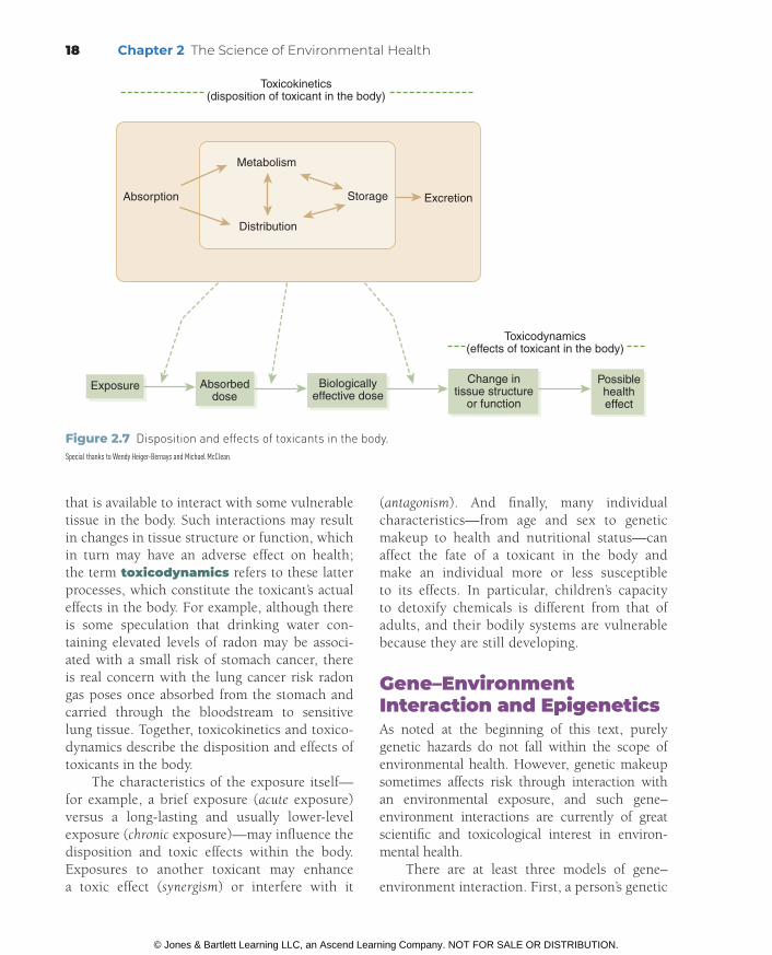
that is available to interact with some vulnerable tissue in the body. Such interactions may result in changes in tissue structure or function, which in turn may have an adverse effect on health; the term toxicodynamics refers to these latter processes, which constitute the toxicant’s actual effects in the body. For example, although there is some speculation that drinking water con-taining elevated levels of radon may be associ-ated with a small risk of stomach cancer, there is real concern with the lung cancer risk radon gas poses once absorbed from the stomach and carried through the bloodstream to sensitive lung tissue. Together, toxicokinetics and toxico-dynamics describe the disposition and effects of toxicants in the body.

The characteristics of the exposure itself—for example, a brief exposure (acute exposure) versus a long-lasting and usually lower-level exposure (chronic exposure)—may influence the disposition and toxic effects within the body. Exposures to another toxicant may enhance a toxic effect (synergism) or interfere with it

(antagonism). And finally, many individual charact eristics—from age and sex to genetic makeup to health and nutritional status—can affect the fate of a toxicant in the body and make an individual more or less susceptible to its effects. In particular, children’s capacity to detoxify chemicals is different from that of adults, and their bodily systems are vulnerable because they are still developing.

Gene–Environment Interaction and EpigeneticsAs noted at the beginning of this text, purely genetic hazards do not fall within the scope of environmental health. However, genetic makeup sometimes affects risk through interaction with an environmental exposure, and such gene– environment interactions are currently of great scientific and toxicological interest in environ-mental health.

There are at least three models of gene– environment interaction. First, a person’s genetic

Possiblehealtheffect

Change intissue structure

or function

Biologicallyeffective dose

Absorbeddose

Exposure

Toxicodynamics(effects of toxicant in the body)

Toxicokinetics(disposition of toxicant in the body)

Absorption ExcretionStorage

Distribution

Metabolism

Figure 2.7 Disposition and effects of toxicants in the body.Special thanks to Wendy Heiger-Bernays and Michael McClean.























makeup (genotype) can increase his or her expo-sure to an environmental risk factor; for example, a genetic predisposition to nicotine addiction tends to increase exposure to cigarette smoke. Second, genetic makeup can increase a person’s susceptibility to an environmental risk factor; for example, different genotypes might result in the production of larger or smaller quantities of enzymes that determine the capacity of cells to repair DNA damage—damage that is the first step on the road to cancer. And finally, genotype and environmental factors can be independent risk factors for a disease, with a combined effect that is additive or more than additive; for exam-ple, both a specific genetic trait and cigarette smoking are known to be independent risk fac-tors for Crohn’s disease, a chronic inflammatory bowel disease.5

An organism’s genetic code is found in mole-cules of deoxyribonucleic acid (DNA), which is present in the nucleus of each cell. This same type of genetic material, with different information encoded, is found in organisms from animals to plants to bacteria and viruses. In higher animals, including humans, chromosomes are matched up in twos: Human genetic material occurs as 46 chromosomes in 23 pairs. The now-familiar double helix structure of the DNA molecule (see the following sidebar titled, “About DNA and the Genetic Code”) was first described by British sci-entists James Watson and Francis Crick in 1953; Crick’s working sketch of the molecule appears in Figure 2.8.

Mutation is a change to the DNA of a cell. A mutation that causes local damage within a gene—a small part of the DNA molecule gets changed—is called a point mutation. Some point mutations occur spontaneously; others occur when some agent (a mutagen) binds chemically to the DNA, causing a change in its structure. Cells have mechanisms to repair DNA damage, but not all damage gets repaired. Mutations that cause broader structural damage to chromosomes—for example, the loss of large sections or revers-ing parts of a chromosome—are usually fatal to cells. In recent years, environmental scientists

The structure of the DNA molecule is the well-known “double helix,” a sort of spiraling ladder in which the long strands are composed of sugars and phosphate groups. Each rung is made up of a pair of bases, and it is the sequence of bases that encodes genetic information. A large molecule of DNA is known as a chromosome; sections of chromosomes, each encoding a specific heritable trait, are defined as genes, each made up of a set of base pairs. In the rungs of the DNA ladder, the same two bases always pair with one another: adenine with thymine, and guanine with cytosine. When a cell replicates, each chromosome unzips, splitting each of its rungs in two; in this way, each half of the chromosome becomes a template to replicate the other half.

About DNA and the Genetic Code

Figure 2.8 Crick’s DNA sketch.Courtesy of Wellcome Library.























activity of genes that instruct the cell to divide, or they inhibit genes that instruct the cell to stop dividing. If enough such mutations accumulate, the result is the runaway proliferation of cells—cancer. Overall, however, the probability of get-ting enough of the right type of mutations in any given cell is low, making cancer a relatively rare event in the cells of the body.

For some years, the process of carcinogen-esis has been described as occurring in three stages: initiation, promotion, and progres-sion. Initiation involves a mutation occurring that either enhances instructions to the cell to divide or dampens instructions to stop divid-ing. This event makes the initiated cell more prone to becoming cancerous. If the mutation is not repaired before the initiated cell divides, the mutation becomes permanent, appear-ing in all subsequent generations. Promotion describes when an initiated cell can become a population of cells. Such promotion of the ini-tiated cell does not involve further damage to DNA. Instead, through repeated cell division, the initiated cell develops into a large group of identical cells—a benign tumor. Promotion has two effects: It increases the number of ini-tiated cells, and, by making cells divide more often, it narrows the window of opportunity for repair of new mutations. Finally, progres-sion occurs when critical mutations (those that either enhance instructions to the cell to divide or dampen instructions to stop dividing) con-tinue to occur in the initiated cells of the benign tumor. If enough of these mutations accumu-late, the result is cascading cell division—a malignant tumor.

Environmental agents can play a role at each of these stages of carcinogenesis: as the cause of the critical mutation that initiates carcinogene-sis; as promoters of the initiated cell; and as the cause of the critical mutations that constitute progression, leading to the runaway cell division that is cancer. The term carcinogen refers to any agent that increases cancer risk. In more recent thinking, initiation, promotion, and progression are still key elements of carcinogenesis, but the

have come to appreciate the importance of epige-netic effects—changes in how a gene is expressed, without any change to the DNA sequence itself. The term epigenetics refers to the concept that some foreign or environmental substance adheres to the genetic surface resulting in either the suppression or expression of different pro-tein enzymes. For example, methyl groups over-laid onto a DNA molecule can change how, or whether, genes are transcribed, the first step toward gene expression. The study of epige-netic effects is a new and rapidly growing area of research. Mutations and epigenetic effects in the cells of the body have varied impacts. As just noted, some mutations are repaired by cellular mechanisms; others have effects so severe that they lead to the death of the cell. Still, other mutations or epigenetic effects become the first step on the path to cancer.

CarcinogenesisThe core scientific endeavor of toxicology is to elucidate how biochemical mechanisms actu-ally lead to toxic effects in the body at the level of molecule, cell, organ, or organ system. This section expands in some detail on one toxic mechanism— carcinogenicity—because it is perti-nent to all cancers and because the U.S. regulatory framework handles carcinogenicity differently from all noncancer health effects.

Cancer is a disease of cells. A cancerous cell, dividing without restraint, operates out-side of the body’s normal controls. A malignant tumor, made up of such cells, first invades the tissue where it originated and then metastasizes into other tissues, eventually disrupting the functioning of the body. Both genetic and envi-ronmental factors can affect an individual’s risk of cancer.

Most cancers are believed to result from an accumulation of mutations in genes that direct cell division. Some of these genes (called oncogenes) instruct the cell to divide; others (called tumor suppressor genes) instruct the cell to stop dividing. The mutations that are important for carcinogen-esis do one of two things: They either increase the























process is no longer conceptualized as a neat time sequence, like a three-act play.

Not all environmental exposures and epi-genetic effects cause cancer. A hazardous expo-sure may cause cell destruction or the resulting tissue or organs to not function correctly, and research into these types of hazards are catego-rized by the organ systems that they impair. For example, hepatotoxicity studies agents that harm the liver, whereas nephrotoxicity addresses agents that impact the kidneys and renal function. Some detrimental exposures may result in birth defects. In the language of toxicology, reproductive toxicity is the occurrence of an adverse effect on the repro-ductive system or reproductive capacity of an organism; developmental toxicity is the occurrence of an adverse effect on the developing organism, either in utero or during infancy or childhood. Teratogenesis refers specifically to the occur-rence of a structural defect in the developing organism resulting from an exposure that occurs between conception and birth, and a teratogen is a substance that produces such defects.

The Dose–Response RelationshipWhatever the mechanism of toxicity, it is useful to establish the quantitative relationship bet-ween dose and a toxic effect (response). Such a dose–response relationship is typically sum-marized in a graph plotting dose on the x-axis against response on the y-axis. In toxicology, the slope of the line in such a graph is typically positive—rising from left to right—reflecting increasing toxicity with increasing dose, as shown schematically in Figure 2.9a. A steeper slope indicates a more potent toxic effect—that is, a greater increase in toxic effect for a given increase in dose.

A second important characteristic of a dose–response relationship is the threshold (see Figure 2.9b). Again, in schematic terms, the threshold dose is the highest dose at which no toxic effect occurs. The practical importance of a threshold (e.g., (a) in Figure 2.9b) is that doses

at or below the threshold dose are without toxic effect. If the threshold dose is zero (b), then as a practical matter, there is no threshold and no safe dose.

Now, giving our schematic dose–response relationship a more realistic shape, we show it as a flattened S, referred to as a dose–response curve (see Figure 2.10a). In such a curve, the flatter slope in the low-dose region (c) reflects the body’s ability to partially metabolize, detox-ify, or excrete a chemical before it causes a response; as these metabolic processes are overwhelmed at higher doses, the slope of the curve becomes steeper in the middle region (d). At very high doses, the capacity for a toxic response may be overwhelmed, and this effect

Res

pons

e

Dose

a. Slope of a dose–response relationship

less potent

more potent

Res

pons

e

b. Threshold of a dose–response relationship

(b) (a)Dose

Res

pons

e

Dose

a. Slope of a dose–response relationship

less potent

more potent

Res

pons

e

b. Threshold of a dose–response relationship

(b) (a)Dose

Figure 2.9 A schematic representation of the basic dose–response relationship.























appears as a plateau at the top of the dose–response curve (e).

Figure 2.10b shows dose–response curves with zero and nonzero thresholds. A wide range of toxicological evidence suggests that nearly all noncancer effects have thresholds; thus, a schematic dose–response curve for noncancer effects has the general form of (f). In contrast, the mechanistic model of carcinogenesis as a multi-stage process suggests that any dose, however small, could produce an initiated cell that ulti-mately results in a malignant tumor; thus, the schematic dose–response curve for cancer has no threshold (i.e., the curve has a threshold of zero), taking the general form of (g).

As described later in the context of the toxic effects of chemicals, xenobiotic synthetic organic chemicals mimic or otherwise disrupt the effects of the body’s natural hormones. Recent

toxicological evidence indicates that at least some of these endocrine-disrupting compounds have dose–response curves with a different shape from those in Figure 2.10.6 In the classic curves shown in Figure 2.10, the response declines continu-ously with declining dose (moving from right to left in the graph). But for some endocrine-disrupt-ing compounds, the dose–response curve shows a reversal: an upswing in response in the low-dose region. The result is a curve that is more U-shaped than S-shaped.

Toxicity TestingToxicity testing—the practical work of asses sing chemicals’ toxicity to living things— complements the core scientific work of understanding the bio-chemical mechanisms of toxicity. This work, done in support of regulatory decision making, is often referred to as regulatory toxicology. In the United States, the National Toxicology Program is the lead entity in conducting regulatory toxicology studies.

In an ideal world, decisions about how to regulate chemicals would be based on studies of health effects in human beings, and in fact, such information is used when it is available. But epidemiologic research is limited by ethi-cal standards that rule out deliberately exposing humans to potentially harmful substances. In contrast, toxicity testing in laboratory animals to serve the interests of human health is generally considered to be ethical. As a result, much of the information used to estimate the toxicity of chemicals in humans comes from toxicity tests in rodents and other laboratory animals. The rela-tively short lifespan of rodents (about 2 years for mice and rats) also makes such testing practical, because even testing for chronic toxicity can be completed in 2 years.

Preliminary Testing for ToxicityA 2-year chronic rodent study, which gives infor-mation on both cancer and noncancer effects, is a costly undertaking. For this reason, such stud-ies are done only after preliminary screening for toxicity. Toxicity screening is typically con-ducted in a tiered process, beginning with tests

Res

pons

e

Dose

Dose

a. Slope R

espo

nse

b. Threshold/no threshold

(e)

(f)(g)

(d)

(c)

Figure 2.10 The dose-response curve.























in microorganisms and cell cultures, proceeding to acute and subchronic studies in rodents, and finally to chronic rodent bioassays. Studies in cells or microorganisms are referred to as in vitro studies; those in living animals are referred to as in vivo studies.

Screening for mutagenic potential in bacte-ria reflects the current understanding that muta-tion is integral to carcinogenesis. The mainstay of mutagenicity testing is the Ames test, an assay in which Salmonella typhimurium bacteria are exposed to a chemical. The test compares the rate of occurrence of a specific point mutation at different levels of exposure with the test chemi-cal, with and without the addition of rodent liver enzymes (to metabolize the test chemical) and in multiple strains of the bacterium. Most of the organic chemicals that have been clearly identi-fied as human carcinogens have been shown to be genotoxic in laboratory screens such as the Ames test. A separate laboratory assay for larger-scale chromosomal damage in human or animal cell cultures may also be conducted.

In a study of acute oral toxicity, groups of rodents are administered a dose of the test chemical, usually given all at once; several dose levels are used, including some expected to be lethal. Data from such a study are used to cal-culate the dose that is acutely lethal to 50% of test animals exposed to it; this 50% lethal dose is abbreviated as the LD50. The LD

50 is expressed

in units of milligrams of toxicant per kilogram of body weight (abbreviated as mg/kg). If expo-sure is by inhalation, an LC

50 is calculated; this

is the concentration of the chemical in air that is acutely lethal to 50% of test animals in a short time, often 4 hours.

Further preliminary information about a chemical’s toxicity in animals is obtained through the subchronic rodent bioassay, a 90-day study. These studies serve at least three purposes. They provide a basis for selecting the doses that will be used in a chronic rodent bioassay. They identify the target organ—in the language of toxicity test-ing, the organ that is affected first as the dose of a test chemical is increased from zero. And they also identify the need for specialized long-term

study of particular effects, such as immunotox-icity, neurotoxicity, or effects on reproduction or fetal development. Although rodent bioassays are a standard approach for assessing the tox-icity of chemicals, for some chemicals, testing in rodents has not proved useful in predicting human risk.

The Chronic Rodent Bioassay The chronic rodent bioassay is about 2 years long, approximately the lifetime of the test ani-mals, and is designed to provide information on both cancer and noncancer effects. Parallel studies are typically conducted in rats and mice; in each study, groups of about 50 animals, male and female, are dosed at three levels; there is also an unexposed control group. Exposure is most commonly by ingestion (in water or food), less often by inhalation.

Very large groups of rodents are needed to study carcinogenicity at the low doses at which people are typically exposed to environmen-tal chemicals. But such enormous rodent stud-ies are impractical in both logistics and cost; instead, rodents are bred to be more genetically susceptible to tumor formation and exposed to very high doses, effectively converting cancer from a rare disease to a common disease and enabling smaller -scale studies. This means that chronic rodent bioassays must be designed to include both a dose high enough to test for can-cer without being fatal to the test animals and doses low enough to reveal a no-effect level for noncancer effects, if there is one. The proportion of rodents showing specific effects at each dose is recorded. Specialized testing (e.g., for neurotox-icity, immunotoxicity, or reproductive toxicity) is included.

Results of bioassays in laboratory animals are used to create a dose–response curve for each spe-cific health effect—for example, kidney toxicity. Of course, the results of the assay can document effects only at the doses that were actually admin-istered to the animals in the study, and; therefore, they give a limited view of the true underlying dose–response curve.























Some of the doses used in the study are later given special designations in light of the study’s results (see Figure 2.11a). For a given effect, the highest nonzero dose at which no effect was observed in a study is called the no observed adverse effect level (NOAEL, pronounced “no-ell”), and the lowest dose at which an effect was observed in a study is called the lowest observed adverse effect level (LOAEL, pro-nounced “low-ell”). Neither the NOAEL nor the LOAEL pinpoints the actual threshold of a given effect, such as kidney toxicity, but we can infer that the threshold falls somewhere between the NOAEL and the LOAEL.

However, sometimes all of the nonzero doses used in a rodent study show a given noncancer effect; that is, the study does not identify a NOAEL (see Figure 2.11b). In this situation, we can infer

only that the threshold is lower than the LOAEL; the study gives no lower bound (other than zero) for the range within which the threshold falls. In this situation, the study does not indicate whether there is, in fact, a nonzero threshold. Further-more, the study does not indicate the shape of the curve between the LOAEL and zero; in particular, the upswing in effect in the low-dose region that is characteristic of some endocrine-disrupting compounds would not appear in the graph.6

For a given toxicant of concern, dose–response curves like these are developed for each cancer and noncancer effect documented in the chronic toxicity study, including the effects documented in specialized studies (e.g., of immunotoxicity, or reproductive or developmen-tal toxicity). These data help toxicologists learn about mechanisms of action and the behavior of toxicants in living systems.

2.3 Exposure Assessment

The preceding sections describe important pro-cesses by which chemicals are transported and transformed—in the environment and in the body—and may cause harm. The applied sci-ence of exposure assessment is a set of meth-ods to quantify human beings’ contact with environmental toxicants. Assessing exposure is quite distinct from assessing toxicity, and both exposure and toxicity are necessary for a health impact to occur.

As described earlier, a conceptual model for toxicology begins with the absorption of a toxicant and ends with its effects in the body (see Figure 2.7). To consider exposure fully, the model in Figure 2.7 needs to be extended backward to begin with the environmental source of a toxicant. This has been done in Figure 2.12, while omit-ting the details of toxicokinetics provided in the earlier diagram. In Figure 2.12, boxes labeled with capital letters represent quantifiable estimates or indicators of a toxicant or its effects in the body, and links labeled with numbers designate events or processes that connect those estimates.

Dose

Dose

a. Dose–response curve showing NOAEL and LOAEL

b. Dose–response curve showing only LOAEL

NOAEL LOAEL

LOAEL

Res

pons

eR

espo

nse

Figure 2.11 NOAEL and LOAEL in a dose–response curve.























Fig

ure

2.12

Exp

osur

e w

ith b

ody

disp

ositi

on.

Spec

ial th

anks

to W

endy

Heig

er-Be

rnay

s and

Mich

ael M

cClea

n.

(2)

Inge

stio

n,in

hala

tion,

derm

al c

onta

ct

Sou

rce:

emis

sion

;or

con

cent

ratio

nin

am

bien

ten

viro

nmen

t

Con

cent

ratio

nin

per

sona

len

viro

nmen

t

(1)

fate

and

tran

spor

t

(C)

(D)

(E)

(F)

Pos

sibl

ehe

alth

effe

ct

(A)

(B)

(3)

Toxi

coki

netic

s

Exp

osur

eA

bsor

bed

dose

Bio

logi

cally

effe

ctiv

e do

se

EX

PO

SU

RE

PAT

HW

AY

2.3 Exposure Assessment 25






















Exposure PathwaysExposure to an environmental contaminant occurs via an exposure pathway that begins with the environmental source of the contaminant (A) and ends with exposure (C), defined as contact between a toxicant and the human envelope. Under certain circumstances, the source (A) is an ongoing emission—for example, the release of lead into the air from the smokestack of a lead smelter. Under other circumstances, the origin of the contamination is harder to pin down in place and time. For example, the lead present in the soil of most U.S. cities today originates from the exhaust of countless moving sources—vehicles using leaded gasoline for decades in the past—and from the lead paint used on millions of houses, some of which are still shedding lead dust into the environment. It isn’t really useful to think about these sources of lead as emissions. Rather, it is more useful to think of the source (A) of the lead as its widespread presence in soil, quantified as a concentration.

From either type of source (A in Figure 2.12), chemicals may be transported in air, water, or soil, sometimes being chemically transformed along the way. As a result of the processes of fate and transport, a contaminant may be present at some concentration in a person’s immediate sur-roundings (B).

Exposure RoutesExposure (C)—contact between a toxicant and the human envelope—occurs by various routes. Most exposures to environmental toxicants occur via three routes: inhalation, ingestion, and der-mal contact (2). These are not the only possible routes of exposure to chemicals: Some pharma-ceuticals, for example, are delivered by injection into the muscle and others are sprayed into the nostrils to be absorbed through the nasal lining. But exposure to chemicals present in environ-mental media is usually by inhalation, ingestion, or dermal contact.

People continuously inhale air, of course, and along with it, they inhale dust. At rest, an

adult inhales about 360 to 600 liters of air per hour (about 8.6 to 14.4 cubic meters per day).7 Although children’s lung capacity is smaller, they spend more time outdoors than adults do, exercise more, breathe more through the mouth, and tend to entrain a more intense personal dust cloud8—a phenomenon sometimes referred to as the “Pigpen effect,” after the character in the comic strip Peanuts. Skin, too, may come into contact with soil or dust (e.g., while gardening) or water (e.g., while swimming or bathing) or with the toxicant itself, particularly in occupa-tional settings. For young children, even dermal contact with food could be substantial.

People routinely ingest water and food for sustenance. They may also inadvertently swal-low small amounts of water (referred to as inci-dental ingestion), perhaps while swimming in a lake or pool. Similarly, if dust is present on the lips, licking the lips leads to incidental ingestion of soil. Touching the lips with the hands conveys soil to the mouth. Both eating and smoking, for example, result in such hand-to-mouth expo-sures. Under certain circumstances, such inci-dental ingestion can be substantial—for farmers or construction workers, for example, or for tod-dlers, who spend a lot of time on the ground (and whose hands spend a lot of time in their mouths).

Contact with an environmental contaminant often occurs through multiple exposure routes. For example, a toddler is exposed to lead in the home mainly by ingestion (incidental ingestion of dust via hand-to-mouth activity) and by inhala-tion (of airborne dust).

The final elements of Figure 2.12, showing the events following exposure (C), appeared previously in Figure 2.7 and are described in the earlier discussion of toxicology. From the perspective of exposure assessment, the absorbed dose (D) and the biologically effective dose (E), as quantifications of a toxicant in the body, are biological markers, or biomarkers of exposure.























Quantifying ExposureIt is common wisdom that “the dose makes the poison”—an idea that dates back to Paracelsus, a physician of the late Middle Ages. So, to be of practical use, the conceptual model in Figure 2.12 needs to be filled out with quantitative informa-tion. The work of exposure assessment is to trans-late the event of exposure into an estimate of the dose of a toxicant. This can be done by measuring or modeling the dose, or an estimate can be made on the basis of questionnaires, records, or other data sources.

Ideally, exposure is quantified inside the body—as the absorbed dose (D) or the biologi-cally effective dose (E)—but often this is not fea-sible. Instead, external measurements are often made somewhere “upstream” in the exposure model, and mathematical modeling techniques are then used to estimate “downstream” concen-trations or doses.

The most basic proxy for dose is simply the concentration of a toxicant in air, water, or soil (A); measurements of these concentrations are made by environmental monitoring. A somewhat better proxy is the concentration of the toxicant at or near the point of human contact (B). Measurements may be taken where exposure occurs (e.g., the concen-tration of a toxicant in the soil of a yard or the air of a room) called area monitoring or alternatively, the measurement can be made in the immediate vicinity of the body. For example, a study of radon exposure might assess the area concentrations in subjects’ homes using radon detectors or have study subjects wear a portable dosimeter device collecting radon samples from as close to their breathing zones as possible, even as they move through different environments. Measurements of this type are referred to as personal monitoring.

If it is not possible to take a measurement of the concentration of a toxicant at or near the location of exposure (B), it may be necessary to derive an estimate of this concentration, using information from further back along the exposure pathway. In this case, environmental modeling can be used to estimate the concentration of a contaminant at the location of exposure (B). Such

modeling rests on understanding the processes of environmental fate and transport and uses input measurements of the concentration of the con-taminant in the ambient environment (A).

Estimates of exposure rest on two kinds of information: a measurement or estimate of the concentration at the location of exposure; and exposure modeling of contact by ingestion, by inhalation, or via the skin. Such modeling rests on assumptions about, for example, the volume of water a person drinks each day, the volume of air he or she inhales (and then exhales), or the area of the skin that is exposed to a contaminant.

For some toxicants, exposure can be quan-tified inside the body, using one of the following biomarker indicators:

• The absorbed dose (D), the quantity that passed through the human envelope

• The biologically effective dose (E), the con-centration in a specific vulnerable tissue

For example, the concentration of mercury in hair or fingernails, the concentration of lead in the blood (used to screen for childhood lead poison-ing), and the concentration of alcohol in exhaled air (the police officer’s breathalyzer test for drunk drivers) are all biomarkers offering a window onto an absorbed dose. Similarly, environmental chemi-cals such as pesticides, heavy metals, and nicotine (or their metabolites) have been measured post-natally in meconium, the fecal matter that accu-mulates in the fetus during gestation, providing a biomarker of the prenatal absorbed dose. DNA adducts, formed when a chemical binds to a DNA molecule in the nucleus of a cell, are biomark-ers of exposure, and specifically of the biologically effective dose. Biomonitoring techniques are rel-atively expensive, and all impose some burden on the person whose exposure is being assessed, although providing fingernail clippings, for exam-ple, is less invasive than providing a sample of urine or blood. And for many toxicants, no tech-niques are available to make such measurements in the body.

Biological modeling—specifically, toxicoki-netic modeling—is sometimes used to predict the ultimate disposition of a chemical from what is

2.3 Exposure Assessment 27






















known about its toxicokinetics—the absorption, distribution, metabolism, storage, and excre-tion of the chemical. Toxicokinetic modeling is used to estimate the absorbed dose, the biologi-cally effective dose, or an effect in the form of a change in tissue structure or function from some upstream measure. The majority of mathemati-cal toxicokinetic models rely on compartmental-izing the human body into three or four simple boxes (perhaps representing the digestive tract, bloodstream, and lungs) and estimating the trans-fer and breakdown of the compound between these compartments, an approach derived from the field of pharmacokinetics. Because sophisti-cated toxicological understanding is required to develop toxicokinetic models, these models are available for a relatively small number of environ-mental toxicants, although the fields of radiation protection and radiotherapy have very complex, advanced, and anatomically accurate human models, called dosimetry phantoms.

Units of Absorbed DoseAbsorbed dose is usually expressed in units of milligrams of toxicant per kilogram of body weight per day, written as mg/(kg × day). These units incorporate two important concepts that are probably familiar even if the terminology is not.

First, the mass of contaminant absorbed into the body is normalized to (averaged over) the body weight of the person exposed; that is, it is divided by the body weight. This adjustment accounts for the fact that, for example, 10 mg of Chemical X is a greater insult to a 75-kg man than it is to a 100-kg man.

Similarly, the mass absorbed into the body is averaged over time—usually, expressed as a daily dose. This adjustment accounts for the fact that, for example, 10 mg of Chemical X absorbed by a 75-kg woman at 5 mg/day over a 2-day period is a different insult from 10 mg of Chemical X absorbed by the same woman at 0.5 mg/day over 20 days.

Thus, to calculate someone’s absorbed dose of Chemical X from drinking tap water, these pieces of information are needed:

• The concentration of Chemical X in the water

• The rate at which water is ingested (e.g., liters per day)

• The proportion of the Chemical X in the ingested water that is absorbed into the body

• The body weight of the exposed person

For example, the absorbed dose of trichlo-roethylene to a 70-kg individual who drinks two liters per day of water contaminated with trichloro-ethylene at 5 μg per liter, assuming 100% absorp-tion of the chemical, is calculated as follows:

liter water

2 liters water

day

or, in standard dose units, 0.000143 mg/ (kg � day)

70 kg body weight

μg chemical51.0

� 0.143 μg/(kg � day)

� �

Similarly, in calculating inhalation expo-sures, information is needed on the concentration of the chemical in air, the exposed individual’s inhalation rate, and the proportion absorbed via the lungs. Calculation of a dermal dose (e.g., a gardener’s exposure to a chemical in soil) rests on information about the concentration in soil, how much skin area is exposed, how much soil clings to a given skin area, and the rate at which the chemical is absorbed through the skin.

Other Sources of Exposure InformationApproaches other than direct measurement and mathematical modeling are also used to estimate human exposures to environmental hazards. For example, information about contact with environ-mental media can be obtained using a question-naire, in-person interview, telephone interview, or mail survey. Such surveys offer the possibility of direct answers to questions that can’t be assessed in the field. For example, how often does the subject apply pesticides in the home? Or, for an exposure via tap water: How much tap water is consumed on a typical day? Does the subject take showers or baths? How often? How long? How hot? Surveys can also be used to gather























information on past exposures, such as a woman’s job history or her history of using hair dye.

In a variation on the questionnaire approach, subjects in an exposure assessment may keep per-sonal records over a period of time; for example, they may keep diaries of food consumption or time spent in different activities or locations. His-torical exposure information may also come from previously existing documentary sources, such as municipal records of contaminant concentrations in drinking water or military records of soldiers’ deployments and activities.

Surrogate measures of occupational expo-sures, such as a worker’s job title or the industry in which he or she is employed, are particularly well developed. This is partly because workplace exposures, which may be high and long-lasting, are of special concern. In addition, the occupa-tional setting, which is more regimented than residential or community settings, lends itself to these approaches.

For example, the classification system used in the U.S. Census Bureau’s Economic Census defines thousands of industrial sectors ranging from synthetic rubber manufacturing to silver ore min-ing to shellfish farming. Similarly, job title might be used as a surrogate for potential exposure to latex gloves in a medical setting, distinguishing among nurses, midwives, physicians, medical technolo-gists, and medical assistants. This approach can be taken a step further by developing a job- exposure matrix—a table that provides an estimate of expo-sure for each combination of job title (in rows) and hazard (in columns). For example, each job title’s exposure to each hazard could be rated on a scale of none–low–medium–high based on measure-ments or even expert judgment.

In recent years, the Geographic Information System (GIS) mapping program has matured into a useful tool for integrating and assessing expo-sure data. A GIS is a computerized system that combines a database of spatially linked informa-tion with application software for spatial analyses and mapping. For example, a GIS might include information on locations where pesticides have been sprayed for mosquito control, or locations of plumes of solvent contamination in groundwater

at different time points, or traffic volumes associ-ated with each quarter-mile segment of a county’s roads (representing the concentration of air pol-lutants produced by vehicles). In essence, such GIS assessments use location as a surrogate for exposure (see Figure 2.13).

Epidemiologic researchers can use geo-graphic information systems to link subjects’ addresses with environmental data. For example, in a study of the risk of cancer (a disease with a long latency) associated with contamination of private well water, researchers could link each subject’s current home address, as well as past addresses, to environmental data on groundwater contamination for the appropriate time periods. This information can be used to estimate expo-sures at a series of addresses.

2.4 Epidemiology: Human Research Studies

Epidemiology is one of the major sources of infor-mation about human health risks from environ-mental hazards. Epidemiology is the scientific study of the distribution and determinants of health-related states and the application of this study to protect public health.9 In environmen-tal health, epidemiology provides methods to quantify human health risks observed from expo-sure to chemicals and other toxicants, as well as risks from noise, injuries, infectious disease, and social factors. Since the major objective of envi-ronmental health is to identify hazards and it is unethical to knowingly expose human subjects to such risks, environmental epidemiology pri-marily relies on observational data where people have either been accidently exposed or exposed at higher occupational levels than those associated with the ambient environment. Rates of disease or other health outcomes are compared between groups known to be exposed at varying levels and/or not exposed at all. Biomarkers of exposure and disease are particularly useful in environmen-tal epidemiology, because these measures allow for possible identification of either exposure or

2.4 Epidemiology: Human Research Studies 29






















disease in earlier, preliminary stages that may not be as detrimental to a person’s well-being.

Comparing the Sick to the HealthyThe major objective in epidemiology is the com-parison of the occurrence of disease among pop-ulation groups with varying levels of exposure. Historical studies by Jenner and Pott utilized this

approach of comparing the sick to healthy among different occupational groups. Jenner helped develop one of the first vaccines after observing that milkmaids developed an alternative, and less virulent disease of cowpox, which seemed to pro-tect them from smallpox. Pott deduced that the excess occurrence of scrotal cancers among chim-ney sweeps compared with other London workers was most likely due to cancer-causing substances in soot, and Pott’s recommendation that sweeps

Figure 2.13 This GIS map of a chemical plume in groundwater shows that private wells on nearby properties located upgradient of the source are unaffected by the contamination, whereas wells on more distant properties located downgradient are at risk.Courtesy of Verónica Vieira.























bathe weekly may be one of the very first preven-tive occupational recommendations.10

Comparing the occurrence of disease between population groups requires that records of dis-ease events are kept. Graunt is considered one of the first vital statisticians with his published observations of mortality patterns in the 1600s in England. Graunt’s recordkeeping was primarily motivated by concerns with the British maritime industry and the causes of mortality associated with sailors and in the ports where their ships arrived. Graunt created categories for various causes of death, such as from bubonic plague ver-sus childbed fever, a practice further refined by William Farr, the Registrar-General, in London during the mid-1800s. Farr’s careful characteri-zation of diseases based on their symptoms and disease characteristics established the basis for the current International Classification of Diseases (ICD) diagnostic codes.10

Farr’s meticulous and accessible records of cholera deaths in London enabled perhaps the most famous epidemiologic study in the history of public health, conducted by physician John Snow. Hypothesizing that the illness was caused by contaminated drinking water, Snow com-pared the death rates from cholera according to the water company that supplied individual houses. He documented a more than eightfold increased mortality among people living in houses served by the Southwark and Vauxhall Company, which drew its water from a heavily polluted region of the Thames River, compared with those served by the Lambeth Company, which drew its water from a part of the Thames not contaminated by London’s sewage.11 The design of Snow’s study is fundamentally similar to those in use today.

Measures of Disease FrequencyAlthough keeping good records of deaths from various diseases is still a very significant task for government agencies, mortality data have certain limitations from a research perspective. In addition

to exposure to the etiologic trigger or causal agent, death from a particular disease can be affected by various factors that influence survival and access to treatment. In contrast to mortality, the term morbidity refers to a diseased (morbid) state and nonfatal rates of disease may be quantified using either prevalence or incidence measures. Prevalence quantifies existing cases of a disease, specifically, the proportion of a population that has a disease at a given point in time. However, the prevalence of a disease in a population still reflects factors associated with survival in addition to pos-sible determinants for the disease. Incidence is the occurrence of new (incident) cases of a disease in a given population during a given period of time. Because only newly diagnosed cases are counted, incidence measures are the preferred measure used to characterize risks in epidemiologic studies trying to identify the etiologic trigger for a disease.

In addition to the number of new cases (inci-dence) that develop in a population, the preva-lence of disease also depends upon the duration of time spent sick by each case. Diseases such as the common cold typically have a duration of only a few days before the patient begins to feel healthy again. However, chronic disease, such as diabetes, may cause a permanent morbid state. Mortality from either acute or chronic disease also obviously affects its duration. The prevalence of HIV/AIDS in Massachusetts on January 1, 2012, for example, not only reflects factors that affect the onset of the illness but also factors that affect how long people survive with the illness, such as treatment options and the availability of medical care. For this reason, although prevalence figures may be useful, for example, in planning for health services, they are not generally useful in assessing potential risk factors for disease, including envi-ronmental risk factors.

Another measure for morbidity, called the Disability Adjusted Life Year (DALY) charac-terizes not only the association between environ-mental risk factors and disease frequency but also the impact those factors have upon the quality of one’s life. One DALY is equivalent to the loss of one year of productive life lived due to poor























health, so fractions of a DALY can indicate how much disability was experienced during that year, even if a death did not occur. For example, an individual with well-controlled diabetes might enjoy excellent health during a year and barely contribute even a fraction of one DALY, whereas a diabetic with poorly controlled blood sugars may experience the amputation of a limb, equivalent to a full DALY. The summarized value of DALYs for different communities are often compared in environmental research, such as the DALYs asso-ciated with air quality (DALYs might be measured in terms of number of days experiencing attacks of asthma) or contaminated drinking water sup-plies (DALYs determined by the rate of diarrheal diseases among children).

Descriptive EpidemiologyEpidemiologic efforts are often divided into descriptive compared with analytic activities, and descriptive epidemiology’s primary task is to characterize the distribution of disease occur-rence in populations by person, place, or tempo-ral patterns. Gender, age, and ethnicity are often assessed for any demographic clue regarding who experiences more or less disease. Rural com-pared with urban residence is commonly used in air pollution studies for assessing where people live and who has more or less disease. Infectious disease outbreaks typically have a rapid peak in cases over a few days or weeks compared with the decrease in stroke-related mortality observed during the past three to four decades. Care-ful assessment of who, where, and when disease occurs hopefully suggests possible reasons why, which is one of the main objectives for descrip-tive epidemiology—the formulation of plausible hypotheses associating an environmental expo-sure with a specific health outcome of interest. Descriptive epidemiologic methods, particularly disease surveillance, are the primary activities of environmental health practitioners in city, county, and state health departments. For this reason, this text puts greater emphasis on these descriptive approaches than on the research study designs

that are the focus of most textbooks and courses in epidemiology.

SurveillanceTo conduct environmental health surveillance is to survey the landscape of illness. Surveillance is fundamentally a comparative exercise. The objective of surveillance is to track and compare disease rates in populations across places, across diseases, or over time. In environmental health, surveillance data often highlight unusual patterns that may provide clues to an environmental risk factor for disease. In public health, more broadly, surveillance data are used for policy and planning purposes.

In the United States, state departments of public health typically gather and report dis-ease data. Most of the 50 states have a cancer registry—an agency that receives a report of each cancer diagnosis in the state (including the residential address of the patient) and uses this information to track the incidence of various types of cancer and document geographic pat-terns. The U.S. Centers for Disease Control and Prevention (CDC) gathers data from all of these agencies. A separate program under the auspices of the National Cancer Institute (Surveillance Epidemiology and End Results, or SEER), gath-ers cancer data for selected locations around the country, including states with no central cancer registry. Between them, these two programs col-lect cancer data for the entire U.S. population.12 Other health outcomes, from HIV/AIDS to birth defects to gunshot injuries, may also be tracked by state or federal agencies. At the federal level, the CDC conducts surveillance, including infec-tious disease surveillance (see Figure 2.14). In addition, the CDC helps states develop their sur-veillance capacities.

The concept of surveillance can be extended to include biomonitoring at the population level. Such surveillance biomonitoring often documents exposure rather than illness—for example, moni-toring of blood lead concentrations in young chil-dren. The concept of surveillance can be further























extended to include tracking of health hazards, such as the release of toxic chemicals.

Crude, Specific, and Adjusted RatesMortality or morbidity measures that use the actual, observed numbers for disease are consid-ered crude rates and are most commonly used in disease surveillance tied to a given population and time period. These actual rates are typically reported per some standard unit multiplier, such as 1,000 live-births or 100,000 people to allow for rates to be compared among populations of different total sizes. For example, in 2016, there were 245,299 new cases of Female Breast Cancer reported in the United States, 16,057 new cases in New York State compared with only 1,304 in New Hampshire. However, New York has a much larger total population of women than New Hampshire. Once the number of incident

cases is divided by the state population of women, New York’s incidence rate of 129.1 per 100,000 women is lower than the rate of 145.6 per 100,000 in New Hampshire.13

The frequency of many diseases is different in males and females; similarly, disease occur-rence often varies by age group. Therefore, if the crude disease frequency for a disease, such as lung cancer, is different in two towns, the difference may be caused partly or entirely by differences in the age and gender makeup of the towns’ populations. Similarly, if the crude rates for lung cancer are equivalent in two towns, this statistic may obscure a genuine difference in risk. In the example shown in Table 2.2, the annual incidence of female breast cancer is 60% higher in Location A than it is in Location B. However, the table also shows that the female population of Location A is somewhat older than that of Location B. Because it is well known that

Figure 2.14 CDC workers assess the national distribution of an outbreak.CDC.























breast cancer is more common in older women, the age makeup in Location A may explain, or partly explain, the higher incidence there. The concern with age distorting this comparison of the rates between these two locations is that age confounds the relationship, a concept that will be explained subsequently.

Given that comparing rates across location and time periods is a fundamental task of surveil-lance; issues like this one create a concern with making an unfair and inaccurate comparison and must be addressed. The effects of gender on dis-ease rates are usually resolved by reporting rates separately for males and females, or as specific rates. The effects of age, on the other hand, are usually handled through reporting methods that statistically adjust for differences in age distribu-tion using either a direct or indirect standardiza-tion method.

Any method of rate adjustment must take account of the separate effects of two factors:

• A population’s age distribution (the propor-tion of the population that falls into each age category)

• The age-specific rate of disease in each age category

Both approaches often use a third population as a reference—a sort of intermediary for comparison. The majority of descriptive epidemiologic data at the national or international level is reported as age-adjusted rates, employing a direct method of standardization. The indirect method is required typically for more regional comparisons where disease rates are suppressed to protect the privacy of cases.

The Ecological StudyAge-adjusted rates are often used in a type of descriptive epidemiologic study conducted using only group-level data called the ecological study. The adjusted mortality or morbidity rates for a specific disease between different populations are compared to aggregated rates representing some type of environmental exposure. For example, across all of the towns of a state, is the mortality rate associated with the volume of toxic industrial releases? With lower average educational attain-ment? Is the incidence of childhood lead poi-soning associated with the presence of an older housing stock? With the percentage of the pop-ulation in poverty? By providing a rich portrait of the public’s health, analyses such as these can enhance our understanding of bare surveillance figures.

The ecologic comparison may also be quan-tified if these exposure and disease rate values for each group are plotted on an X and Y graph, resulting in a scatter plot then assessed for a lin-ear correlation or trend. The correlational coeffi-cient associated with the trend helps quantify the degree of association between exposure and dis-ease. For example, a hypothetical ecologic study of air pollution and respiratory distress in differ-ent regions might depict regional air pollution as the number of days each region experiences haz-ardous air quality during the year as monitored and reported by the United States Environmen-tal Protection Agency’s Air Quality Index. Each region’s respiratory distress could be measured as the number of emergency room visits for acute asthma attacks documented that same year.

Table 2.2 Annual Incidence of Female Breast Cancer and Age Distribution of the Female Population in Two Locations for a Given Time Period

Location Crude Annual Incidence

Proportion of Population in Each Age Group

Premenopausal Perimenopausal Postmenopausal

Location A 0.0021 0.55 0.09 0.36

Location B 0.0013 0.65 0.10 0.25























The drawback of these correlational types of comparisons is that whatever trend is observed from group-level data may not be true at the individual level. In epidemiologic terms, the ecological fallacy is that those represented by the exposure measure may not be the same indi-viduals represented by the disease rates. In the previous example, there is no way to know when using aggregated group statistics that those who went to the ER with asthma actually breathed the outdoor air on those hazardous days. Using only data at the population level, it is impossible to know. The ecologic study design is considered useful to generate a hypothesis about an associa-tion but not to test such a hypothesis.

The Case SeriesA case report or case series does direct focus at the individual level of those experiencing the disease of concern and assessment for any noteworthy characteristic that such cases might have in com-mon. Taken together, the cases might simply be a medical mystery, or they might be seen as an early clue to a risk factor for an illness. For example, a case series of a rare cancer in homosexual men, published in 1982, first flagged the condition that eventually came to be known as AIDS.14 Simi-larly, a series of cases of a rare vaginal cancer in young women provided an early clue to the effects of prenatal exposure to the synthetic hormone diethylstilbestrol (DES),15 prescribed for more than 20 years in the mid-20th century with the belief that it would prevent miscarriage. However, since such analyses do not include an assessment of the amount of exposure for disease-free indi-viduals, this type of descriptive study also cannot quantify or prove any definitive association.

Analytic EpidemiologyIn contrast to descriptive epidemiology, analytic epidemiology refers to studies designed to specifically test a hypothesized association between exposure and outcome. In an observa-tional study, as the name suggests, the investiga-tor does not manipulate exposures but merely observes and gathers information on exposures

and outcomes. In contrast, in an experimental study, the investigator assigns study subjects to different exposure or treatment groups, and then gathers information on outcomes, a process familiar from clinical drug trials. Due to ethical concerns, the vast majority of environmental epidemiologic studies conducted are observa-tional ones, except for a few exceptions, such as the community-level fluoridation experiments that demonstrated a benefit in reducing cavities to those towns receiving the extra fluoride in their drinking water. Most epidemiologic studies involve assembling groups of specific individ-uals. The three major types of individual-level observational studies used in analytic research are cross-sectional studies, cohort studies, and case-control studies.

In any such study, in which individuals are enrolled and information is gathered from them, research standards require that participants give their informed consent to participate after hav-ing been given information about the potential risks and benefits of taking part in a study. With-out informed consent, research subjects may be exposed to risks that are not apparent to them; historically, members of disenfranchised groups have been particularly at risk of such treatment. In one infamous episode, U.S. Public Health Service researchers at the Tuskegee Institute in Alabama studied the progression of syphilis in African American men for four decades beginning in 1932, without offering them treatment with penicillin after it became the accepted treatment for syphilis in the mid-1940s.16 These events led to reforms at the U.S. Public Health Service and ultimately to current requirements for the informed consent of participants in research.

Observational, Analytic Study DesignsSurveying the prevalence of exposures and disease among a group of sampled individuals is the simplest type of study design, called the cross sectional study. In this study design, the subjects (e.g., a group of workers at a par-ticular facility or in a given industry) are clas-sified on a specific exposure (e.g., exposed or























not exposed to a chemical in the workplace) and their current health status for a variety of health outcomes (e.g., a specific neurological deficit or a diagnosis of diabetes). Because cross-sectional exposure and health data are typically collected at the same point in time, a key limitation of the cross- sectional design is that it may not be pos-sible to determine if the exposure preceded the outcome. The results of a cross-sectional study investigating a hypothesized association may be summarized by dividing the prevalence of dis-ease among an exposed group by the amount of disease observed among nonexposed study subjects or background baseline prevalence rates for that community. This ratio comparison of disease prevalence between groups is called a Relative Risk (RR) and quantifies the strength of the association between exposure and disease. A RR of 2 indicates that the prevalence of dis-ease is twice as high among the exposed group as the nonexposed group, whereas a RR equal to 0.5 depicts a beneficial association where there is half as much disease observed for the exposed population compared with the background (or assumed lesser exposed) groups.

In a cohort study (e.g., a study of smoking as a risk factor for lung cancer), subjects are selected according to their exposure status (smoker, non-smoker) and are then compared on disease status (lung cancer, no lung cancer). The key question in a cohort study is: Other things being equal, are the smokers more likely than the nonsmok-ers to be diagnosed with lung cancer? Cohort studies can be done either prospectively or retro-spectively. That is, the subject can be enrolled in a current cohort study before the health outcome of concern has occurred (a prospective design), and the investigator goes forward in time to follow up on which health outcomes occur. Alter-natively, the subjects can be enrolled using his-torical exposure data such as past employment records in a current cohort study after the health outcome of concern has also already occurred. In both cases, the subjects are selected based on exposure status and the activity of the study is to assess the incidence of disease among sub-jects free of disease at the time of their exposure.

A RR comparing disease incidence for exposed and unexposed groups provides a quantitative summary result for the hypothesized exposure. In addition, high-quality cohort studies may also provide an assessment of the absolute benefit or risk associated with exposure by subtracting the incidence rate among the unexposed from the exposed group’s incidence rate. The result-ing value indicates how much disease may be directly attributed to exposure.

In a casecontrol study, subjects are selected according to their disease status (e.g., lung cancer [cases], no lung cancer [controls]), and their past exposures are then compared (e.g., smoker, nonsmoker). The key question in a case-control study is: Other things being equal, are the lung cancer cases more likely than the controls to have smoked? The case-control design is often used to study rare diseases, such as can-cer, because it is impractical to select and follow a cohort of the size needed to generate enough cases for a statistically robust analysis. A limita-tion of the case-control approach is that it nei-ther provides accurate prevalence nor incidence information. The amount of disease in a case- control study depends upon how many cases and controls (subjects free of the disease under study) the investigators choose to include. However, the Odds Ratio, indicative of the probability of exposure for cases compared to controls, is an accepted approximation for the RR derived in other analytic studies.

In any epidemiologic study, careful assess-ment of both the risk factor of concern and the health outcome of interest is essential. If subjects are misclassified on either risk factor or outcome, this misclassification will cloud any association that might actually exist, making it difficult or even impossible to discern. The assessment of exposure to environmental risk factors poses unique challenges and uses a distinct set of meth-ods, as described earlier. Long latency periods, exposure to multiple mixtures of hazards, and modest relative risks for specific exposures pose methodological challenges in environmental epidemiology.























Evaluating Epidemiologic AssociationsIn evaluating the results of an individual-level epi-demiologic study, the researcher must first assess the statistical significance of the association—that is, assess whether the finding might simply be due to chance. To be considered statistically significant, the probability that a finding is simply due to chance must be acceptably low. Often, a less than 5% probability (expressed as p = 0.05) is consid-ered acceptable.

In addition, for a study finding to be con-sidered valid, it must not be attributable to bias or confounding. Bias is a systematic error in the way that subjects were selected or information was gathered. Confounding (from the Latin, to pour together), mentioned earlier with regard to the need to adjust rates, occurs when a factor that is associated with the risk factor of interest is itself a risk factor for the health outcome of concern. For example, in a study of body mass index (BMI) and risk of heart attack, if people with a higher BMI are also likely to be older (and if older age is itself a risk factor for heart attack), part of the apparent effect of higher BMI is actually a result of older age. To see beyond this “pouring together” of the two effects and avoid mistakenly attributing the effect of age to BMI, information on age must be collected and the separate effects of the two risk factors must be teased out by statistical analysis.

The term effect modification is used in epi-demiology when the joint effect of two risk fac-tors is either greater than or less than the effect expected to result from adding their individual effects. Effect modification is analogous to the toxicologic concepts of synergism (the enhance-ment of a toxic effect) and antagonism (interfer-ence with a toxic effect), discussed earlier in the context of toxicology. For example, epidemio-logic studies of the lung cancer risk of asbestos exposure have shown that cigarette smoking multiplies the risk of asbestos exposure—a synergistic effect. Unlike bias and confounding, which are nuisance effects to be controlled, effect modification is of substantive interest.

Finally, in judging whether a causal con-nection has been shown, as opposed to merely a valid and statistically significant association, researchers generally consider several factors, including these put forward by British epide-miologist Sir Austin Bradford Hill in a seminal 1965 article:17

• The strength of the association documented (e.g., a finding of a fivefold risk is more con-vincing than a finding of a 1.5-fold risk)

• The consistency of findings across epidemi-ologic studies

• An appropriate temporal relationship—that is, exposure to the putative risk factor pre-cedes the development of the disease

• The finding of a dose–response relationship— that is, risk increases with increasing exposure

• The biological plausibility of the finding in light of current scientific understanding

2.5 Environmental Risk Assessment

Research in epidemiology and toxicology tells us a great deal about the health effects of pollutants in humans and laboratory animals. However, such scientific knowledge accumulates slowly, and questions about a particular compound, or gaps in theoretical understanding, may be pend-ing for years or even decades. Meanwhile, gov-ernment agencies are charged with regulating hazards, such as setting a limit for the concentra-tion of a chemical in drinking water or deciding how to deal with leachate runoff from a hazard-ous waste site. In deciding what action to take, regulators do not have the luxury of waiting for scientific certainty to make their decisions eas-ier. In effect, regulators need working answers for scientific questions that scientists have not yet answered.

The process used to bridge this gap is known as environmental risk assessment, a meth-odology for integrating and interpreting scien-tific data using default procedures for bridging gaps in scientific knowledge in a manner that

2.5 Environmental Risk Assessment 37






















is both consistent and health-protective. Risk assessments focus on the actual or potential release of contaminants to the environment and attempt to quantitatively describe the impact of this release upon human health. The basic risk assessment framework—estimating health risk on the basis of exposure and toxicity—can be applied to more than individual chemicals or hazardous waste sites. For example, it can be used to estimate the health risk to workers from an industrial process or population risks from air pollutants in automobile exhaust. Formal risk assessment guidelines and protocols have been established that are industry-specific, such as those for the Nuclear Regulatory Commission, or created in response to a federal law, such as the Risk Assessment Guidance for Superfund to be discussed in the next chapter. Rather than adhere to any specific guidance or its inherent terminology, the process of environmental risk assessment is presented here in general terms involving the basic steps suggested earlier in the conceptual model depicted in Figure 2.12, those of analyzing the release, transport, exposure, and health effects associated with environmental hazards.

Risk Assessment StepsRelease AnalysisThe first step of many risk assessments requires the identification of the type of contaminant being released, such as an organic compound or patho-genic agent, and the rate at which this contami-nant is emitted. The initial source characterized in this step may occur because of an accidental spill, derive from naturally occurring source, or be projected based on process knowledge for a pro-posed new industrial procedure. Although human exposure could occur at the point where the con-taminant is first released to the environment, as in the case of a gas explosion enveloping those in its vicinity, release analyses typically provide the emission rate from a source, such as a smoke-stack, some distance away from human exposure (refer to A in Figure 2.12).

Transport AnalysisThe next step in risk assessment is to determine the contaminant concentration at the point of human exposure based on the source emission rate and the contaminant’s fate and transport through environmental pathways (refer to B in Figure 2.12). If possible, samples of water, soil, sediments, and/or air are collected and analyzed and the concentrations at which individual chem-icals are found, in different environmental media at different locations, are reported. If the risk assessment is being performed to characterize a proposed hazard, these environmental media concentrations must be predicted using previous scientific knowledge and environmental mod-eling. Many environmental engineers and scien-tists spend their careers trying to understand the movement of specific categories of contamination through specific pathways, such as air or water. For example, given the measured concentration of a fairly insoluble chemical in groundwater at an industrial site, what is the expected concentra-tion in water from a private well located 10 miles downgradient of the site?

Exposure AnalysisThe objective for this step in risk assessment is to identify the plausible scenarios by which humans might experience an exposure from the contaminant concentrations characterized in the previous step and to determine the dose received from contact with the contamination in their air, water, or food. Identifying populations exposed to the chemical of concern, including susceptible or highly exposed subgroups, should consider all important sources of exposure, with their asso-ciated pathways and routes of exposure, taking account of the physical–the chemistry of the chemical.

The risk assessor constructs plausible sce-narios for exposure, identifying groups of people who might be exposed to contaminated environ-mental media on the site (or from the site) and the activities that could bring them into contact with these media. Assumptions made about exposure are intended to include the great majority of the























population that is exposed to the site. The expo-sure scenarios often cover not only current uses of the site but also reasonably foreseeable future uses (refer to examples provided in Figure 2.15).

In defining exposure scenarios, the risk asses-sor identifies likely exposure pathways leading to ingestion, inhalation, or dermal exposures to con-taminants in various environmental media. For example, the exposure assessment component of a risk assessment for an industrial site abutting a res-idential neighborhood might include some of these potential exposure pathways for nearby residents:

• Ingestion, inhalation, and dermal exposures to contaminated well water used as tap water

• Dermal and incidental ingestion exposures to contaminated surface water and dermal con-tact with sediment in a neighborhood pond used for swimming

• Exposures to dust carried from the site by air movements

• Incidental ingestion of soil, dermal contact with soil, or inhalation of vapors on the site

itself (e.g., by children cutting through the site on their way to and from school)

• Consumption of homegrown produce or of fish caught in contaminated waters

• Ingestion of breast milk by infants

The second major task is to translate each relevant pathway into a concrete dose estimate. Such calculations require a number of inputs, which can be measured, estimated or modeled, or assumed. For example, the risk assessor must quantify the following factors:

• Concentrations of chemicals in various media on the site

• The fate and transport of chemicals or envi-ronmental media (e.g., the movement of air-borne dust from the site into a residential area or the bioconcentration of a chemical from pond water into fish tissue)

• People’s contact with environmental media resulting from various activities (e.g., the quantity of fish ingested)

Figure 2.15 Exposure scenarios.























• The likely frequency and duration of people’s exposures caused by various activities

Research data provide some basic information, for example, on how much water people typi-cally drink skin exposure area, as well as typical inhalation rates and skin exposure area—and the United States Environmental Protection Agency (EPA) has established default values for these fac-tors. However, a risk assessment often requires many other assumptions to be made. How often do residents likely eat locally caught fish, and how much do they eat? How often and for how long do children swim in a contaminated pond? Dose estimates are typically quantified using units of mg/(kg × day)—that is, the dose is normal-ized to body weight and averaged over time, as described earlier.

Health Effects AnalysisThe final step brings together information on exposure with information on contaminant toxic-ity to allow the risk assessor to quantitatively esti-mate risks to human health, including an estimate of the uncertainties that are built into it. Different approaches are used to assess the health effects associated with the received dose of contaminant depending on whether a deterministic or stochas-tic risk18 is associated with the contaminant based on toxicologic and epidemiologic knowledge. Deterministic risks are defined as those health effects whose severity increases with increasing dose; noncancer types of health effects are consid-ered deterministic risks. For example, increasing doses of alcohol are associated with an escalation of symptoms from just being buzzed to coma-tose. Exposures associated with cancer risks are defined as stochastic risks because the probability of developing the cancer increases with increasing dose, not the severity of the disease.

Risk Assessment for Noncancer Deterministic Effects. In assessing the noncancer health effects of a chemical, the procedures used are shaped by the assumption that deterministic effects have a threshold. Specifically, the existence of a threshold implies that, in principle, there

is a safe dose. For this reason, dose–response assessment is directed at defining what is called a reference dose (RfD), with units mg/(kg × day). The RfD is a dose that is expected to have no adverse effects in people—specifically, in people who are particularly sensitive to the chemi-cal’s effects and who are exposed over a 70-year lifetime.

Unfortunately, the literature on a chemical rarely includes an epidemiologic study of lifelong exposure in a sensitive subpopulation. Indeed, the literature might include no dose–response information at all in humans. Therefore, the RfD for a chemical is usually derived by starting with some other dose that is available in the literature and then adjusting it downward to ensure that it is protective of sensitive human beings.

For example, if a RfD is derived from the NOAEL in a chronic rodent bioassay, the start-ing value (the rodent NOAEL) is adjusted down-ward to account for the fact that people may be more sensitive than rodents and then adjusted downward again to account for the fact that some people may be more sensitive than most people. If the starting value is a chronic rodent LOAEL rather than a NOAEL, or if the value comes from a short-term rodent study rather than a chronic rodent study, additional downward adjustments are made in deriving the RfD to account for these limitations in the toxicological knowledge base. A further downward adjustment may be made to account for gaps in the toxicity data for a chemical.

The actual procedure for making these downward adjustments is to divide the starting value (such as a chronic rodent LOAEL) by one or more uncertainty factors, each of which is a hedge against the effects of a specific limitation in the available toxicity data. There are two key deci-sions in this process. The first is the selection of the dose to be used as the starting value (often the dose for the most sensitive effect in the most sen-sitive species—a health-protective choice). The second is the assignment of values of the specific uncertainty factors by which the starting value is reduced in deriving the reference dose. For exam-ple, should the starting value be reduced by a fac-tor of 3 to account for a specific limitation in the























available data? Or more conservatively, by a fac-tor of 10? These decisions are made by an expert panel, with the opportunity for review by others.

The development of a RfD is a lengthy pro-cess requiring that existing research findings be reviewed and an array of new toxicity studies be undertaken. As a result, the EPA currently pub-lishes reference doses for about 370 chemicals of the many thousands that are produced and used in the United States.

Because the result of a dose–response assess-ment for noncancer effects is a dose, the risk is characterized by the simple comparison of the actual or estimated dose (from the exposure assessment step) to this RfD:

hazard quotient (unitless) = actual or estimated dose (mg /[kg × day])

reference dose (mg /[kg × day])

A hazard quotient greater than 1.0 indicates that the actual or estimated dose exceeds the ref-erence dose, pointing to potential harm to people who are exposed at the actual or estimated dose of the substance. In the exposure assessment dis-cussion earlier, the absorbed dose for an individual drinking well water contaminated with trichloro-ethylene (TCE) estimated an absorbed daily dose of 0.000143 mg of TCE per kg. The oral RfD for TCE is 0.0005 mg/kg/day,19 resulting in a hazard quotient equal to 0.286, indicating ingestion at lev-els less than half of the threshold value considered risky. If people are exposed to a set of substances

that affect the same organ or organ system (and ideally, by the same toxicologic mechanism), a hazard index is calculated as the sum of the hazard quotients for the individual substances.

Risk Assessment for Stochastic Carcinogenic Effects. In a risk assessment for carcino-genicity, the assumption is that the stochastic effects have no threshold. This assumption implies that in principle, any dose, no matter how low, carries some probability of harm. In this context, the concept of a reference dose, or safe dose, is not useful. Rather, the objective is to quantify the probability of developing cancer at the received dose. Evaluation of a chemical’s carcinogenicity considers the results of epidemiologic studies as well as chronic animal bioassays, mutagenicity assays, and other short-term tests. The outcome is a designation of the chemical’s likely human car-cinogenicity, based on expert evaluation of the full body of scientific evidence. Agencies including the EPA and the International Agency for Research on Cancer (IARC, an arm of the World Health Orga-nization) have defined weight-of-the-evidence cate-gories for carcinogenicity (see Table 2.3).

A stochastic risk assessment relies on a cancer slope factor (CSF): the slope of the dose–response curve, for humans, in the low-dose range wherein human exposures actually occur. The cancer slope factor has units of incremental risk (probability of cancer) per unit increase in dose. The derivation of a CSF poses substantial methodological challenges. Only occasionally

Table 2.3 Weight-of-the-Evidence Categories for Carcinogenicity, as Defined by the International Agency for Research on Cancer and the U.S. Environmental Protection Agency

International Agency for Research on Cancer U.S. Environmental Protection Agency

Group 1: Carcinogenic to humans Carcinogenic to humans

Group 2A: Probably carcinogenic to humans Likely to be carcinogenic to humans

Group 2B: Possibly carcinogenic to humans Suggestive evidence of carcinogenic potential

Group 3: Not classifiable as to carcinogenicity to humans

Inadequate information to assess carcinogenic potential

Group 4: Probably not carcinogenic to humans Not likely to be carcinogenic to humans























does the epidemiologic literature provide dose–response information, and; therefore, the CSF is typically derived from a rodent bioassay. And, as described earlier, for practical reasons, rodents in such studies are given very high doses of the test chemical. Thus the carcinogenicity data yielded by a rodent bioassay must be extrapolated in two ways: from rodents to people and from very high experimental doses to much lower real-world exposures.

Sophisticated mathematical models are used to estimate the slope of the human dose–response curve in the low-dose range from rodent data at high doses. Ideally, these models take account of differences in species and differences in dose regimens, while incorporating a health-protective stance. Specifically, assumptions that lead to a steeper slope estimate in the low-dose region are protective of public health. The CSF for a partic-ular chemical is decided by an expert panel, with opportunity for review by others. At present, the EPA publishes a cancer slope factor for approxi-mately 100 chemicals.

Because the result of a dose–response assess-ment for cancer effects is a slope, with units of risk (probability) per unit dose, the cancer health risk is estimated by multiplying the actual or esti-mated dose (from the exposure assessment step) by the CSF:

dose (mg/[kg × day]) × cancer slope factor (risk per mg/[kg × day]) = risk

This estimated risk is the incremental lifetime can-cer risk—the additional cancer risk, over a 70-year

lifetime, which would result from the exposures that were assessed. The absorbed dose of TCE used in the previous hazard quotient calculation may also be used to estimate the stochastic risk of kidney cancer. The CSF for TCE is 0.046 mg/kg/day,19 resulting in an incremental lifetime cancer risk estimate equal to 6.6 additional kidney can-cers per million. The acceptability of a risk at this level will be discussed further in the next chap-ter, although this range of risk of a few additional cancers out of a million does represent the point where protective regulatory standards are often enacted.

As part of a risk assessment, the core work is to gather the available toxicity values (refer-ence dose, weight-of-the-evidence classification, and cancer slope factor) for the contaminants of concern, and to derive missing toxicity values, if necessary. Depending on circumstances, the dose–response step may be relatively straight-forward or may require sophisticated scientific work.

The final product goal of a risk assessment is to quantitatively summarize the cancer risk and noncancer hazards associated with exposure to the contaminants of concern under the expo-sure scenarios considered. This characterization should include a discussion of the uncertainties embedded in the risk assessment. The risk assess-ment provides an essential summation of the best (and most protective) estimates that science can provide regarding the possible health hazards associated with an environmental exposure.

Study Questions1. Describe key aspects of the atmosphere

related to human well-being, such as oxygen’s role as a limiting factor, the greenhouse effect, and the tropospheric ozone layer.

2. Identify types of stationary and mobile anthropogenic air pollutants.

3. Describe the hydrologic cycle in specific terms, especially related to sources of fresh drinking water. Also, provide examples of point and nonpoint source pollution.

4. Characterize the physical–chemical properties of environmental contaminants related to their behavior in the environment.























5. Assess the advantages and disadvantages of toxicology compared with epidemiology as sources of information about the human health effects of environmental chemicals.

6. Describe the assumptions associated with estimating absorbed and biologically effective doses.

7. Explain why risk assessors use a reference dose to quantify noncarcinogenic toxicity but use a cancer slope factor to quantify carcinogenic toxicity.

8. Review the terms introduced in this chapter and listed in Table 2.1.

References 1. Hohn D. Moby-Duck, or, the synthetic wilderness of

childhood. Harper’s Magazine, 2007;39–62. 2. Eriksen M, Thiel M, Lebreton L. Nature of plastic

marine pollution in the subtropical gyres. In: Takada H, Karapanagioti H, ed. Hazardous Chemicals Associated With Plastics in the Marine Environment. The Handbook of Environmental Chemistry, vol 78. https://doi.org /10.1007/698_2016_123

3. Bureau of Reclamation California—Great Basin. (2020). Water Facts – Worldwide Water Supply. Retrieved June 7, 2020 from: https://www.usbr.gov/mp/arwec /water-facts-ww-water-sup.html

4. Lans MC, Spiertz C, Brouwer A, Koeman JH. Different competition of thyroxine binding to transthyretin and thyroxine-binding globulin by hydroxy-PCBs, PCDDs and PCDFs. Eur J Pharmacol Envir Toxicol Pharmacol. 1994;270(2-3):129-136.

5. Lewis CM, Whitwell S, Forbes A, Sanderson J, Mathew CG, Marteau TM. Estimating risks of common complex diseases across genetic and environmental factors: the example of Crohn disease. J Med Genet. 2007;44(11): 689-694.

6. Vandenberg LN, Colborn T, Hayes TB, et al. Hormones and endocrine-disrupting chemicals: low-dose effects and nonmonotonic dose responses. Endocr Rev, 2012;33(3):378-455.

7. Witschi HR, Last JA. Toxic responses of the respiratory system. In: Klaassen CD, ed. Casarett & Doull’s Toxicology: The Basic Science of Poisons (5th Ed.). McGraw-Hill.

8. Trasande L, Thurston GD. The role of air pollution in asthma and other pediatric morbidities. Journal of Allergy and Clinical Immunology, 2005;115(4):689-699.

9. Last JM, Spasoff RA, Harris SS. 2000. A Dictionary of Epidemiology. 4th ed. Oxford University Press.

10. Merrill R. History of epidemiology. Introduction to Epidemiology. Jones & Bartlett Learning. 2010.

11. Snow J. On the Mode of Communication of Cholera, 2nd ed. London, England: Churchill, 1855. Reprinted as Snow on Cholera. Hafner Publishing Company.

12. Centers for Disease Control and Prevention. (n.d.). National Program of Cancer Registries (NPCR). Available at https://www.cdc.gov/cancer/npcr/index.htm

13. Centers for Disease Control and Prevention. (n.d.) United States Cancer Statistics: Data Visualizations. Retrieved June 3, 2020 from https://gis.cdc.gov/Cancer /USCS/DataViz.html

14. Centers for Disease Control and Prevention. A cluster of Kaposi’s sarcoma and Pneumocystis carinii pneumonia among homosexual male residents of Los Angeles and Orange Counties, California. Morb Mortal Wkly Rep. 1982;31(23):305-307.

15. Herbst A, Ulfelder H, Poskanzer DC. Adenocarcinoma of the vagina: association of maternal stilbestrol therapy with tumor appearance in young women. N Engl J Med. 1971;284:878-881.

16. Centers for Disease Control and Prevention. The Tuskegee timeline. Retrieved June 25, 2012 from www .cdc.gov/tuskegee/timeline.htm

17. Hill AB. The environment and disease: association or causation? Proceedings of the Royal Society of Medicine, 1965;58:295-300.

18. Fjeld RA, Eisenberg NA, Compton KL. Quantitative Environmental Risk Analysis for Human Health. John Wiley & Sons, Inc. 2007.

19. National Center for Environmental Assessment, United States Environmental Protection Agency. Integrated risk information system chemical assessment summary - trichloroethylene; CASRN 79-01-6. Retrieved June 14, 2020 from18 https://cfpub.epa.gov/ncea/iris/iris _documents/documents/subst/0199_summary.pdf #nameddest=rfd

43References






















https://doi.org/10.1007/698_2016_123

https://doi.org/10.1007/698_2016_123

https://www.usbr.gov/mp/arwec/water-facts-ww-water-sup.html

https://www.usbr.gov/mp/arwec/water-facts-ww-water-sup.html

https://www.cdc.gov/cancer/npcr/index.htm%20

https://gis.cdc.gov/Cancer/USCS/DataViz.html

https://gis.cdc.gov/Cancer/USCS/DataViz.html

http://www.cdc.gov/tuskegee/timeline.htm

http://www.cdc.gov/tuskegee/timeline.htm

© Jones & Bartlett Learning, LLC The Science of © Jones ...

Documents

Transcript of © Jones & Bartlett Learning, LLC The Science of © Jones ...