- IWRM module -

modelling exercise

J. Tränckner1, B. Helm1

M. Leidel2, L. Krusche3

1) Institute of Urban Water Management, 2) Institute of Hydrology and Meteorology, 3) tutor, student of hydrology

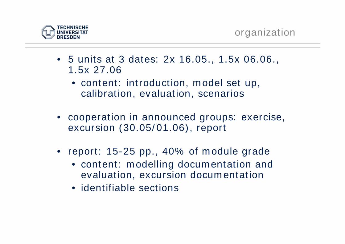
organization

• 5 units at 3 dates: 2x 16.05., 1.5x 06.06., 1.5x 27.06• content: introduction, model set up,

calibration, evaluation, scenarios

• cooperation in announced groups: exercise, excursion (30.05/01.06), report

• report: 15-25 pp., 40% of module grade• content: modelling documentation and

evaluation, excursion documentation • identifiable sections

introduction – what is IWRM

“a process which promotes the coordinated development and management of water, land and related resources, in order to maximize the resultant eco-nomic and social welfare in an equitable manner without compromising the sustainability of vital ecosystems.” 1)

• multipe sectors

• and / or multiple objectives

• and / ormultiple stakeholders

1) Technical Committee of the Global Water Partnership

Schanze & Biegel (2004, modified 2011)Schanze & Biegel (2004, modified 2011)

introduction – why do we model in IWRM

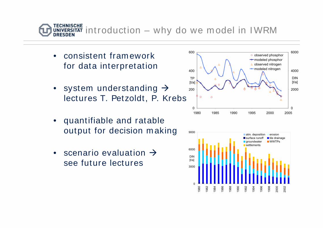
• consistent framework for data interpretation

• system understanding lectures T. Petzoldt, P. Krebs

• quantifiable and ratable output for decision making

• scenario evaluation see future lectures

0

200

400

600

1980 1985 1990 1995 2000 2005

TP[t/a]

0

2000

4000

6000

DIN [t/a]

observed phosphormodeled phosphorobserved nitrogenmodeled nitrogen

0

3000

6000

9000

1980

1982

1984

1986

1988

1990

1992

1994

1996

1998

2000

2002

DIN [t/a]

atm. deposition erosionsurface runoff tile drainagegroundwater WWTPssettlements

introduction- modeling principles

• model (in sciences): abstracted representation of the real world, covering its relevant aspects

• numerical models for matter emission and fluxes:• solution of equations for matter

generation, transport and conversion

• different degrees of spatial distribution, temporal resolution and process description

• purpose-driven selection and application

• integration of different models for sub-systems

Straße 1 Nachklärung

-C-

inflowConstant

yout3

To Workspace4

yN_eff

To Workspace3

yGes_eff

To Workspace2

yVK_eff

To Workspace1yIN

To Workspace

Terminator

Temp

15

T

asm1tmQin

qw Qout

Qw

x

Sctrl

Scope

141000

Sauerstoffzufuhr m³/d

120000

QRSsoll

P

Pump

PC

0

P(tot)

NO NH

WWTP Lviv (VK + Biologie + NK)Version 1.1

Tue Apr 13 10:50:03 2010** Tage Einfahrzeit7 Tage Kalibrierung

start: 30/08/09 00:00:00 = 73415end: 19-Oct-2009 = 734065

Opt. Settings: - rasFlow: 2806

- Vbb: 15600 m³

M

Mixer2M

Mixer1

MechThick1

Manual Switch2

Manual Switch1

Manual Switch

In1Out1Out2

Luftregler

GlobalT

[GlobalT]

2q1minm3d.ma

From File3

m0temp.mat

From File2

m2tn5min.mat

From File1

m2co1min.mat

From File

[GlobalT]

Primary data

ASM1mFracASM1

DO

2804

Constant2

ASM1tmQin qairT

Qe

BB

QRAS

ДобротвірDobrotvir

Кам’Янка Kamyanka

Зах.

Буг

Wes

tern

Bug

Полтва Poltva

Золочівка Zolochivka

ЛьвівLviv

БуськBusk

СасівSasiv

RWQM1

SWAT / SWMM / OGS ASM

SWAT1:200.000

MONERIS

PWF-LU

SWAT1:10.000 rural hot

spot

urban hot spot

CCLMregional climate

temp. resolution 3 h

PWF-LUland use plotwater balance

SWATriver catchment

temporal resolution 1 d

MONERISriver catchment

temporal resolution 1 a

SWMMurban system and water body

temporal resolution: dynamic

OGSsoil and groundwater

temporal resolution: dynamic

RWQM1water body (biology, chemistry)

temporal resolution: dynamic

ASMwaste water treatment plant

temporal resolution: dynamic

CCLM

ДобротвірDobrotvir

Кам’Янка Kamyanka

Зах.

Буг

Wes

tern

Bug

Полтва Poltva

Золочівка Zolochivka

ЛьвівLviv

БуськBusk

СасівSasiv

RWQM1

SWAT / SWMM / OGS ASM

SWAT1:200.000

MONERIS

PWF-LU

SWAT1:10.000 rural hot

spot

urban hot spot

CCLMregional climate

temp. resolution 3 h

PWF-LUland use plotwater balance

SWATriver catchment

temporal resolution 1 d

MONERISriver catchment

temporal resolution 1 a

SWMMurban system and water body

temporal resolution: dynamic

OGSsoil and groundwater

temporal resolution: dynamic

RWQM1water body (biology, chemistry)

temporal resolution: dynamic

ASMwaste water treatment plant

temporal resolution: dynamic

CCLM

WWTP

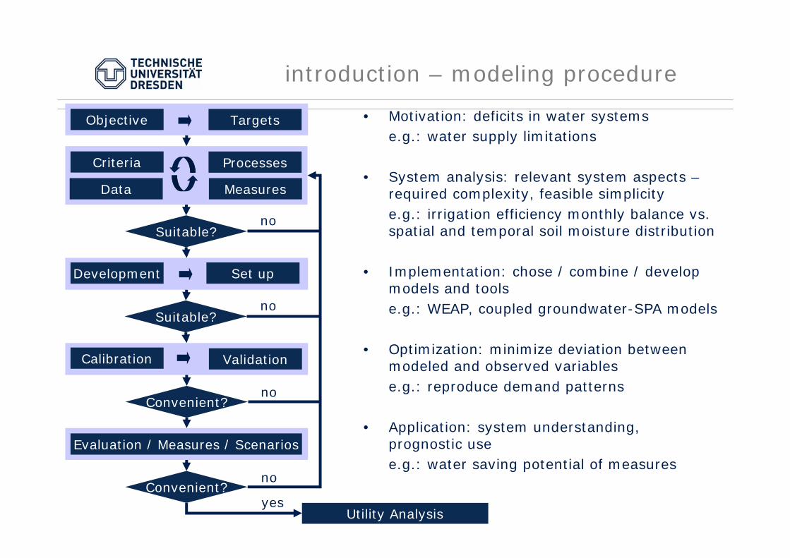
introduction – modeling procedure

• Motivation: deficits in water systemse.g.: water supply limitations

• System analysis: relevant system aspects –required complexity, feasible simplicitye.g.: irrigation efficiency monthly balance vs. spatial and temporal soil moisture distribution

• Implementation: chose / combine / develop models and toolse.g.: WEAP, coupled groundwater-SPA models

• Optimization: minimize deviation between modeled and observed variablese.g.: reproduce demand patterns

• Application: system understanding, prognostic usee.g.: water saving potential of measures

no

Objective Targets

Development Set up

Calibration Validation

Evaluation / Measures / Scenarios

Convenient?

Suitable?

Data

ProcessesCriteria

Measures

Suitable?

Convenient?

Utility Analysis

no

no

no

yes

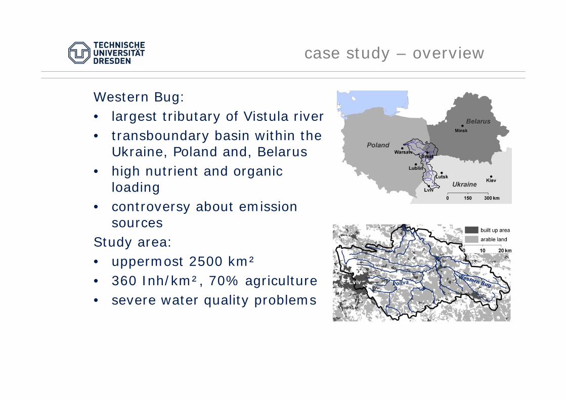
case study – overview

Western Bug:• largest tributary of Vistula river• transboundary basin within the

Ukraine, Poland and, Belarus• high nutrient and organic

loading• controversy about emission

sourcesStudy area:• uppermost 2500 km²• 360 Inh/km², 70% agriculture• severe water quality problems

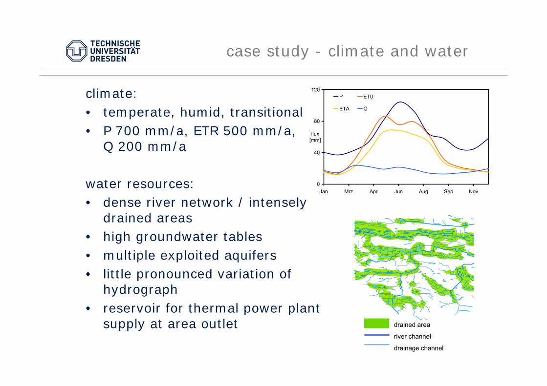
case study - climate and water

0

40

80

120

Jan Mrz Apr Jun Aug Sep Nov

flux [mm]

P ET0

ETA Q

climate:• temperate, humid, transitional• P 700 mm/a, ETR 500 mm/a,

Q 200 mm/a

water resources:• dense river network / intensely

drained areas• high groundwater tables• multiple exploited aquifers• little pronounced variation of

hydrograph• reservoir for thermal power plant

supply at area outlet drained area

river channel

drainage channel

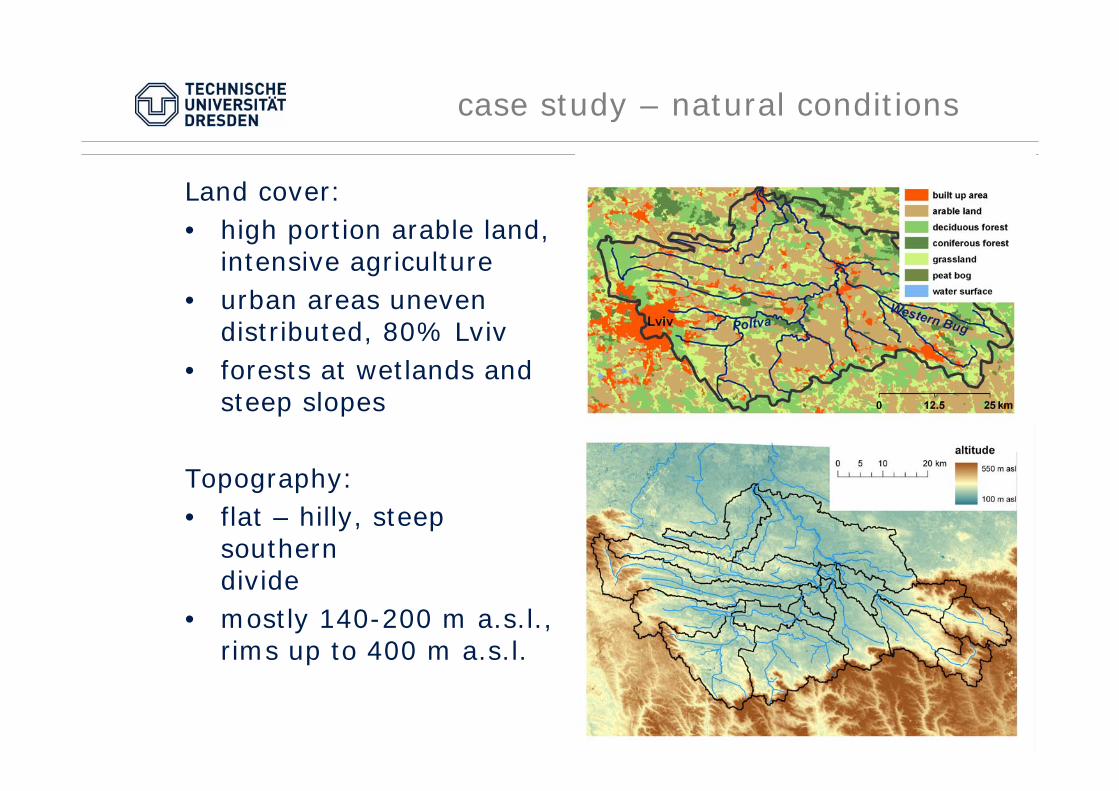
case study – natural conditions

Land cover:• high portion arable land,

intensive agriculture• urban areas uneven

distributed, 80% Lviv• forests at wetlands and

steep slopes

Topography:• flat – hilly, steep

southern divide

• mostly 140-200 m a.s.l., rims up to 400 m a.s.l.

case study - water management

Urban system Lviv:• by far biggest urban structure• weak receiving water: ~2m³/s ww vs.

~1m³/s natural water

Urban systems:• ailing infrastructure, no reinvestments• only settlements >10 000 inh. with

high connection rates

Rural system:• low / no connection to services• water supply and ww disposal to

quaternary aquifer

case study – affected systems

anaerobic river sediment

river water quality deficits

0 50 200 400 600 8000

20

40

60

80

100

min: max: median: mean:

0799105150

NO3 - [mg/L]

Per

cent

ile [%

]

100nitrate in well water

L'viv

Bus'k

Zolochiv

Kamianka Buska

settlement

TN emission [t/a]9 - 100

101 - 200

201 - 500

501 - 1000

1001 - 2000

0 10 205 km

nitrogen emission in subcatchments

case study - stakeholders

• good ecological stateenvironmental NGO

• compliance of limit valuesenvironmental agency

• thermal pollution of river• river water for cooling (qualityand quantity)

thermal power plant

stakeholder requirements pressures

urban population • groundwater for supply• opt. river water for supply

• wastewater to river

rural population • groundwater for supply • wastewater to groundwater

industry • groundwater for supply• opt. river water for supply

• wastewater to river

agriculture • fertilizer excess to groundwaterand river water

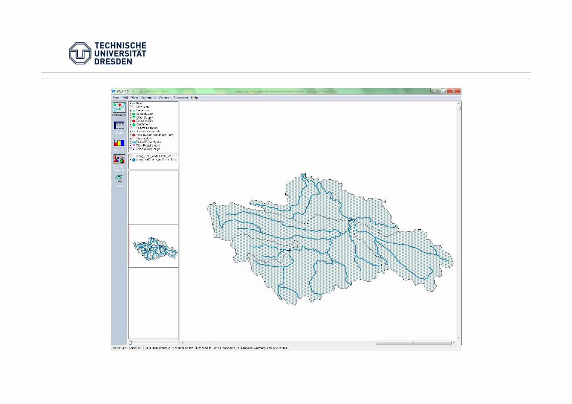
1. SETUP THE SCHEMATIC

Menu

View Bar

Element Window

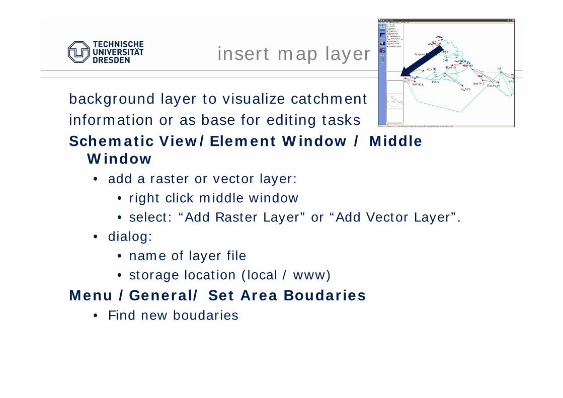
background layer to visualize catchmentinformation or as base for editing tasksSchematic View/Element Window / Middle

Window• add a raster or vector layer:

• right click middle window• select: “Add Raster Layer” or “Add Vector Layer”.

• dialog: • name of layer file • storage location (local / www)

Menu /General/ Set Area Boudaries• Find new boudaries

insert map layer

Save your area

document the progress of model set up and calibration with commented model versions

Menu / Area / Save Version• Select “Save Version”

• comment dialog to describe this version.• Auto-storage of all related sub-files• storage location: WEAP program installation folder.

Menu / Area / Manage Areas• Select “Manage Areas”

• export and import • back up and restore• repair function

Draw a river

Schematic view / Element Window / River• Draw the rivers with higher order first• Click on the “River” symbol in the Element window • Drag the symbol into to the map• Click once for finishing each river segment• Double click to finish drawing the river.

• Name the rivers.

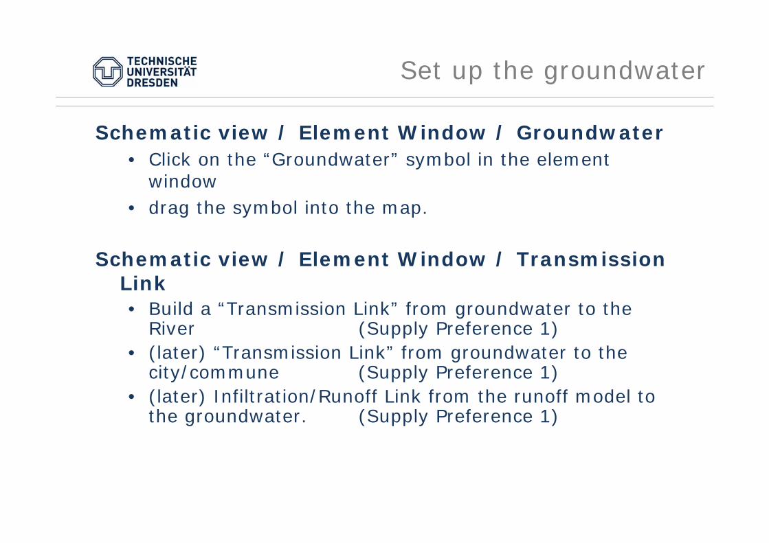
Set up the groundwater

Schematic view / Element Window / Groundwater• Click on the “Groundwater” symbol in the element

window • drag the symbol into the map.

Schematic view / Element Window / Transmission Link• Build a “Transmission Link” from groundwater to the

River (Supply Preference 1)• (later) “Transmission Link” from groundwater to the

city/commune (Supply Preference 1)• (later) Infiltration/Runoff Link from the runoff model to

the groundwater. (Supply Preference 1)

Set up the runoff model

Schematic View/ Element Window/ Catchment• Create a “Catchment” object in the Schematic view to

simulate headflow for the catchment area.• Once positioned, a dialog box will open and request the

following data:

Runoff to Main River Represents Headflow Yes (check box) Infiltration to link the prop. GWIncludes Irrigated Areas No (Default) Demand Priority 1 (default)

Cities and communes

Schematic View/ Element Window/ Demand Site• Pull one demand node symbol for every city and

commune you need into the project area and position it on the map.

Schematic View/ Element Window/ Transmission Link• create a “Transmission Link” from the Groundwater

to the consumers.

Schematic View/ Element Window/ Return Flow• create a “Return Flow” from consumers to the

accordant river/Groundwater

2. SETUP THE DATA

hydrology in WEAP

surface water balance: FAO RR-Methodinput: precipitation P, reference evaporation ET0

direct runoff: R(d) = k(d) * Peffective precipitation: P(eff) = P – R(d)potential evaporation: ETP = k(c) * ET0actual evaporation: ETA = min(ETP, P(eff))runoff: R = P(eff) – ETAinfiltrating runoff: R(inf) = k(inf) * Rsurface runoff: R(s) = R(d) + (1-k(inf)) * R

balance: P = ETA + R(s) + R(inf)

calibration: k(d), k(c), k(inf)

hydrology in WEAP

direct runoff coefficient k(d)• higher in steeper and

more impervious areas

crop coefficient k(c)• plant activity

(transpiration) and increased active surface (leave area)

• scaling parameter for land cover types

infiltration coefficient k(inf)• higher in flatter terrain,

permeable soils

0.0

0.5

1.0

1.5

Jan Mrz Mai Jun Aug Sep Nov

k(c)

urban forestagriculture (corn) wetlandwater

k(d)

A(imp) (Maidment, 2005)

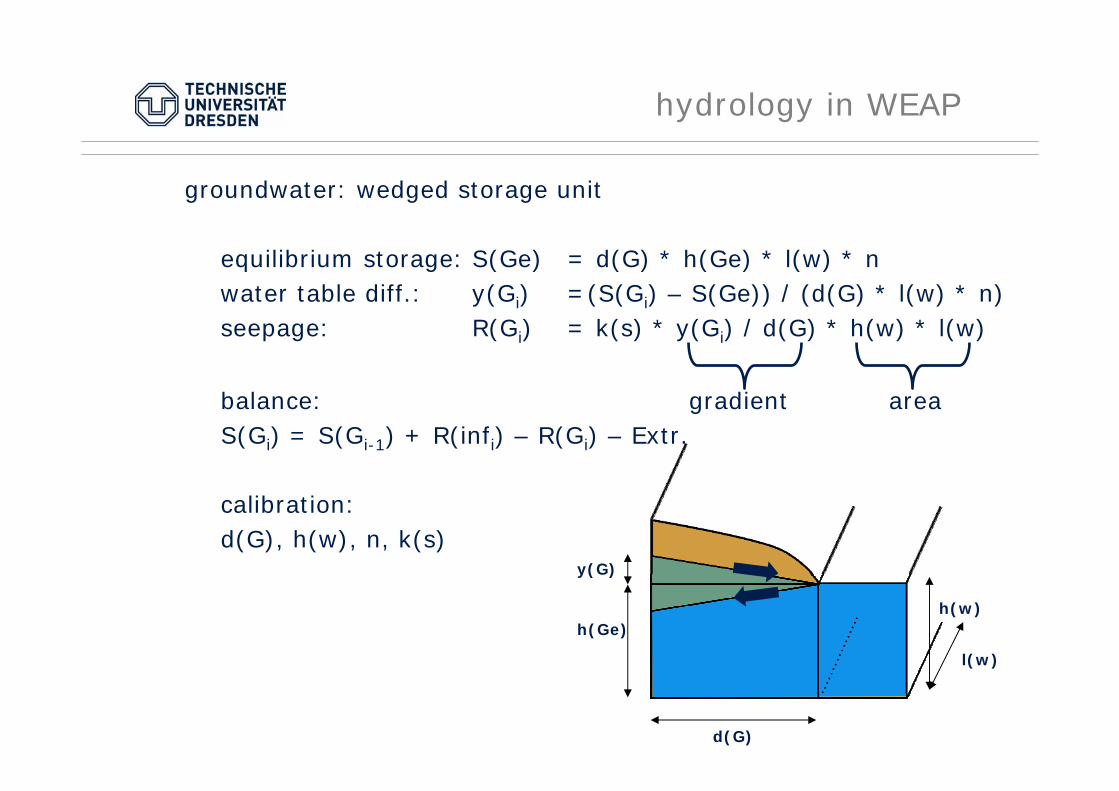
hydrology in WEAP

groundwater: wedged storage unit

equilibrium storage: S(Ge) = d(G) * h(Ge) * l(w) * n water table diff.: y(Gi) =(S(Gi) – S(Ge)) / (d(G) * l(w) * n)seepage: R(Gi) = k(s) * y(Gi) / d(G) * h(w) * l(w)

balance: gradient areaS(Gi) = S(Gi-1) + R(infi) – R(Gi) – Extr.

calibration:d(G), h(w), n, k(s)

d(G)

l(w)

h(w)h(Ge)

y(G)

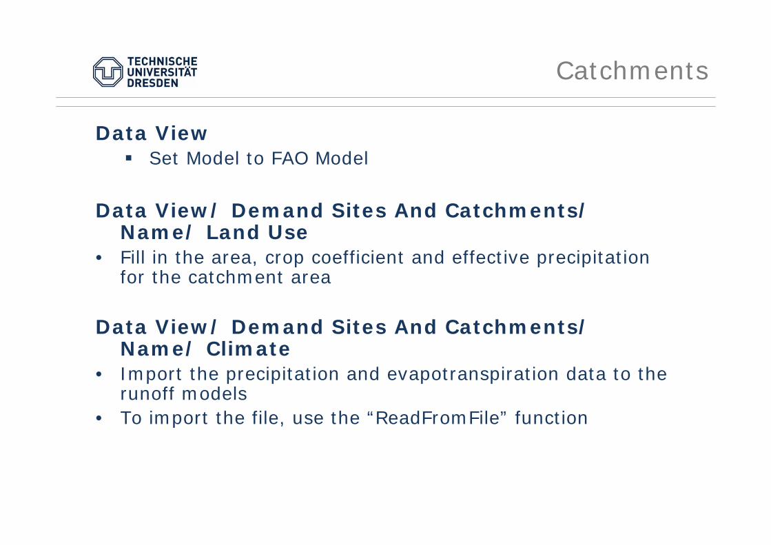
Catchments

Data ViewSet Model to FAO Model

Data View/ Demand Sites And Catchments/ Name/ Land Use

• Fill in the area, crop coefficient and effective precipitation for the catchment area

Data View/ Demand Sites And Catchments/ Name/ Climate

• Import the precipitation and evapotranspiration data to the runoff models

• To import the file, use the “ReadFromFile” function

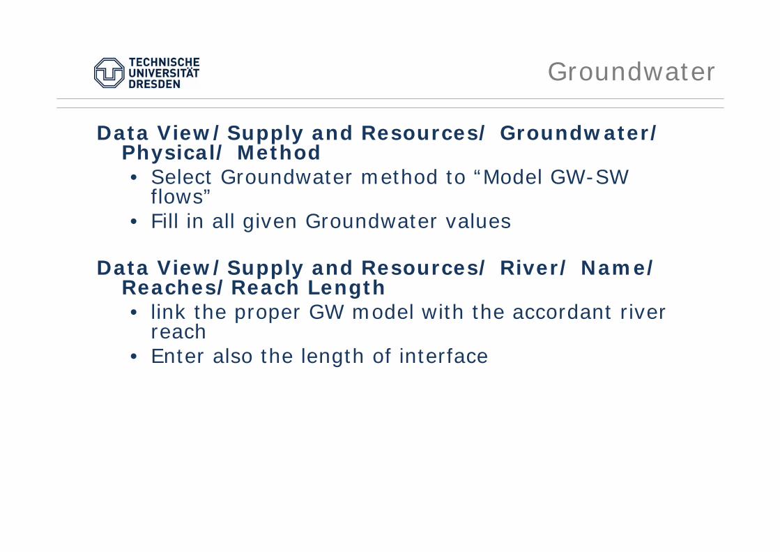
Groundwater

Data View/Supply and Resources/ Groundwater/ Physical/ Method• Select Groundwater method to “Model GW-SW

flows”• Fill in all given Groundwater values

Data View/Supply and Resources/ River/ Name/ Reaches/Reach Length• link the proper GW model with the accordant river

reach• Enter also the length of interface

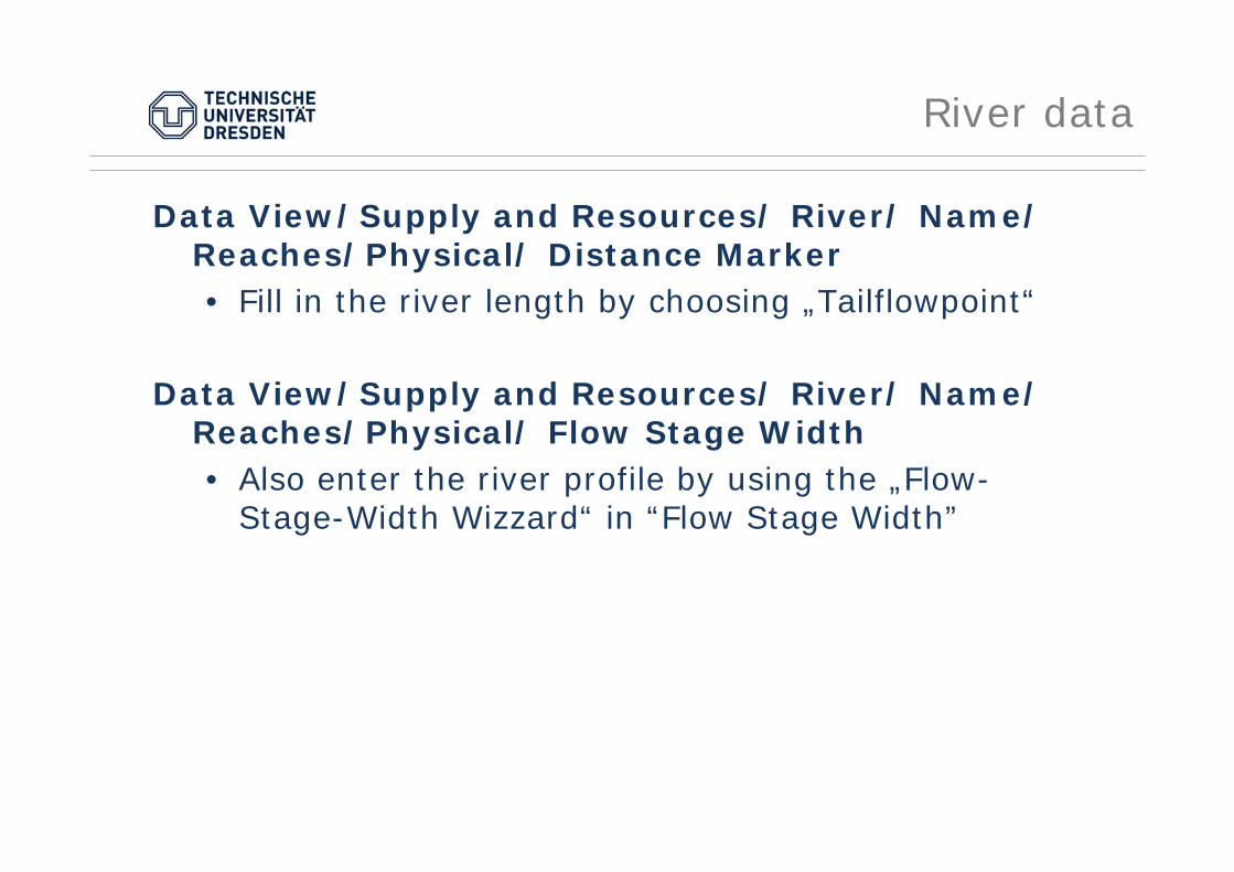
River data

Data View/Supply and Resources/ River/ Name/ Reaches/Physical/ Distance Marker• Fill in the river length by choosing „Tailflowpoint“

Data View/Supply and Resources/ River/ Name/ Reaches/Physical/ Flow Stage Width• Also enter the river profile by using the „Flow-

Stage-Width Wizzard“ in “Flow Stage Width”

Cities and commune

Data View/ Demand Sites And Catchments/ Name/Water Use/ Annual Activity Level• Fill in population

Data View/ Demand Sites And Catchments/ Name/Water Use/ Annual Water Use Rate• Fill in annual water use rate per year of the

according consumers