Article · its complexity is gradually increased to realize a full model that treats non-Fickian...

Subscriber access provided by UNIV OF MARYLAND COLL PARK

The Journal of Physical Chemistry C is published by the American ChemicalSociety. 1155 Sixteenth Street N.W., Washington, DC 20036

Article

Development of a Model for Charge Transport in Conjugated PolymersXuezheng Wang, Benjamin Shapiro, and Elisabeth Smela

J. Phys. Chem. C, 2009, 113 (1), 382-401 • Publication Date (Web): 11 December 2008

Downloaded from http://pubs.acs.org on January 12, 2009

More About This Article

Additional resources and features associated with this article are available within the HTML version:

• Supporting Information• Access to high resolution figures• Links to articles and content related to this article• Copyright permission to reproduce figures and/or text from this article

http://pubs.acs.org/doi/full/10.1021/jp802941m

Development of a Model for Charge Transport in Conjugated Polymers

Xuezheng Wang,† Benjamin Shapiro,‡ and Elisabeth Smela*,†

Department of Mechanical Engineering, UniVersity of Maryland, College Park, Maryland 20742, andDepartment of Aerospace Engineering, UniVersity of Maryland, College Park, Maryland 20742

ReceiVed: April 4, 2008; ReVised Manuscript ReceiVed: October 1, 2008

A finite element model for charge transport in conjugated polymers is developed based on transport equationsfor ionic and electronic charge coupled with the Poisson equation. The model behavior is fully explored, andits complexity is gradually increased to realize a full model that treats non-Fickian diffusion through nonconstantcoefficients and that includes ion transport in the electrolyte. The simulation results are compared qualitativelywith the experimental results for an ion-barrier-covered PPy(DBS) film during electrochemical reduction,and the model is found to successfully account for the dominant behaviors, including the emergence of afront. One of the key findings of the simulations is that migration must be taken into account to correctlydescribe ion ingress: none of the various simulations in which ion transport was only by diffusion predictedthe experimental results. Another is that the front velocity is proportional to the applied voltage, as foundexperimentally, and that the cation front can move into the polymer with a velocity V ∼ �t even when theions move by migration alone.

1. Introduction

Ion and hole transport occur in those applications ofconjugated polymers in which the device operation depends onsignificant changes in the oxidation level of the polymer,including batteries and supercapacitors, electrochromic displays,actuators, and chemical sensors. It is therefore important tounderstand what governs the movements of these chargedparticles in response to an applied voltage in a system in whichtheir local concentrations, as well as the electrical conductivitiesand other properties of the materials through which they move,are changing over time.

The goal of the work in this paper was to develop a generalmodel based on fundamental equations that would account forthe dominant features of charge transport in conjugated polymersduring electrochemical switching between fully oxidized andreduced states. Such a model should ideally have no adjustableparameters and should account for the main effects, if not allthe details. Such modeling based on first principles is not thesame as curve-fitting. The model presented here is also not ablack-box model, such as a lumped parameter equivalent circuitmodel, although such models have been successfully appliedto some aspects of switching behavior (see, for example, refs 1and 2).

The model is focused on ion transport in/out and throughthe polymer since ion ingress is the primary contributor tovolume expansion in actuators and since ion transport is oftenthe rate-limiting step during electrochemical switching. Becauseit is aimed at predicting device performance, the model isphrased on a length scale that is small compared with the devicebut large enough to allow the use of a continuum assumption(see section 3.1.1), which makes modeling by partial differentialequations possible. The model includes ion transport (in thepolymer and also, for the full model, in the electrolyte), holetransport (polarons, bipolarons), and the electric fields that drive

transport (both those that are applied to the material and thosegenerated by the charges themselves). The equations used duringthe initial stages of model development are standard, but theirsimulation is not. Simulation of charge transport in thesematerials has not been done previously, and the details of howthis was done were critical to its success. This paper thus goesinto sufficient detail to enable others to reproduce this work. Inthe later parts of this paper, the transport equations are modifiedto make the coefficients concentration-dependent, and thoseequations are not standard.

The model does not yet explicitly include the effects ofchanges in the packing of the polymer matrix (electrochemicallystimulated conformational relaxation, ESCR, effects) or theelectrochemical reactions themselves (it examines only switchingbetween the fully oxidized and fully reduced states, assumingthat hole transfer between the electrodes is energetically allowedand fast). In other words, the chemical nature of the processand the polymeric nature of the material are ignored in this initialphysical approach, even though under some experimentalconditions the chemical reactions and the conformationalmovements of the chains can be the rate-limiting steps. Includingthese effects in the initial model would be premature and somust be reserved for future work. That is not to say that theseeffects are not critical, but that building a too-complex, all-encompassing model from the beginning does not allow one togain a sufficiently thorough understanding of the reasons forthe model’s behavior to enable confidence in its predictions.ESCR effects are already well-modeled, and joining this newmodel with that one would be a next logical step.

Model development was informed only by the behaviorsobserved during reduction of an ion-barrier-covered film ofPPy(DBS).3,4 If the basic physics of the charge transport isproperly captured by the model, then it should correctly predictwhat happens under other conditions, such as reversing thevoltage to reoxidize the polymer. This will be done in futurepapers.

This modeling work expands upon that done by Lacroix etal.,5 who modeled the movement of electrons and ions in

* Corresponding author. Tel.: 301-405-5265. Fax: 301-314-9477. E-mail:[email protected].

† Department of Mechanical Engineering.‡ Department of Aerospace Engineering.

J. Phys. Chem. C 2009, 113, 382–401382

10.1021/jp802941m CCC: $40.75 2009 American Chemical SocietyPublished on Web 12/11/2008

conjugated polymers, examining several limiting cases analyti-cally. Here, we take the same basic equations governing electronand ion movements, allow their coefficients to be functions ofstate (to, for example, try to capture non-Fickian diffusion),subject them to boundary conditions, and simulate them,allowing us to examine virtually any case of interest. Simulationsoffer the advantage of allowing one to visualize the chargeconcentrations, electric fields, and other variables as they evolveover time. By simulating the geometry described in refs 3 and4, we are able to qualitatively compare the results of thesimulations with the experimental results.

Other prior modeling based on first principles has been donewith the aim of predicting the shape of cyclic voltammograms.Those models used simplifying assumptions to make theproblem tractable, such as that ions moved solely by ordinarydiffusion, that changes in the number of charges on the backbonedid not need to be considered, or that charge neutrality heldeverywhere.6-8 The current model does not make these assump-tions and thus advances that prior work. However, as mentionedabove, in this paper we do not consider the energetics or kineticsof electron transfer between the polymer and the electrode (i.e.,the electrochemistry) and only examine switching to potentialsat which this transfer is possible and fast. Including theinformation on polymer energy levels contained in cyclicvoltammograms is outside the scope of this work but shouldalso be included in future, more sophisticated models.

The main contribution of this paper to our understanding ofoxidation/reduction (redox) in conjugated polymers is a fullycharacterized, physics-based model whose parameters werechosen by taking values from the literature. There was notweaking of parameters to match experimental behavior. Suchfirst-principles modeling is needed to understand device behaviorand to design alternative behaviors. Our simulation code isavailable upon request (a license for the commercial softwarepackage FEMLAB/COMSOL (Comsol AB, www.comsol.com)will be required to run the code).

One of the most important conclusions of this paper is thatno scenario in which the ions move in the polymer solely bydiffusion correctly accounts for the experimental results seenin ref 4; it is necessary to include migration for the model toreproduce the experimental ion profiles. A second conclusionis that this model, despite the fact that it leaves out electro-chemical and polymeric contributions, achieves the goal ofexplaining the dominant behaviors seen during electrochemicalreduction (without adjustable parameters).

The paper is organized as follows. (The reader who is notinterested in modeling details may wish to skip directly to theresults in section 5.) First, a broad overview of the model isgiven in section 2. The modeling methods are detailed in section3: the assumptions, governing equations, boundary conditions,etc. Section 4 explores the behavior of a bare-bones “base case”model. This case is necessary to understand the basic behaviorof the model. Simulations are run to verify that the model givesreasonable results, and the effect of varying the model param-eters is examined. This yields a qualitative understanding ofthe roles of the material constants and boundary conditions. Insection 5, the complexity of the model is increased to betterreflect the physical system, resulting in a “full model”. Modelingcases that address some of the phenomena observed experimental-lyssuch as nonconstant mobilities and non-Fickian diffusionsaswell as cases that address open questions in the literaturessuch aswhether charge neutrality is strictly enforced in the materialsaretreated here. Section 6 summarizes all the model developmentresults, and section 7 ends with a summary and conclusions.

2. Model Overview

In this section, we summarize the effects that are included inthe model and why, based on our understanding of the physicalsystem. The three partial differential equations (PDEs) of themodel are introduced, and terms are defined.

The model presented here explicitly accounts for the move-ment of both ionic charge and electronic charge (polarons andbipolarons on the polymer backbone, referred to herein as“holes” in analogy to the positive charges in inorganic semi-conductors). In prior versions of this model, hole transport waseither neglected9 or the assumption was made, based onexperimental estimates in the literature of the relative mobilitiesof the polarons and the ions, that the holes move instantaneouslyrelative to the ions.10 The latter approach allowed us to formulatean analytical solution for the hole transport. This simplifyingassumption has been lifted here.

There are three mechanisms for charge transport: diffusion,drift (also called migration), and convection. Diffusion occursin the presence of concentration gradients. Fickian diffusionarises when the probabilities for particle movement are equalin all directions, i.e., if the medium is isotropic. (However, sincethe properties of these polymers are not isotropic during redox(see ref 4, Figure 2), diffusion cannot be Fickian.) Migration isthe movement of a particle under a force, such as the movementof a charged particle under an applied voltage. As reviewed byLacroix,5 the existence of electric fields in the polymer,particularly in the reduced regions, must be taken into account.Since both ions and holes are charged species, one cannot apriori neglect their movement in electrical fields nor theirelectrostatic interactions. Electrochemists have traditionallycombined drift and diffusion in the electrochemical potential.11

For transparency, they are kept separate here. Lastly, convectionis the movement of a particle carried in the flow of a fluid, likea boat in a current. This last mechanism is neglected in ourmodel. For ion transport, it is neglected because there are nosignificant fluid flows through the conjugated polymer (althoughsolvent diffuses into the polymer independently of ion trans-port,12 this occurs at a slower time scale and does not carryions). For hole transport, it is neglected because the polymerchains do not flow as a liquid does (although the chains doundergo local movements such as changes in conformation).In the electrolyte, convection is also neglected since the solutionis unstirred. Thus, the model includes one partial differentialequation (PDE) for the ion current due to drift and diffusionand a second PDE for hole drift and diffusion.

The electric fields under which the charges move arise fromtwo sources. Physically, fields are produced by applied voltageson the electrodes and by local imbalances between the concen-trations of positively and negatively charged species. It onlytakes a tiny charge imbalance to create a large electric field,which means that even if charge neutrality is satisfied almosteverywhere net charge can still become the dominant driverfor ion transport.5 In the model, boundary conditions are usedto specify the potentials at key interfaces, and Poisson’sequation, a third PDE, relates the gradient of the electrical fieldinside the polymer to the net charge.

The three PDEs are coupled because the concentrations ofholes and ions in the polymer depend on each other (net chargeresults in electric fields, which leads to charge migration). In acation-transporting polymer like PPy(DBS), as holes are with-drawn at the electrode, charge compensating cations enter fromthe electrolyte. The negatively charged DBS- counterions(anions A) are immobile in the polymer and are treated as afixed background in the model. The concentrations of holes H

Model for Charge Transport in Conjugated Polymers J. Phys. Chem. C, Vol. 113, No. 1, 2009 383

and cations C sum to the concentration of anions almosteverywhere, and where they do not, charge neutrality is violatedand electrical fields are produced that result in charge migration.

The equations used in our work are similar to the standardones for describing charge transport in crystalline inorganicsemiconductors like silicon13 and therefore may be too simpleto account for all the physics occurring in the conjugatedpolymer during redox, a process that has no inorganic analog.However, they provide a first approximation, a starting pointin the model-building process. We show in this paper that theydo, in fact, account for much of the behavior seen experimentally.

Since the equations are coupled and since they have nonlinearparameter dependencies, they cannot be solved analytically forany general case. Thus, they are solved numerically using finiteelement modeling. After solving for the initial conditions (thepolymer is either fully oxidized or fully reduced before aswitching potential is applied at the boundaries), the ion, hole,and potential profiles are allowed to evolve in response to eachother, simulating the redox process.

Model development was informed only by experimentalresults obtained during electrochemical reduction of an ion-barrier covered film of PPy(DBS). Comparison between simula-tion and experimental results guided the choice of initial andboundary conditions, meshing and other details of the simulationmechanics, and choices such as how to stipulate the maximumconcentration of ions in the material. In later papers, we shallrun the model “backwards” by reversing the voltages at theboundaries to simulate oxidation and shall modify the third PDEto reflect anion transport to simulate redox in materials such asPPy(ClO4).

3. Modeling Methods

This section contains the information required to reproducethe work in the remainder of this paper, as well as in subsequentpapers that will utilize this model. Readers who are not interestedin the internal workings of the model should skip to section5.2.2. The assumptions going into the model and a justificationof the continuum treatment are given. We describe how themodel is derived and discuss the physics that were included.The governing equations are presented, as are the boundaryconditions. Methods for reducing model complexity are de-scribed, as is the way the nondimensionalization was performed.Finally, the numerical methods are described, i.e., how theresulting equations were actually solved numerically.

3.1. Model Properties. 3.1.1. Continuum Treatment. Thefinite element model volume elements are 10 nm on each side.This is small compared to device length scales but largecompared to polaron length scales, so it is appropriate to use acontinuum assumption. Within each volume element, there aremany ions and/or holes (there are ∼103 holes in a volumeelement), so that it is appropriate to consider concentrations ofspecies instead of tracking individual molecules. (This estimatecame from the following. To deposit a film 1 µm thick consumes200 mC/cm2,14 approximately 10% of which is used for thecreation of charge carriers: [0.1 × 200 × 10-3 C/(cm2 ·mm)/(106 × 106 × 102)]/1.6 × 10-19 C/electron ≈ 1000 electrons/(10 nm)3.)

3.1.2. Physics and Equations. 3.1.2.1. GoVerning Equations.The first modeling equation (the continuity equation15) expressesthe conservation of species

∂Ci

∂t)- ∇ · Jbi (1)

where Ci is the concentration of species i (mol/cm3) and Ji isthe flux (mol/s cm2). Ci is a dynamic variable that depends on

space and time, so Ci ) Ci(x,y,z,t). This equation has no source/sink terms and thus holds in the absence of species generation(e.g., by light) or annihilation.

The flux Ji must be expressed in terms of the physicalconditions. As mentioned previously, we ignore convection butconsider diffusion and drift, Jb) Jbi

diff + Jbidrift. Commonly used

models for each of these components in inorganic semiconduc-tors are11,13

Jbidiff )-Di ∇ Ci (2)

where Di is the diffusion coefficient (cm2/s) and

Jbidiff ) ziµiCiEb (3)

where zi is the positive or negative charge per species molecule;µi is the mobility (cm2/V s); and Eb is the electric field, andwhere Eb ) -∇ O and O is the electric potential. (There are ofcourse other ways of formulating the currents, involving, e.g.,quasichemical potentials,16 particle jump probabilities in differentdirections,17 etc.; we began with the simplest.) The assumptionscontained in these two equations are described in refs 13 and18. The expression for the diffusion flux, for example, assumesthat the particles take a random walk that is unaffected by otherparticles (dilute solution approximation), and it does not applyin systems in which the particles hop between a fixed numberof sites.

Substituting the flux equations into eq 1 results in a PDE forthe rate of change of the concentration of species i (the cationsor the holes) at any location inside the polymer

∂Ci

∂t)- ∇ · Jbi )- ∇ · (-Di ∇ Ci - ziµiCi ∇ O) (4)

In this framework, Di and µi are not constants but are functionsof the oxidation level of the polymer. (It is possible that theyare also functions of other variables, and part of the job of futuremodeling will be to determine the complete functional depen-dence of these coefficients.)

In systems at equilibrium with noninteracting particles thatundergo random walks and that have a density given by theBoltzmann distribution, Di and µi are related through the Einsteinrelation: Di/µi ) kT/q ) RT/F.13,16,17 In these systems, eq 4 isequivalent to the Nernst-Planck equation.11 The advantage ofthe Einstein relation is that it reduces the number of independentcoefficients that must be determined. Unfortunately, sincediffusion during redox is not Fickian and since the density ofthe ions (or holes) is so high in the fully reduced (oxidized)states that they cannot realistically be considered to be nonin-teracting, this assumption cannot be made, and the model mustexamine the effect of a varying D/µ (see section 4.3.2). Forexample, in systems with memory, in which the direction of aprevious step affects the direction of the next step, the ratioD/µ is concentration dependent.17 A more general relation-ship is

Di

µi)

Ci

q∂Ci

∂η

(5)

where η is the chemical potential. It has been shown that usingthis relationship with a Gaussian density of states accounts wellfor the increase in D/µ with concentration seen in disorderedorganic semiconductors.19

Maxwell’s electrostatic equation (Poisson’s equation) is usedto model the electric fields, giving the potential in terms of thenet charge density Q (C/cm3).

384 J. Phys. Chem. C, Vol. 113, No. 1, 2009 Wang et al.

ε0∇ · (ε∇ O))Q)∑i)1

n

ziCi (6)

Here εo is the permittivity of a vacuum; ε is the dielectricconstant of the material; and zi is the (positive or negative)charge of the ion or hole. In this paper, we used zi ) 1 for boththe holes and the ions and did not consider, e.g., divalent cations.

Equations 4 and 6 encompass the Nernst equation, which isderived by balancing the drift and diffusion terms at equilibrium.In fact, the formulation here is more general since the systemis not at equilibrium during oxidation/reduction.

In this model, ion transport is not coupled to mechanical stressusing a PDE (in the real system, ion ingress is responsible forvolume change, and thus actuation stress in the polymer). Rather,this coupling is handled (section 5.1) artificially using anempirical form for the dependence of the diffusion coefficienton ion concentration, obtained in ref 4 (Figure 15). Couplingmechanical effects into the model, such as due to polymerstiffness, conformational changes, or actuation strain, shouldbe the subject of future work.

3.1.2.2. Boundary and Initial Conditions. In the previoussection, the treatment of the movement of charged species withinthe polymer was explained. To solve the PDEs of eqs 4 and 6,it is necessary to define boundary conditions (i.e., voltages,fluxes) and initial conditions. The boundary conditions (BCs)describe how the charges get in and out of the material, andthey should correspond to the physical conditions imposed atthe polymer/electrode and polymer/electrolyte interfaces. They

must not only be chosen to make physical sense and lead tophysically meaningful results but also they must allow thesimulations to run.

At the polymer/electrode boundary, there is no ion flux acrossthe interface, as shown in Figure 1 (JbC · n ) 0, where n is a unitvector oriented perpendicular to the boundary). For the holes,a flux boundary condition was used at the electrode. Duringreduction, we set

JbH )µHHEb (7)

With this expression, the higher the electric field Eb and thehigher the hole concentration H in the polymer, the higher thecurrent density crossing from the polymer to the electrode. Whenthe hole concentration falls to 0, current flow between thepolymer and the electrode ceases. Since the simulation cannotsolve for H if H is also used in the boundary condition, in themodel this is actually phrased as JbH ) µH(1 - C)Eb, which istrue almost everywhere by charge neutrality. This flux boundarycondition was used in the 1D model. It could not, however, beused in the 2D simulations since it caused them to “crash”.Instead, the 2D model used a constant hole concentration C0 atthe polymer/electrode boundary. To confirm that this gave thesame results, the 1D model was run with the concentration BCand compared to the 1D model with the flux BC, and the resultswere the same. Furthermore, the results of the 1D and 2Dsimulations with C0 at the polymer/electrode interface werecompared, and these results were also identical.

During oxidation, this boundary condition was changed to

JbH )µHCEb (8)

because the current now depends on the number of availablesites onto which a hole can potentially be placed, which is equalto the number of sites occupied by cations. The question arisesas to whether to use the ion or hole mobility in these expressionssince ion transport is the rate-limiting step. It turns out that usingeither µH or µC gives identical results.

The potential V at the electrode boundary in the model is,approximately, the applied oVerpotential in the experiments, i.e.,the difference between the applied potential and the potentialat which reduction (or oxidation) begins. This is distinct fromthe experimental applied potential (vs Ag/AgCl) because onlyfully oxidizing or reducing potentials can be applied in the modelsince the model does not yet take into account the energeticsof charge transfer seen in the cyclic voltammogram. Theelectrode/polymer boundary condition used in the model isequivalent to stipulating that there is sufficient energy to allowthe holes to cross the interface, in either direction, in responseto the electric fields. Note also that in the model, setting O )-1 V at the electrode and O ) 0 V at the electrolyte interfaceis equivalent to setting O ) 0 V at the electrode and O ) +1 Vat the electrolyte, since only the potential difference is significantin the mathematics.

At the polymer/electrolyte boundaries, there is no hole flux(JbH · n ) 0) since holes cannot enter the electrolyte. In the initialmodeling cases (section 4), which do not include transport inthe electrolyte, a constant ion concentration (C ) Cmax) isimposed at the boundary during reduction, where Cmax is themaximum concentration of ions in the polymer. (The effect ofvarying this boundary condition is shown in the SupportingInformation, section 2.6.) Also in the initial cases, the potentialat this interface is set to zero (O ) 0). This is not physicallyreasonable, since it ignores the resistive drop in the electrolyte,and thus causes the model to neglect the effects of changing

Figure 1. (a) Schematic of the physical system, showing the potentialson the working (WE) and reference/counter (RE) electrodes duringelectrochemical reduction of a cation-transporting polymer covered byan ion barrier, the bulk concentration of cations in the electrolyte(0.03Cmax), and the interfaces that ions (C) and holes (H) can cross.(b) The PDEs used in modeling this cation-transporting conjugatedpolymer. (c) The boundary conditions used at the polymer interfacesfor a basic model that does not include ion transport in the electrolyte(the “base case” model of section 4).


electrical conductivity during redox. Therefore, in section 5.2we expand the model to include the electrolyte.

The top polymer/insulator boundary has no ion or hole flux(JbC · n ) 0 and JbH · n ) 0), and it is electrically insulating (∇ O · n) 0). This boundary does not appear in the 1D simulations.

The initial conditions were an ion concentration of 0 and ahole concentration of H ) Hmax everywhere, representing thefully oxidized state. The initial potential profile was found bysolving the electrostatic PDE (eq 6) based on initial ion andhole concentrations.

3.1.3. Reducing Model Complexity. Two strategies were usedto reduce the model complexity: (a) nondimensionalizing themodel to reduce the number of free parameters and (b) reducingthe number of spatial dimensions by exploiting symmetry orphysics. Reducing complexity is important for running themodels in a reasonable period of time, for reducing the numberof independent parameters, and for running the models stably(i.e., without crashing). This leads to the introduction of the1-D model that was used to generate most of the results in thepaper and a description of how this relates to the physicalsystem. Finally, we describe the transformation of the numericalvalues of the physical system described in ref 4 to thenondimensional values used throughout the simulations.

3.1.3.1. Nondimensionalization. Nondimensionalizing (i.e.,normalizing) the model reduces the number of parameters tothose that are actually independent. The nondimensional pa-rameters better illustrate the balance between competing physicaleffects since each nondimensional parameter represents a ratioof dimensional parameters, and they allow a single modelingrun to predict the behavior of a whole range of dimensionalparameters. An excellent discussion of the benefits of nondi-mensionalization is provided in ref 20.

Essentially, each dimensional variable is normalized by acharacteristic scale of the system (see Table 1). For example,

the nondimensional length x was obtained by taking thedimensional length x (µm) and dividing it by the maximum ionpath length L ) 150 µm, a length that characterizes the size ofthe experimental system, so x ) x/L. The boldface variablesdenote dimensional quantities, and the plain text variables denotenondimensional variables. Ion and hole concentrations werenondimensionalized by Cmax ) Hmax ) 3 M, the estimatedmaximum concentration of ions/holes in the polymer. Allnondimensional variables are unitless. The nondimensionaliza-tion of the remaining variable and the resulting PDEs are derivedin the Supporting Information (SI section 1.1).

The nondimensional governing equations for cation and holetransport are

(a)∂C∂t

)- ∇ · (-DC ∇ C-C ∇ φ)

(b)∂H∂t

)- ∇ · (-DH ∇ H- µHH ∇ φ)

(c) ∇ (ε ∇ φ))Q)C+H- 1 (9)

where µC is not shown in the first equation because it is equalto 1. The dimensional model, eqs 4 and 6, has eight freeparameters: DC, µC, DH, µH, ε, V, L, and H0. The nondimen-sional model, eq 9, has four: DC, DH, µH, and ε.

3.1.3.2. Reduced Spatial Dimensions. PDEs are solved infinite element models by meshing the computational region inspace into cells (nodes) and then iterating all the variables (ionand hole concentrations and electric potential) in time acrossall the spatial nodes. Increasing the number of spatial dimensionsincreases the computational cost, by the square in going from1-D to 2-D and by the cube in going to 3-D. Therefore, westarted with fast-running 1-D models for initial model develop-ment (less than 1 min of run time) and proceeded to 2-D models(20 to 30 min of run time) once we were satisfied with thequalitative predictions. By the symmetry of the experimentalgeometry, which had no variation along the long axis of thepolymer stripe, 3-D models were not required.

The 1-D models were numerically more robust than the 2-Dmodels because they had fewer nodes and required less computermemory. The 2-D models, operating near the limit of computermemory and speed, were more fragile, “crashing” in severalcases, such as when large gradients were created that were notwell resolved by the mesh. In addition, when numerical issuesarose, such as resolving steep gradients, including sharp cutofffunctions to prevent the charge from going above Cmax or Hmax

(charge capping), or capturing small dielectric coefficients, the1-D models could be solved by increasing the mesh resolution.

At t ) 0, the electric field lines form arcs through the polymerbetween the electrode and the electrolyte. Conceptually, the 1-D

Figure 2. (a) A schematic 2-D slice across an ion-barrier-covered,oxidized PPy(DBS) strip at t ) 0, showing calculated electric fieldlines (white) going from the electrode to the electrolyte prior to anyion ingress. The 1-D model can be considered to represent ions andholes traveling along one of these field lines (such as indicted by theblack line). For clarity, the vertical axis is much exaggerated incomparison with the experimental geometry. (b) The geometry studiedin the 1-D models is equivalent to a line between the electrolyte andthe electrode.

TABLE 1: Nondimensional Units and Variables

unitless variabledefinition (from

dimensional variables) description characteristic quantity used for normalization

x, y, z x/L, y/L, z/L distance L ) maximum ion path length∇ L∇ gradientφ O/V0 applied overvoltage on electrode V0 ) 1 VC, H C/Hmax, H/Hmax ion, hole concentrations

in the polymerHmax ) maximum concentration in the polymer )

number of immobile dopant anionst t/[L2/µCV] time t0 ) L2/µCV ) characteristic time ) characteristic

length /ion drift speed∂/∂t [L2/µCV]∂/∂t time derivative from definition of t, by chain ruleµC 1 cation mobility becomes unity through choice of t0

µH µH/µC hole mobility µC ) cation mobilityDC DC/µCV cation diffusivity cation driftε εV/L0

2Hmax dielectric constant characteristic voltage gradient andcharge concentration (using zi ) 1)


simulation can be considered to be along one of these lines, asshown in Figure 2. Note that this is the case because nonucleation occurs in PPy(DBS). To simulate nucleation inpolymers such as PPy(ClO4), in which ion ingress begins alongvertical lines,21 a 2-D or 3-D model would be needed.

Figure 2b is the same geometry as for a layer of conjugatedpolymer on an electrode uncovered by an ion barrier, so themodel should correctly predict the behavior for this case as well.The question arises, how much does the transport differ in theion-barrier covered case, due to the distortion of the field lines,from the thin film case? This question is taken up in section4.2, in which the 1-D simulation is compared to a 2-Dsimulation.

3.1.3.3. Parameters. Of the eight dimensional model param-eters (DC, µC, DH, µH, ε, V, L, and H0), three are known: V is1 V, L is 150 µm, and H0 is 3 M. The static dielectric constantε depends on the doping level, varying between 4 in the undopedstate (close to typical values for polymers) to 1000 in the fullydoped state for polyaniline;23 values are similar for doped PPy.22

(The dielectric constant also depends strongly on temperatureand frequency.22) DC and µC only come into the model as aratio, and initially a ratio of 0.026 was used, taken from theEinstein relation D/µ ) kT/q ) 0.026 V.13 The coefficients forthe holes were defined relative to those for the ions, and in thebaseline model case (section 4.1), they were taken to be 1000times larger, so DH ) 26 and µH ) 1000. The choice of thefactor of 1000 was somewhat arbitrary: it is known that holetransport is much faster than ion transport but not by how much.The choice of 1000 was enough to make hole transport virtuallyinfinitely fast relative to ion transport for the configuration usedin ref 4.

3.2. Numerical Methods. This section discusses the methodsused to solve the equations, as well as the computational issuesthat were encountered (meshing, stability) and how they wereovercome. For example, the ways we handled the inability touse a physically reasonable value for the dielectric constant isdescribed.

3.2.1. General. The nondimensional PDEs were solved usingthe PDE modeling software FEMLAB (COMSOL), version 3.2.Of the three PDEs in eq 9, the first two are dynamic (theycontain time derivatives d/dt), and the last one is static. Weproceeded by choosing initial conditions for C and H at t ) 0and solving the electrostatic PDE for the potential φ that satisfiedthe boundary conditions. Using starting variables C(x,y,t ) 0),H(x,y,t ) 0), and φ(x,y,t ) 0), FEMLAB then solved the PDEsat each time step and updated the variable values to find C, H,and φ at t ) ∆t, 2∆t, 3∆t, ..., T, where T is the simulation endtime.

We used a number of techniques to enable and improve thenumerical simulations since numerical solution schemes for drift/diffusion PDEs can suffer from numerical instability andspurious oscillations, particularly in simulations with sharppropagating fronts. As is standard in numerical methods, a smallamount of artificial diffusion was added to stabilize thesimulations (this does not change the character of the solutions).Specifically, we added the Petrov-Galerkin compensatedartificial diffusion available within FEMLAB24 to both hole andion transport (using a tuning parameter of 0.25). For consistency,we used this in all the simulations, even in cases that alreadyhad a significant amount of diffusion.

The smaller the dielectric constant ε, the smaller the regionsin which charge neutrality is violated. For the experimentallyreasonable values of ε given above, the nondimensionaldielectric constant ε is on the order of 10-11, yielding regions

that are so thin that the mesh density required to resolve themwas beyond our computing capabilities, even for the 1-D model.Therefore, the models were run with the smallest dielectricconstant that could be resolved, ε ) 10-3. We then verifiedthat as ε decreased the behavior of the model converged(Supporting Information section 2.1, or SI 2.1). We also rancases with charge neutrality strictly enforced (ε ) 0). (In theSupporting Information, we show how the charge-neutralequations can be derived from the governing equations 9a-c,and we show that the charge-neutral behavior is exactly the limitof the small-ε behavior as ε f 0.)

3.2.2. 2-D Simulations. For the 2-D simulations, there wereadditional computational issues. First, finer meshing was neededin regions where the electric field changed rapidly. This wasdone, after solving for the initial potential, by allowingFEMLAB to adapt the mesh spacing given that potential profileand using the same mesh in all subsequent simulation steps.(This mesh is thus optimized for the potential profile at t ) 0and not for later times. This means that the mesh will not beoptimized during the entire simulation since FEMLAB cannotperform real-time adaptive meshing.)

Second, the 2-D the geometry posed some additional chal-lenges. In the experiments, the thickness of the polymer (300nm) was small compared to its half-width (150 µm), giving anaspect ratio (height:width) of 1:500. This configuration couldnot be used directly because it was numerically unstable: if thethickness (z-direction) was discretized into 10 nodes and thewidth (y-direction) into 100 nodes, then each grid element hadan aspect ratio of 1:50 () 0.03/1.5). However, numerical errorsincrease as mesh elements deviate away from an aspect ratioof 1. To address this problem, the simulated film thickness wasinstead set to be 100 times thicker than the actual film thicknessand both directions discretized into 100 nodes, so that the gridelements had an aspect ratio of 1:5. To correct for the increasedthickness, D, µ, and ε in the y-direction (thickness direction)were increased, creating anisotropic diffusion, migration, anddielectric coefficients and making the film act as if it werethinner. To compensate for the 100-fold increase in thickness,these parameters should have been increased by a factor of 1002,with the square arising from the spatial second derivatives ineq 9. However, the largest anisotropy for D and µ that was stablein the simulations was 1000. Thus, the simulation geometry wasequivalent to a film with an aspect ratio of 1:158. The dielectricconstant was only increased by a factor of 10 (giving at leastsome degree of anisotropy) since it was already too large, andincreasing by 10 000, it would have moved ε even further awayfrom realistic values.

With boundary conditions as shown in Figure 1c, the sharpsquare corners, where the electric fields become highly con-centrated, led to numerical instabilities. The electrode/electrolyteand ion-barrier/electrolyte corners were therefore beveled to a45° angle. Also, with two different potentials applied at thepolymer/electrode and polymer/electrolyte interfaces, there wasa voltage step at the vertices (see Figure 1c). Experimentally,this does not arise because the electrolyte is not a perfectconductor, and the voltage at the corners will blend smoothlyfrom φ ) -V (polymer/electrode) to φ ) 0 (polymer/electrolyte). An exponential decay was used in the simulationsto smoothly change the voltage from the electrode/electrolytecorner to the electrode edge.

4. Results 1: Base Case Model and Variations

In this section, we present the results of running a simplestcase model so that its basic behavior can be understood, i.e.,


not only what the model predicts but also why, beforecomplexities like an electrolyte layer are added. As we showbelow, this model is sufficient to describe most of the resultsseen experimentally during the reduction of a PPy(DBS) stripecovered with an ion barrier. The benefits of running simplemodels include transparency in understanding the outcomes aswell as faster and more robust simulations. However, as weshall show in later papers, other experimental geometries requiremore sophisticated models.

As discussed above, the model was built based on electro-chemical reduction of a cation-transporting material. To beginthe modeling effort, we started with a base case, which was thesimplest case, and then increased the model complexity stepby step, proceeding to the more difficult, and realistic, cases.This section is thus presented as a theme (the base case) withvariations, the latter being used both to confirm that the modelwas behaving reasonably, i.e., predicting behavior that wasqualitatively consistent with the experiments, and to give a firmunderstanding of how the model behaved and why. Results areprimarily from the 1-D model, with 2-D simulations run whennecessary for confirmation. After this, the model complexitywas increased by adding nonconstant coefficients as well astransport in the electrolyte.

Since the base case is the simplest, it only includes transportin the polymer (not in the electrolyte yet). As mentioned above,the material coefficients DC, DH, µC, µH, and ε depend on thestate of the polymer; they can be functions of ion concentrationC, hole concentration H, and the electric potential φ. However,in the base case, these coefficients were all treated as constant.

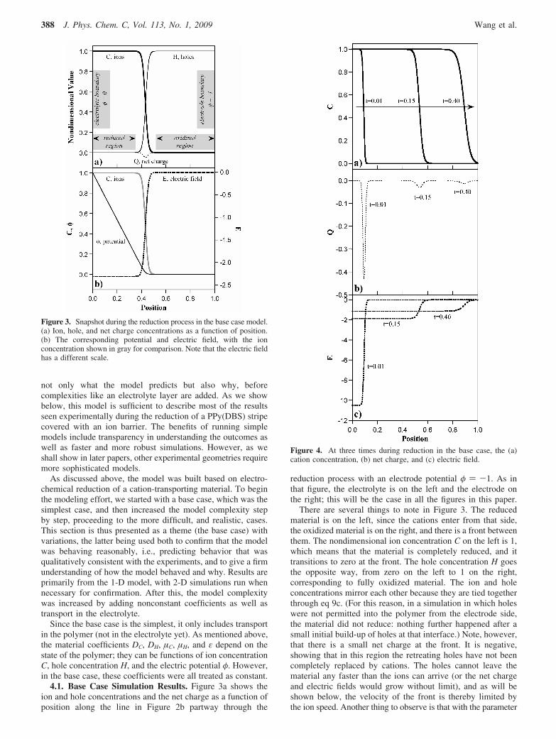
4.1. Base Case Simulation Results. Figure 3a shows theion and hole concentrations and the net charge as a function ofposition along the line in Figure 2b partway through the

reduction process with an electrode potential φ ) -1. As inthat figure, the electrolyte is on the left and the electrode onthe right; this will be the case in all the figures in this paper.

There are several things to note in Figure 3. The reducedmaterial is on the left, since the cations enter from that side,the oxidized material is on the right, and there is a front betweenthem. The nondimensional ion concentration C on the left is 1,which means that the material is completely reduced, and ittransitions to zero at the front. The hole concentration H goesthe opposite way, from zero on the left to 1 on the right,corresponding to fully oxidized material. The ion and holeconcentrations mirror each other because they are tied togetherthrough eq 9c. (For this reason, in a simulation in which holeswere not permitted into the polymer from the electrode side,the material did not reduce: nothing further happened after asmall initial build-up of holes at that interface.) Note, however,that there is a small net charge at the front. It is negative,showing that in this region the retreating holes have not beencompletely replaced by cations. The holes cannot leave thematerial any faster than the ions can arrive (or the net chargeand electric fields would grow without limit), and as will beshown below, the velocity of the front is thereby limited bythe ion speed. Another thing to observe is that with the parameter

Figure 3. Snapshot during the reduction process in the base case model.(a) Ion, hole, and net charge concentrations as a function of position.(b) The corresponding potential and electric field, with the ionconcentration shown in gray for comparison. Note that the electric fieldhas a different scale.

Figure 4. At three times during reduction in the base case, the (a)cation concentration, (b) net charge, and (c) electric field.


settings of the base case the migration component of the fluxmakes a substantial contribution to the transport, as evidencedby the existence of a front. (Since we are using constantcoefficients with a Fickian diffusion equation, the front cannotarise from the diffusion component.)

To relate these curves to the experimental work, the ionconcentration should be compared with Figures 5 and 7 in ref4 (see also ref 9). The ion concentration in Figure 3a, whenmirrored around the y-axis, corresponds to intensity in theexperimental profiles. There is good qualitative agreement.

Figure 3b shows the electric field and the potential at thesame instant of time. There is almost no potential drop acrossthe oxidized region of the film; instead, the voltage is droppedacross the reduced region. This is the result one would expectfrom a consideration of nondimensional material conductivity,given by

σ(x))C(x)µC +H(x)µH ∼ H(x)µH (10)

since µH/µC ) 1000. In the model, this outcome arisesautomatically from the transport equations. The cation and holefluxes due to migration are expressed as JC

drift ) zCµCCCE )σCE and JH

drift ) zHµHCHE ) σHE (where zC ) zH ) 1).Therefore, the migration current density is

Jdrift ) (σC + σH)E (11)

which is immediately recognizable as a variant of Ohm’s law.Thus, in Figure 3b the voltage drop is linear with position inthe fully reduced region since this area behaves essentially asa resistor.

The results obtained from using eq 9b with µH/µC ) 1000are virtually the same as were obtained from using an analyticalequation for the holes, published in ref 10. The two sets ofcurves are plotted together in the Supporting Information, SI2.2.

Figure 3 showed a single snapshot in time, but how do thesecurves evolve, and how fast does the front travel? Figure 4ashows the ion concentration profile at three times. Initially, thefront, at which the ion concentration drops from 1 to 0, isnarrow, with the curve nearly vertical. As the front travels intothe film, it broadens, and the “foot” at the base goes from anabrupt, nearly 90° turn to a concave curve.

The net charge Q at these times is shown in Figure 4b, andthe electric fields in Figure 4c. The net charge does not remain

constant as the front propagates, but diminishes. Its magnitudeis determined by ε, which is constant, and by the gradient ofelectrical field across the front, which decreases over time dueto broadening.

By analogy with the Haynes-Shockley experiment,13 onecould attribute front movement to drift and front broadening todiffusion. In silicon, the front velocity is constant, and the frontbroadens with the square root of time. It is clear from the timelabels in Figure 4a, however, that the front in the conjugatedpolymer does not move linearly with time. This is because thedoping in inorganic semiconductors is constant, whereas thedoping level in conjugated polymer changes, so the electric fieldis not constant.

The front position and width are shown as a function of timein Figure 5. The front position x was defined as the position atwhich the ion concentration is 0.5, and the front width was thedistance between the positions at which the ion concentrationsare 0.25 and 0.75. Both the front position and broadening havea �t dependence. The total number of ions, obtained byintegrating the ion concentration profile, corresponds to theexperimental average intensity; this also increases with �t,matching the experimental result (Figure 19 in ref 4). The currentis obtained from the time derivative of the total number of ionsin the film and therefore goes as 1/�t. (It should be noted thatthe simulation current does not, of course, include capacitiveor parasitic currents.)

The reason for the square root of time dependence of thefront position is that the voltage is dropped primarily acrossthe insulating region, which grows wider as the reduction frontpropagates; thus, the electric field in the insulating region, E )dV/dx, drops. To explain the �t dependence, we reason thusly.The velocity of ions VC under migration is given by VC ) µCEeverywhere in the film. The velocity of the front is essentiallythe velocity of the ions dx/dt ≈ VC, where x(t) denotes the frontlocation versus time. Since the potential drops linearly withposition in the reduced region, E ) V/x. Substituting, dx/dt ≈VC ) µCV/x. In the base case, µC is constant, and since V, theapplied potential, does not change during the reduction process,it is also constant. The solution is therefore x ) �2µV�t. Thesquare root dependence arises entirely from migration and hasnothing to do with diffusion; it is due to the way the frontadVances and takes the film from conducting to insulating. Thismust be kept in mind when interpreting experimental results.

It is instructive to separate the ion flux into diffusive anddrift components, as shown in Figure 6. In the reduced region,

Figure 5. Front position and broadening vs time during reduction inthe base case. Both go as the square root of time (see inset). The frontbroadening curve was obtained by averaging three simulations withdifferent meshes to reduce numerical noise.

Figure 6. Diffusive and drift components of the ion flux at t ) 0.15during reduction in the base case model, with the potential indicatedin gray for reference.


the cations move solely by drift: there is no concentrationgradient, so the diffusion term is zero. Only at the front, wherethe concentration gradient is located, do they diffuse. This result,together with the others for the base case, shows that the modelis functioning properly and behaving reasonably and that ourhypothesis that front movement is by drift and front broadeningby diffusion is correct.

4.2. 2-D Confirmation of 1-D Results. Before varying thebase case parameters, it was important to check that the 1-Dsimulations had given essentially the same results as a full 2-Dsimulation (as claimed in Figure 2a). Therefore, the base casewas run in 2-D. Figure 7 shows snapshots of the ion, hole, andnet charge concentrations halfway through the reduction process.As in the 1-D case, the ions entered the film as a front, with anet negative charge between them and the holes.

One important thing to note in Figure 7a is the electric fielddirection. After time t ) 0 (shown in Figure 2a), the field linesbecome parallel with the bottom electrode, leading the ionsinward in a straight line. The field magnitude is constant in the

reduced area and drops to almost zero in the oxidized area.Correspondingly, the lines of constant potential Figure 7b areuniformly spaced in the reduced region, showing that thepotential drops linearly along x, and the lines are vertical,showing that along the film thickness the potentials areessentially constant. As a consequence, the 1-D and 2-Dsimulation results are virtually identical, as shown in Figure 8.The Supporting Information (section 2.4) shows that the frontvelocity in the two models is almost the same. (Note that ascaling factor for time was needed when comparing the 1-Dand 2-D results. The Supporting Information contains a math-ematical derivation of this factor.)

It should be noted that the fields are distorted at the bottomelectrode, as seen in both the ion concentrations and the potentialcontours. The reasons for this are 2-fold. One is the too-largedielectric constant that had to be used in this simulation, whichallowed the net positive charge to grow to high values (up to 2at the bottom edge). (By eq 9c, the larger the value of ε, thelarger the allowed charge imbalance.) The second was the highfield concentrations at the corners, caused by the jump in the φ

boundary conditions shown in Figure 1c. Only the upper portionof the simulated film was therefore used to derive Figure 8.

Physically, the ion and hole concentrations in the polymerdo not exceed Cmax or Hmax because the maximum number ofpolarons is approximately 1 per every 3-4 monomer units inPPy; removing additional electrons requires much highervoltages and results in reactive cation radicals that lead topolymer degradation. Our model does not yet, however, includeeither the chemistry or energetics that could enforce this limit.Therefore, to limit the concentrations of ions and holes, theresults in Figure 7 were obtained by “capping” the ion and holeconcentrations by setting the migration term to zero when eitherconcentration went above 1. In effect, this turns off the electricfield in regions of too-high charge concentration, removing theforces that pull the charges there and allowing them to diffuseaway rapidly, down the large concentration gradients. This wasimplemented by multiplying the migration term with a stepfunction. (Recall that the number of holes reversibly removedfrom the polymer during reduction is equal to the number addedduring oxidation. The number of cations in the reduced polymercannot exceed the number of holes that were removed withoutviolating charge neutrality, so Hmax ) Cmax. (Locally, there maybe small amounts of net charge, violating charge neutrality.However, even a small net charge creates large electric fields.Small amounts of net charge are neglected in this argument,which concerns large charge imbalances.) Thus, when thepolymer is fully oxidized, H ) Hmax and C ) 0, and when it isfully reduced, H ) 0 and C ) Cmax. In the physical system,removing more than Hmax electrons results in irreversiblechemical reactions rather than more holes. The model, however,does not include such considerations, and thus, without capping,H and C reached unrealistically high values in 2-D simulations.This method of enforcing physically reasonable concentrationsin the polymer is itself unphysical, in that it does not correspondto a physical process for regulating the charge. However, sincethis model included neither the energetics of charge injectionnor a sufficiently small dielectric constant, it was necessary toresort to this stratagem.)

4.3. Parameter Variation. In this section, the outcomes fromvarying the base case parameters are presented so that their rolesin the basic model can be fully understood. Only one parameteris varied at a time, with the others kept the same as in the basecase. Once the effect of these variations is clear and thereasonableness of these results is confirmed, then the model

Figure 7. Concentration profiles resulting from running the base casein a 2-D simulation with V ) -1. (a) Ion concentration, indicated bygray scale intensity; the gray in the reduced area corresponds to C )1. The arrows show the electric field direction and strength. (b) Holeconcentration H, with the lines showing contour plots of constantpotential. (c) Net charge (C + H - 1), shown with a magnified grayscale for clarity. Positive and negative net charge are both indicatedby dark shading. On the right, positive net charge is indicated byhorizontal hatching and negative net charge by vertical white hatching.

Figure 8. Comparison of ion, hole, and potential profiles from the1-D and 2-D simulations at the same electrochemical reduction level.(The wiggles in the 2-D ion profile on the upper left are from numericalnoise.)


complexity can be increased to represent the experimentalconfiguration more realistically.

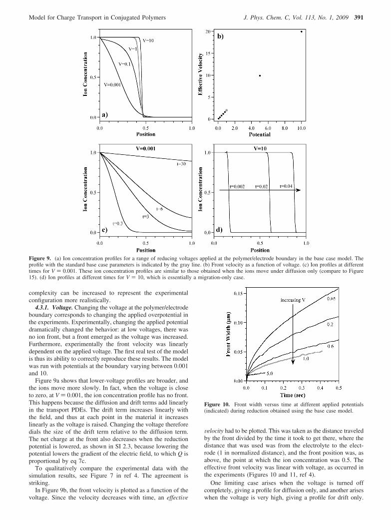
4.3.1. Voltage. Changing the voltage at the polymer/electrodeboundary corresponds to changing the applied overpotential inthe experiments. Experimentally, changing the applied potentialdramatically changed the behavior: at low voltages, there wasno ion front, but a front emerged as the voltage was increased.Furthermore, experimentally the front velocity was linearlydependent on the applied voltage. The first real test of the modelis thus its ability to correctly reproduce these results. The modelwas run with potentials at the boundary varying between 0.001and 10.

Figure 9a shows that lower-voltage profiles are broader, andthe ions move more slowly. In fact, when the voltage is closeto zero, at V ) 0.001, the ion concentration profile has no front.This happens because the diffusion and drift terms add linearlyin the transport PDEs. The drift term increases linearly withthe field, and thus at each point in the material it increaseslinearly as the voltage is raised. Changing the voltage thereforedials the size of the drift term relative to the diffusion term.The net charge at the front also decreases when the reductionpotential is lowered, as shown in SI 2.3, because lowering thepotential lowers the gradient of the electric field, to which Q isproportional by eq 7c.

To qualitatively compare the experimental data with thesimulation results, see Figure 7 in ref 4. The agreement isstriking.

In Figure 9b, the front velocity is plotted as a function of thevoltage. Since the velocity decreases with time, an effectiVe

Velocity had to be plotted. This was taken as the distance traveledby the front divided by the time it took to get there, where thedistance that was used was from the electrolyte to the elect-rode (1 in normalized distance), and the front position was, asabove, the point at which the ion concentration was 0.5. Theeffective front velocity was linear with voltage, as occurred inthe experiments (Figures 10 and 11, ref 4).

One limiting case arises when the voltage is turned offcompletely, giving a profile for diffusion only, and another ariseswhen the voltage is very high, giving a profile for drift only.

Figure 9. (a) Ion concentration profiles for a range of reducing voltages applied at the polymer/electrode boundary in the base case model. Theprofile with the standard base case parameters is indicated by the gray line. (b) Front velocity as a function of voltage. (c) Ion profiles at differenttimes for V ) 0.001. These ion concentration profiles are similar to those obtained when the ions move under diffusion only (compare to Figure15). (d) Ion profiles at different times for V ) 10, which is essentially a migration-only case.

Figure 10. Front width versus time at different applied potentials(indicated) during reduction obtained using the base case model.


(The potential cannot be set identically to zero in the model, soa very small value of V was used instead, V ) 0.001.) Underdiffusion only, ions initially enter the polymer rapidly (see t )0.3, Figure 9c), forming something like a front (i.e., the part ofthe film on the left is reduced and the part on the right isoxidized). A short time later, however, the polymer is partiallyreduced everywhere. The ion concentration at x ) 0 stays fixedat 1 by the boundary condition, and the level throughout therest of the polymer gradually rises. The polymer requires a longtime (t > 30) to become fully reduced. In the limiting case ofmigration only (V ) 10, Figure 9d), there is a definite front, onone side of which C ) 1 and on the other side of which C )0, that moves into the film. This front broadens very little overtime.

If the front broadening was due only to Fickian diffusion,then it would not depend on the potential. The front width as afunction of potential is shown in Figure 10, and there is a strongvoltage dependence. (The front broadening decreases ap-proximately as 1/�V, as shown in SI Figure SM5). This findingis in contradiction to the experimental data (Figure 13 in ref4), indicating that this base case model does not handle the frontbroadening properly.

The front broadening in the model is under the influence ofboth diffusion and migration. Diffusion tries to increase the frontwidth to lower the concentration gradient, while migrationdecreases the front width to lower the net charge. The migrationterm increases with the overpotential V, and the front broadeningis thus found to be slower, as expected.

4.3.2. Relationship between D and µ. Another, essentiallyequivalent, way to vary the relative contribution of the diffusionand migration terms in the base case model, in which thediffusivity and mobility are constant, is through their ratio. Thiswas set to D/µ ) 0.026 for both ions and holes in the basecase, where that value arose from assuming that the Einsteinrelation was valid. Increasing the ratio has the same effect aslowering the reduction potential (as shown in SI section 2.9).Also, as pointed out previously, since the density of ions (orholes) is so high in the fully reduced (oxidized) state that thecharges cannot realistically be considered to be noninteracting,the assumption that the Einstein relation is valid cannot be madeblindly, and the model must examine the effect of a varyingD/µ.

We therefore examined how varying the D/µ ratio based onthe more general relationship between diffusivity and mobilitygiven in eq 5 changed the concentration profiles. Specifically,Figure 11 shows the effect on the ion profile if DC/µC is

proportional to C. Since it is not clear how to choose themagnitude of this function to best compare with the base case,three relationships were used: (1) DC ) 0.026(1 + 5C), (2) DC

) 0.026(1 + 5C)/3.5, and (3) DC ) 0.026(1 + 5C)/6 (µC ) 1for all cases). The first gives the same minimum D/µ but anaveraged (over concentration) D/µ that is 6 times higher thanthe 0.026 of the base case; the second gives the same averageD/µ; and the third gives ∼2 times lower average D/µ but thesame maximum D/µ, thereby bracketing the base case. In Figure11, these three relationships are noted as higher, same, andlower, respectively.

For φ )-1, the speed of the front is not significantly changedby the alteration in DC/µC because front propagation speed isdominated by migration, so a variation in the diffusivity has anegligible effect. The front width is affected, however. For therelationship labeled “same av.”, the front is narrower thanthe base case, particularly at the foot where C is small. Thedifference between “same” and “lower” is also seen at the foot,becoming even sharper for the latter. For “higher”, the front isbroader everywhere. The same basic behavior was seen for φ

) 0.1. Thus, using a more general relationship between DC andµC only has a minor effect on the simulation predictions, andone that would be difficult to observe experimentally.

4.3.3. Finite Hole Mobility. Whether the electron movementor the hole movement is rate-limiting depends on their relativemobility. Experimental studies have suggested that hole transportis orders of magnitude faster.25-27 Even so, hole transport maybe the rate-limiting step in some experiments.28-31 The valueof adding eq 9b to the model, over our prior work in which ananalytical equation was used, is that it allows us to examinesuch cases.

The ion concentration profile resulting from setting the holemobility equal to the ion mobility is shown in Figure 12a incomparison with the base case, in which hole mobility was 1000times higher. (Additional ion concentration profiles can be foundin SI section 2.5.) The corresponding potentials as a functionof position are shown in Figure 12b.

The voltage profile changes significantly, now droppinglinearly between 0 and 1. This can, of course, be seen byexamining eq 10: since the conductivity and charge density ofthe oxidized and reduced regions are now identical, Ohm’s lawdictates a constant potential drop over the whole film. Theresulting smaller potential drop over the reduced regioncompared to the base case lowers the front velocity. The frontis also wider than in the base case since the electric field is

Figure 11. Ion concentration profiles in the base case model during reduction when DC/µC is not constant (base case, gray line) but proportionalto C (other lines). (a) V ) 1, t ) 0.12. (b) V ) 0.1, t ) 0.52.


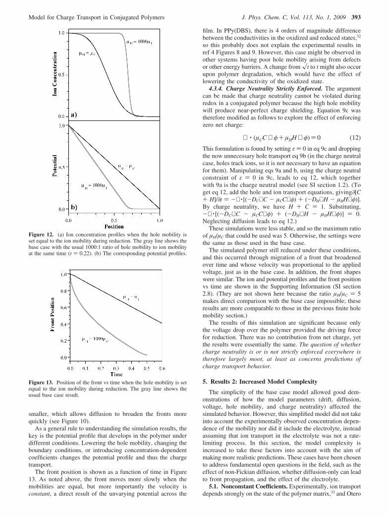
smaller, which allows diffusion to broaden the fronts morequickly (see Figure 10).

As a general rule to understanding the simulation results, thekey is the potential profile that develops in the polymer underdifferent conditions. Lowering the hole mobility, changing theboundary conditions, or introducing concentration-dependentcoefficients changes the potential profile and thus the chargetransport.

The front position is shown as a function of time in Figure13. As noted above, the front moves more slowly when themobilities are equal, but more importantly the velocity isconstant, a direct result of the unvarying potential across the

film. In PPy(DBS), there is 4 orders of magnitude differencebetween the conductivities in the oxidized and reduced states,32

so this probably does not explain the experimental results inref 4 Figures 8 and 9. However, this case might be observed inother systems having poor hole mobility arising from defectsor other energy barriers. A change from �t to t might also occurupon polymer degradation, which would have the effect oflowering the conductivity of the oxidized state.

4.3.4. Charge Neutrality Strictly Enforced. The argumentcan be made that charge neutrality cannot be violated duringredox in a conjugated polymer because the high hole mobilitywill produce near-perfect charge shielding. Equation 9c wastherefore modified as follows to explore the effect of enforcingzero net charge:

∇ · (µCC ∇ φ+ µHH ∇ φ)) 0 (12)

This formulation is found by setting ε ) 0 in eq 9c and droppingthe now unnecessary hole transport eq 9b (in the charge neutralcase, holes track ions, so it is not necessary to have an equationfor them). Manipulating eqs 9a and b, using the charge neutralconstraint of ε ) 0 in 9c, leads to eq 12, which togetherwith 9a is the charge neutral model (see SI section 1.2). (Toget eq 12, add the hole and ion transport equations, giving∂[C+ H]/∂t ) -∇ · [(-DC∇ C - µCC∇ φ) + (-DH∇ H - µHH∇ φ)].By charge neutrality, we have H + C ) 1. Substituting,-∇ · [(-DC∇ C - µCC∇ φ) + (-DH∇ H - µHH∇ φ)] ) 0.Neglecting diffusion leads to eq 12.)

These simulations were less stable, and so the maximum ratioof µH/µC that could be used was 5. Otherwise, the settings werethe same as those used in the base case.

The simulated polymer still reduced under these conditions,and this occurred through migration of a front that broadenedover time and whose velocity was proportional to the appliedvoltage, just as in the base case. In addition, the front shapeswere similar. The ion and potential profiles and the front positionvs time are shown in the Supporting Information (SI section2.8). (They are not shown here because the ratio µH/µC ) 5makes direct comparison with the base case impossible; theseresults are more comparable to those in the previous finite holemobility section.)

The results of this simulation are significant because onlythe voltage drop over the polymer provided the driving forcefor reduction. There was no contribution from net charge, yetthe results were essentially the same. The question of whethercharge neutrality is or is not strictly enforced eVerywhere istherefore largely moot, at least as concerns predictions ofcharge transport behaVior.

5. Results 2: Increased Model Complexity

The simplicity of the base case model allowed good dem-onstrations of how the model parameters (drift, diffusion,voltage, hole mobility, and charge neutrality) affected thesimulated behavior. However, this simplified model did not takeinto account the experimentally observed concentration depen-dence of the mobility nor did it include the electrolyte, insteadassuming that ion transport in the electrolyte was not a rate-limiting process. In this section, the model complexity isincreased to take these factors into account with the aim ofmaking more realistic predictions. These cases have been chosento address fundamental open questions in the field, such as theeffect of non-Fickian diffusion, whether diffusion-only can leadto front propagation, and the effect of the electrolyte.

5.1. Nonconstant Coefficients. Experimentally, ion transportdepends strongly on the state of the polymer matrix,33 and Otero

Figure 12. (a) Ion concentration profiles when the hole mobility isset equal to the ion mobility during reduction. The gray line shows thebase case with the usual 1000:1 ratio of hole mobility to ion mobilityat the same time (t ) 0.22). (b) The corresponding potential profiles.

Figure 13. Position of the front vs time when the hole mobility is setequal to the ion mobility during reduction. The gray line shows theusual base case result.


et al.21 have developed a very successful polymer conformationalrelaxation model to predict peak positions in chronoampero-grams that takes the state of the matrix into account. Thus, ourmodel needed to have a mechanism for handling non-Fickiandiffusion. One way that non-Fickian diffusion has been dealtwith in the literature (albeit with varying degrees of success)hasbeenthroughaconcentration-dependentdiffusioncoefficient.34,35

In this section, we explore the consequences of taking thisapproach.

5.1.1. Background. There are numerous models for diffusionof solutes in polymers, as reviewed, for example, by Masaro etal.36 In most of the models, the diffusion coefficient is of theform D ) D0e-something, where the exponent might be related tothe polymer volume fraction, the radius of the diffusing species,a screening parameter, a concentration, a free volume, anactivation energy, etc. The model that has been found to be themost applicable to aqueous electrolytes (as opposed to organicspecies or gases) diffusing in hydrated polymers (as opposedto polymer solutions or gels) is based on work by Yasuda37

and assumes that diffusion depends on free volume, which hasits primary contribution from the water in the polymer

D ≈ D0e-(V*⁄HVf,H2O) (13)

where V* depends on the size of the diffusant; H is the hydration,or volume fraction of water, in the polymer; and Vf,H2O is thewater free volume. This model assumes no interactions betweenthe diffusing species and the polymer and does not take intoaccount temperature effects. A more complex model by Vrentasand Duda does include these effects but has 14 parameters, mostof which are unknown.36 Neither model takes into accountincreasing polymer volume with penetration of the diffusant.Another free volume model, by Peppas and Reinhart, wasdesigned to apply to cross-linked polymers36

D)D0P� e-kRh

2

Q-1 (14)

where P� is related to the mesh size of the gel; k is related tothe polymer; Rh is the hydrodynamic radius of the particle; andQ is the volume degree of swelling. This model also does nottake into account interactions between ionized diffusants andthe polymer. Models that consider migration have usuallyassumed the Einstein relation to be valid. There are no modelsthat take into account all of the following factors in PPy(DBS):polymer cross-linking; volume increase upon water and ion

ingress; interactions between ions and polymer, ions and solvent,and solvent and polymer; effective ion size and charge; andchain conformational changes. Masaro et al. concluded that itstill remains virtually impossible to estimate or predict thediffusion coefficient for any particular system under specificconditions.

5.1.2. Approach to Non-Fickian DiffusiWity. It must beemphasized that to properly handle polymer relaxation effectsa mechanical model needs to be incorporated into our transportmodel, which will be the subject of future work. Nevertheless,it is of value to study the incorporation of a rudimentarymechanism to make diffusion non-Fickian.

We based our coefficient dependence on empirical data fromref 4 (Figure 15). We had shown that the front velocity, V, vsthe total charge consumed, Qtot, could be reasonably well fitwith

V ∼ e2Qtotal (15)

but that the front velocity vs the charge associated with strain,Qstrain, (under Gaussian 1) had a different relationship and waslinear

V ∼ Qstrain (16)

On the basis of the data in ref 4, eq 16 is the one that morecorrectly describes the relationship, but since eq 15 has astronger dependence on Q (which is equal to C in this paper),it will better display any changes in model behavior as a resultof making the coefficients nonconstant. Therefore, this was therelationship used here. Assuming the usual proportionality ofthe ion velocity to the electric field strength and the mobility,V ) µE, and assuming that the electronic charge is equal to thenumber of cations exchanged, we can write the mobility in theform

µC ) µ0e2C (17)

Maintaining the link between diffusivity and mobility that wasimposed in the base case, D/µ ) 0.026, gives the diffusivitythe same dependence as the mobility

DC )D0e2C (18)

This form for the coefficients is analogous to eqs 13 and 14.The PDE for holes was left unaltered (since hole transport isnot the rate-limiting step and also because its dependence on Cis unknown), and no other changes were made to eq 9. We rantwo scenarios. In the first, drift was included, and in the second,only diffusion was considered. The former was expected to giveresults that agreed more closely with our experiments than thebase case with constant coefficients.

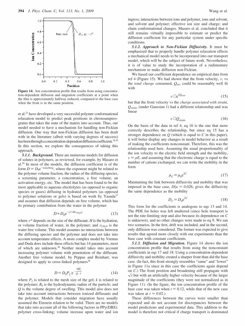
5.1.3. Diffusion and Migration. Figure 14 shows the ionconcentration profile that results from using the nonconstantcoefficients in eqs 17 and 18. Using a concentration-dependentdiffusivity and mobility created a sharper front than did the basecase. (In fact, this front strongly resembles “same” and “lower”in Figure 11a since in this case the coefficients again dependon C.) The front position and broadening still propagate with�t but with an artificially higher velocity because of the largermagnitude of the coefficients (they were not normalized as inFigure 11). (In the figure, the ion concentration profile of thebase case was taken when t ) 0.12, while that of the new casewas taken at t ) 0.02.)

These differences between the curves were smaller thanexpected and do not account for discrepancies between themodel predictions and experimental data. This addition to themodel is therefore not critical if charge transport is dominated

Figure 14. Ion concentration profile that results from using concentra-tion-dependent diffusion and migration coefficients at a point whenthe film is approximately halfway reduced, compared to the base casewhen the front is in the same position.


by migration. We include it, however, in all the sections thatfollow, unless otherwise noted, because we know with certaintyfrom experimental results that diffusion in these systems is notFickian. Nevertheless, we can conclude that this method ofhandling non-Fickian diffusion is unsuitable for PPy(DBS) andprobably for other conjugated polymers as well.

5.1.4. Diffusion Only. In a second case run with nonconstantcoefficients, the migration term in eq 9b was removed so thatthe ion transport PDE had only a diffusion term. The motivationfor simulating this case was to determine the form of thedependence of DC on C that would be needed to produce a frontin the absence of migration. Lacroix et al.5 had previously shownthat a hole diffusivity DH that increased steeply with theconcentration of oxidized sites could lead to a moving front,and for completeness we now did this for ion diffusivity.Furthermore, this case is of interest because a number of theorieshave assumed that charge moves only due to diffusion. Finally,it is of interest to see whether the experimental results couldarise due to ESCR effects (handled here indirectly through theconcentration-dependent diffusion coefficient) combined withtransport solely by ion diffusion. Once again, only the diffusivityof the ions was made concentration dependent, and the PDEfor holes was left unaltered.

Figure 15 shows ion concentration profiles for three relation-ships between diffusivity and ion concentration: a linearrelationship (as in eq 16)

DC )D0(1+ 5C) (19)

the exponential relationship in eq 18, and an even steeperexponential relationship

DC )D0e5C (20)

The linear relationship was designed to have the same diffusivityas eq 18 at an ion concentration of 1.

The linear relationship, unsurprisingly, produces no front inthe event that transport is by diffusion alone. The experimentalrelationship DC ∼ e2C, however, results in a curve with aninflection point, which is thus quasi-frontlike. The very steepexponential relationship of eq 20 produces even more of afrontlike shape, and its position advances with the square rootof time. However, since there is no migration in this model,the front velocity is independent of the voltage and so does not

match the experimental results. This lack of a dependence onV arises because the electrolyte is not yet included in the model.

Of these curves, it is actually the base case, with DC )constant, and the linear case that most closely resemble theexperimental color profiles at low voltage (compare Figure 7in ref 4). This may indicate that the linear dependence on C ismore appropriate than the exponential, consistent with the chargeassociated with strain rather than the total charge. Alternatively,it may indicate that the form of the diffusion term in the modelis fundamentally incorrect. Rather, a different method ofhandling the non-Fickian diffusion may be needed to correctlymodel transport at low V, such as including chain conformationalchanges, elastic energies, or changes in modulus with doping.

5.2. Addition of the Electrolyte. The next step in increasingmodel complexity was to add ion transport within the electrolyte,retaining the nonconstant coefficients. With this addition, themodel was as complete as it could be made based only on chargetransport PDEs and the Poisson equation. We therefore refer tothis as the “full model” and use it in later papers to examinehow changes in the polymer or the experimental configurationchange the ion transport behavior.

In the model up to this point, the same voltage drop wasimposed across the polymer throughout the reduction process,regardless of whether it was oxidized, and thus highly conduc-tive, or reduced and highly resistive. In reality, however, thepotential is instead dropped across the electrolyte when thepolymer is conductive. Considering the polymer and the elec-trolyte as if they behave as two resistors in series, the potentialacross the polymer (which has a variable resistance) dependson the magnitude of its resistance versus that of the electrolytethrough a simple voltage-divider relation. Thus, this full modelwas expected to give more accurate predictions of the electricfields in the film, which translates directly to better predictionsof ion profiles and front velocities vs time.

Another reason that it was important to add the electrolytewas to examine the effect of ion depletion and ion double-layerbuildup at the polymer/electrolyte boundary. It has beenpostulated that even if ion transport is by diffusion only, a highion concentration in the double layer may account for theobserved faster redox speeds with higher applied voltages(diffusive elastic metal model38). This could only be investigatedby the addition of the electrolyte.

5.2.1. Full Model. The electrolyte was added as a secondmaterial, as illustrated in Figure 16. Charge transport in theelectrolyte was governed by the following PDEs. These areessentially identical to those used in polymer, but instead ofholes, eq 22 accounts for the anions, and the net charge in eq23 is simply given by the difference between the anion andcation concentrations at a given location. Convection, which issmall in unstirred solutions, was not included in the electrolytemodel.

∂Ce

∂t)- ∇ · (-DCe ∇ Ce - µCeCe ∇ φ) (21)

∂A∂t

)- ∇ · (-DA ∇ A+ µAA ∇ φ) (22)

εo ∇ (εe ∇ φ))Q)Ce -A (23)

Here Ce is the cation concentration in the electrolyte; A is theanion concentration in the electrolyte; DCe is the diffusivity;µCe is the mobility of the cation in the electrolyte; DA is thediffusivity and µA is the mobility of the anion in the electrolyte;and εe is the dielectric constant of the electrolyte. The iondiffusivity and mobility in the polymer are as given by eqs 17and 18.

Figure 15. Ion concentration profiles resulting from three concentra-tion-dependent ion diffusivities when ion transport is solely by diffusionduring reduction. The diffusion-only case with constant coefficients isshown for comparison (gray line).


As in the previous section, we began with a starting pointcase. Both anions and cations were treated as singly charged.In the electrolyte, the cations were assumed to have a 10×higher mobility than the anions (Figure 16a) since in ourexperiments the Na+ is much smaller than the DBS-. The cationmobility in the electrolyte was assumed to be 1000 times higherthan in the polymer, based on reported diffusivity values in theliterature.39,40 The Einstein relation was assumed to be valid,and the dielectric constant of the electrolyte was set to the samevalue as that for the polymer. The electrolyte was set to be 10×longer than the polymer, based on our experimental configu-ration. The parameters in the polymer were the same as thoseused in the base case, except for the implementation ofnonconstant coefficients.

There were three boundaries in the new model (Figure 16c).On the left-hand side (x )-10) is a second electrode, equivalentto an experimental configuration in which the counter andreference electrodes are shorted. At this electrode/electrolyteboundary, the anion and cation concentrations were set equalto the salt concentration in the bulk of the electrolyte. Sincewe used a 0.1 M electrolyte concentration for the experiments,this was also used in the model system (equal to 0.033Co, sinceCmax ) 3 M). The potential at that boundary was zero duringthe reduction process. The interface between the electrolyte andthe polymer (x ) 0) had a no-flux condition for anions andholes, keeping them confined in the electrolyte and polymer,respectively. Lastly, the polymer/electrode interface (x ) 1) hadthe same boundary conditions as in the base case.

In the initial conditions for the simulation, anion and cationconcentrations throughout the electrolyte were equal to 0.033Co.In the polymer, the initial conditions were the same as used inthe base case: C ) 0 and H ) 1.

5.2.2. Full Model Results. The concentrations of the chargedspecies are shown in Figure 17a when the front has reachedhalfway into the polymer. In the new electrolyte region, bothanions and cations are depleted near the surface of the polymer,their concentrations returning to bulk values by x ) -4. Just atthe interface, though, the cation concentration rises steeply,forming a thin double-layer (more clearly seen in the inset ofFigure 17a). The profiles in the polymer are qualitatively similarto those in the base case.

The electric field (Figure 17b), which is Eb ) -∇ φ ) -dφ/dx in this 1-D case, creates a sharp build-up of cations in theelectrolyte (Ce) at the electrolyte/polymer boundary; i.e., thecations form a double-layer. The reason for this is that the ionmigration flux is the product of three terms: ion mobility, ionconcentration, and electric field (eq 21). The electric field isnearly zero in the bulk of the electrolyte (on the left), becomeshigh near the electrolyte/polymer boundary, drops to a low valuein the reduced part of the polymer, and returns to almost zeroin the conducting region. The ion concentration in the bulk ofthe electrolyte is ∼30 times lower than in the reduced polymer,but the mobility is 1000 times larger (see Figure 16 and Figure17). Thus, the flux in the electrolyte near the polymer (µCeCeE) very high × low × very high) is far greater than in thereduced part of the polymer (µCCE ) low × high × low). Thefaster arrival of cations at the boundary than they can be takenup by the polymer causes the pile-up of ions at the interface.Diffusion, which opposes such concentration gradients, limitsthe size of this double-layer.

The rapid supply of cations to the electrolyte/polymerboundary further creates a cation depletion region to the left ofthe boundary, within the region -2 < x < -0.1, as seen in theinset of Figure 17. The flux in the bulk of the electrolyte, becauseof the small E field there, cannot keep up with the supply ofions to the double-layer. There is also a depletion of anionsnear the interface, caused directly by the electric field, whichattracts the cations but repels the anions.

The potential as a function of position is shown at three timesnapshots in Figure 17b. Initially, when the polymer is in itsconducting, oxidized state, all of the voltage is applied acrossthe electrolyte. As the polymer is reduced, the potential acrossit rises, but even so, halfway through the reduction process ap-proximately 70% of the potential drop is still across theelectrolyte. The largest part of this drop occurs across thedepletion and double layer regions. The profile does not changesignificantly thereafter: at the end of the process, only slightlymore of the potential is dropped across the polymer.

The front position moves as �t in the polymer (shown inthe Supporting Information, section 3.3), just as it did in thebase case. This is because after an initial rapid increase, up tot ) 0.01, the potential across the polymer grows only slowly.(The potential drop across the polymer over time is shown inSI section 3.2). Therefore, the behavior is, as in the base case,dominated by the change in width of the conducting region asthe front moves forward. The front also still broadens as �t.(This is also shown in the SI, section 3.3.) In addition, theeffective front velocity is still linearly proportional to the appliedpotential. Regardless of the size of the applied voltage, thismodel did not show a limiting front velocity due to transport inthe electrolyte.

The small differences in behavior between this full modeland the previous one, in section 5.1, stems from the fact thatpotential drop across the electrolyte is substantial, particularlyacross the depletion layer. This lowers the migration term inthe polymer. If the potentials across the polymer in the twomodels are equal, approximated by using a value of V ) 0.25in the base case, the two produce essentially identical results(see SI section 3.3).

5.2.3. Variation: Diffusion Only. Because of the continueddiscussion in the literature maintaining that ion transport is dueonly to diffusion, this question was examined once again usingthe full model. In the diffusive elastic metal model,38 the forcefor ion transport into the polymer is a high concentration ofions in the double layer at the polymer/electrolyte interface, and

Figure 16. (a) Parameters, (b) PDEs, and (c) boundary conditions usedduring reduction in the full model, a 1-D model that includes theelectrolyte and nonconstant coefficients.


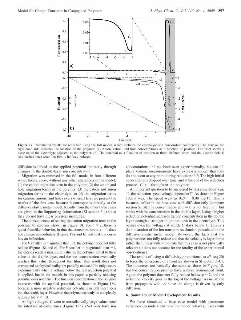
diffusion is linked to the applied potential indirectly throughchanges in the double-layer ion concentration.

Migration was removed in the full model in four differentways, taking away, without any other alterations in the model,(1) the cation migration term in the polymer, (2) the cation andhole migration terms in the polymer, (3) the cation and anionmigration terms in the electrolyte, or (4) the migration termsfor cations, anions, and holes everywhere. Here, we present theresults of the first case because it corresponds directly to thediffusive elastic metal model. Results from the other three casesare given in the Supporting Information (SI section 3.4) sincethey do not have clear physical meanings.

The consequences of setting the cation migration term in thepolymer to zero are shown in Figure 18. For t < 2, there isquasi-frontlike behavior, in that the concentration at x ) 1 doesnot change immediately (Figure 18a and b) and that the curvehas an inflection.

For V smaller in magnitude than -2, the polymer does not fullyreduce (Figure 18a and c). For V smaller in magnitude than -1,the cations reach a maximum value in the polymer equal to theirvalue in the double layer, and the ion concentration eventuallyreaches this value throughout the film. This result does notcorrespond to physical reality. (A partially reduced film only occursexperimentally when a voltage below the full reduction potentialis applied, but in the models in this paper, a partially reducingpotential does not exist.) The final ion concentration in the polymerincreases with the applied potential, as shown in Figure 18c,because a more negative reduction potential can pull more ionsinto the double layer. However, the polymer can only be completelyreduced for V > 10.

At high voltages, C went to unrealistically large values nearthe interface at early times (Figure 18b). (Not only have ion

concentrations >1 not been seen experimentally, but out-of-plane volume measurements have expressly shown that theydo not occur at any point during reduction.33,41) The high initialconcentrations dropped over time, and at the end of the reductionprocess, C ≈ 1 throughout the polymer.

An important question to be answered by this simulation was,“Is the reduction speed voltage-dependent?”. As shown in Figure18d, it was. The speed went as 0.24 + 0.08 log(V). This isbecause, unlike in the base case with diffusion-only (comparesection 5.1.4), the concentration at x ) 0 is not fixed at 1 butvaries with the concentration in the double layer. Using a higherreduction potential increases the ion concentration in the doublelayer through a stronger migration term in the electrolyte. Thisoccurs even for voltages at which C stays below 1. This is ademonstration of the ion transport mechanism postulated in thediffusive elastic metal model. However, the facts that thepolymer does not fully reduce and that the velocity is logarithmicrather than linear with V indicate that this case is not physicallyrelevant (it does not account for the totality of the experimentalobservations).

The results of using a diffusivity proportional to e5C (eq 20)to force the emergence of a front are shown in SI section 3.4.1.The outcomes are basically the same as those in Figure 18,but the concentration profiles have a more pronounced front.Again, the polymer does not fully reduce below φ ∼ 2, and thereduction velocity goes as the log of the voltage. As usual, thefront propagates with �t since the charge is driven by onlydiffusion.

6. Summary of Model Development Results

We have simulated a base case model with parametervariations (to understand how the model behaves), cases with

Figure 17. Simulation results for reduction using the full model, which includes the electrolyte and nonconstant coefficients. The gray on theright-hand side indicates the location of the polymer. (a) Anion, cation, and hole concentrations as a function of position. The inset shows aclose-up of the electrolyte adjacent to the polymer. (b) The potential as a function of position at three different times and the electric field E(dot-dashed line) when the film is halfway reduced.


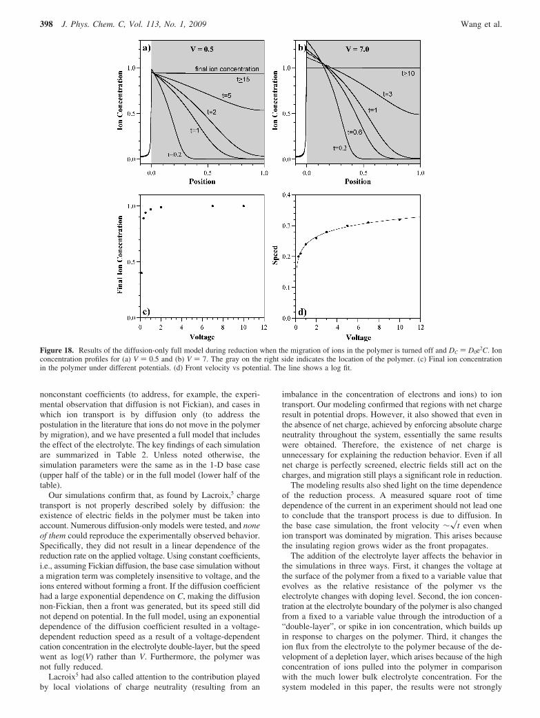
nonconstant coefficients (to address, for example, the experi-mental observation that diffusion is not Fickian), and cases inwhich ion transport is by diffusion only (to address thepostulation in the literature that ions do not move in the polymerby migration), and we have presented a full model that includesthe effect of the electrolyte. The key findings of each simulationare summarized in Table 2. Unless noted otherwise, thesimulation parameters were the same as in the 1-D base case(upper half of the table) or in the full model (lower half of thetable).

Our simulations confirm that, as found by Lacroix,5 chargetransport is not properly described solely by diffusion: theexistence of electric fields in the polymer must be taken intoaccount. Numerous diffusion-only models were tested, and noneof them could reproduce the experimentally observed behavior.Specifically, they did not result in a linear dependence of thereduction rate on the applied voltage. Using constant coefficients,i.e., assuming Fickian diffusion, the base case simulation withouta migration term was completely insensitive to voltage, and theions entered without forming a front. If the diffusion coefficienthad a large exponential dependence on C, making the diffusionnon-Fickian, then a front was generated, but its speed still didnot depend on potential. In the full model, using an exponentialdependence of the diffusion coefficient resulted in a voltage-dependent reduction speed as a result of a voltage-dependentcation concentration in the electrolyte double-layer, but the speedwent as log(V) rather than V. Furthermore, the polymer wasnot fully reduced.

Lacroix5 had also called attention to the contribution playedby local violations of charge neutrality (resulting from an

imbalance in the concentration of electrons and ions) to iontransport. Our modeling confirmed that regions with net chargeresult in potential drops. However, it also showed that even inthe absence of net charge, achieved by enforcing absolute chargeneutrality throughout the system, essentially the same resultswere obtained. Therefore, the existence of net charge isunnecessary for explaining the reduction behavior. Even if allnet charge is perfectly screened, electric fields still act on thecharges, and migration still plays a significant role in reduction.

The modeling results also shed light on the time dependenceof the reduction process. A measured square root of timedependence of the current in an experiment should not lead oneto conclude that the transport process is due to diffusion. Inthe base case simulation, the front velocity ∼�t even whenion transport was dominated by migration. This arises becausethe insulating region grows wider as the front propagates.

The addition of the electrolyte layer affects the behavior inthe simulations in three ways. First, it changes the voltage atthe surface of the polymer from a fixed to a variable value thatevolves as the relative resistance of the polymer vs theelectrolyte changes with doping level. Second, the ion concen-tration at the electrolyte boundary of the polymer is also changedfrom a fixed to a variable value through the introduction of a“double-layer”, or spike in ion concentration, which builds upin response to charges on the polymer. Third, it changes theion flux from the electrolyte to the polymer because of the de-velopment of a depletion layer, which arises because of the highconcentration of ions pulled into the polymer in comparisonwith the much lower bulk electrolyte concentration. For thesystem modeled in this paper, the results were not strongly

Figure 18. Results of the diffusion-only full model during reduction when the migration of ions in the polymer is turned off and DC ) D0e2C. Ionconcentration profiles for (a) V ) 0.5 and (b) V ) 7. The gray on the right side indicates the location of the polymer. (c) Final ion concentrationin the polymer under different potentials. (d) Front velocity vs potential. The line shows a log fit.


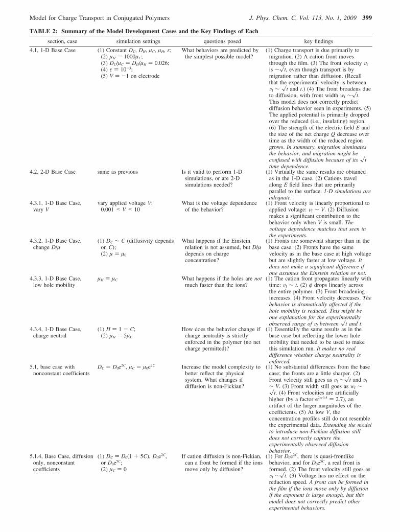
TABLE 2: Summary of the Model Development Cases and the Key Findings of Each

section, case simulation settings questions posed key findings

4.1, 1-D Base Case (1) Constant DC, DH, µC, µH, ε;(2) µH ) 1000µC;(3) DC/µC ) DH/µH ) 0.026;(4) ε ) 10-3;(5) V ) -1 on electrode

What behaviors are predicted bythe simplest possible model?

(1) Charge transport is due primarily tomigration. (2) A cation front movesthrough the film. (3) The front velocity Vf

is ∼�t, even though transport is bymigration rather than diffusion. (Recallthat the experimental velocity is betweenVf ∼ �t and t.) (4) The front broadens dueto diffusion, with front width wf ∼�t.This model does not correctly predictdiffusion behavior seen in experiments. (5)The applied potential is primarily droppedover the reduced (i.e., insulating) region.(6) The strength of the electric field E andthe size of the net charge Q decrease overtime as the width of the reduced regiongrows. In summary, migration dominatesthe behaVior, and migration might beconfused with diffusion because of its �ttime dependence.

4.2, 2-D Base Case same as previous Is it valid to perform 1-Dsimulations, or are 2-Dsimulations needed?

(1) Virtually the same results are obtainedas in the 1-D case. (2) Cations travelalong E field lines that are primarilyparallel to the surface. 1-D simulations areadequate.

4.3.1, 1-D Base Case,vary V

vary applied voltage V:0.001 < V < 10

What is the voltage dependenceof the behavior?

(1) Front velocity is linearly proportional toapplied voltage: Vf ∼ V. (2) Diffusionmakes a significant contribution to thebehavior only when V is small. TheVoltage dependence matches that seen inthe experiments.

4.3.2, 1-D Base Case,change D/µ

(1) DC ∼ C (diffusivity dependson C);(2) µ ) µ0

What happens if the Einsteinrelation is not assumed, but D/µdepends on chargeconcentration?

(1) Fronts are somewhat sharper than in thebase case. (2) Fronts have the samevelocity as in the base case at high voltagebut are slightly faster at low voltage. Itdoes not make a significant difference ifone assumes the Einstein relation or not.

4.3.3, 1-D Base Case,low hole mobility

µH ) µC What happens if the holes are notmuch faster than the ions?

(1) The cation front propagates linearly withtime: Vf ∼ t. (2) φ drops linearly acrossthe entire polymer. (3) Front broadeningincreases. (4) Front velocity decreases. ThebehaVior is dramatically affected if thehole mobility is reduced. This might beone explanation for the experimentallyobserVed range of Vf between �t and t.

4.3.4, 1-D Base Case,charge neutral

(1) H ) 1 - C;(2) µH ) 5µC

How does the behavior change ifcharge neutrality is strictlyenforced in the polymer (no netcharge permitted)?

(1) Essentially the same results as in thebase case but reflecting the lower holemobility that needed to be used to makethis simulation run. It makes no realdifference whether charge neutrality isenforced.

5.1, base case withnonconstant coefficients

DC ) D0e2C, µC ) µ0e2C Increase the model complexity tobetter reflect the physicalsystem. What changes ifdiffusion is non-Fickian?

(1) No substantial differences from the basecase; the fronts are a little sharper. (2)Front velocity still goes as Vf ∼�t and Vf

∼ V. (3) Front width still goes as wf ∼�t. (4) Front velocities are artificiallyhigher (by a factor e2×0.5 ) 2.7), anartifact of the larger magnitudes of thecoefficients. (5) At low V, theconcentration profiles still do not resemblethe experimental data. Extending the modelto introduce non-Fickian diffusion stilldoes not correctly capture theexperimentally obserVed diffusionbehaVior.

5.1.4, Base Case, diffusiononly, nonconstantcoefficients

(1) DC ) D0(1 + 5C), D0e2C,or D0e5C;(2) µC ) 0

If cation diffusion is non-Fickian,can a front be formed if the ionsmove only by diffusion?

(1) For D0e2C, there is quasi-frontlikebehavior, and for D0e5C, a real front isformed. (2) The front velocity still goes asVf ∼�t. (3) Voltage has no effect on thereduction speed. A front can be formed inthe film if the ions moVe only by diffusionif the exponent is large enough, but thismodel does not correctly predict otherexperimental behaViors.


affected by these alterations or, as mentioned previously, bythe use of nonconstant coefficients. In fact, the only significantdifference arose during the diffusion-only case, where the basecase model showed no dependence of the reduction speed onapplied voltage, and because of the introduction of the double-layer, the full model did. Thus, it is not necessary to use anythingmore elaborate than the base case model to describe reductionof covered films of PPy(DBS).

Nevertheless, we shall use the full model in subsequent papersboth because it incorporates more realistic physics and becauseit turns out to be necessary for other geometries, materials, andconditions, such as encountered when examining the effect ofelectrolyte concentration. In fact, we show in the next paperthat inclusion of the electrolyte can dramatically change thepredicted behavior and is necessary for understanding thin films.

7. Discussion and Conclusions

The contributions of this study were choosing equations,boundary conditions, and numerical methods that were consis-tent with the known physics and thereby obtaining results thatwere consistent with experimental measurements. This first-principles approach allowed us to address a broad range of issues(effects of parameter variations, diffusion that is not Fickian,transport by diffusion only, the effect of the electrolyte).

The technical details of the system made the simulationschallenging. We took advantage of the full suite of modelingtricks: we used symmetry to reduce model complexity, intro-duced scaling to handle disparities in dimension (e.g., 1:500aspect ratios in film thickness to width), used limiting behavior

to disregard some parameters (e.g., too large dielectric con-stants), rounded corners (e.g., in the film, in ion concentrations)to avoid singularities; meshed more tightly in regions of rapidchange, etc.

Given the simplicity of the charge transport model presentedin this paper, it did remarkably well in predicting the reductionprocess in PPy(DBS). It has thus allowed us to answer severalimportant questions that have long been debated in the literature.The first question was, does migration contribute to ion transportin conjugated polymers? This question is fundamental since itinvolves the basic driving mechanism in devices and thusimpacts how they can be controlled. The results unambiguouslyshow that migration must be included since none of the manydiffusion-only models that were examined could account forthe experimental observations. The behavior switches fromdiffusion-dominated at small overpotentials to migration-dominated at higher voltages. In the latter cases, the behavioris determined largely by where the voltage drops occur in thesystem. A second question was, is there a net charge in thepolymer? The simulations show that this question is basicallyirrelevant: the presence or absence of a net charge makes noreal difference to the results.

The model also revealed some surprises, such as thatmigration can lead to �t time dependences. Previously,experimental results with this time dependence were automati-cally attributed to diffusion, regardless of the fact that diffusionshould not have been expected to be Fickian in these systems.

The model did not account for all of the results, however: itfailed to correctly predict the front broadening behavior despite

TABLE 2: Continued

section, case simulation settings questions posed key findings

5.2.2, Full Model (1) DC ) D0e2C, µC ) µ0e2C;(2) New anion, cation PDEs inan electrolyte layer;(3) New boundary conditions,including φ ) 0 at the edge ofthe electrolyte

Increase the model complexity tobetter reflect the physicalsystem. How is the behavioraffected by including thepotential drops and ion transportin the electrolyte?

(1) There is a significant voltagedrop across the electrolyte. Atthe end of the reduction process,only ∼30% of the voltage dropis across the insulating polymer.(2) Depletion and double layersform in the electrolyte. (3) Frontvelocity still goes as Vf ∼ �tand Vf ∼ V. (4) If we set V )0.25 across the polymer in thebase case (thereby mimicking a75% voltage drop across theelectrolyte), the resulting chargeprofiles and front velocity arevirtually identical to those in thefull model. Under theseconditions, the behaVior uponincluding the electrolyte is thesame as in the base case aftertaking into account the resistiVepotential drop oVer theelectrolyte.

5.2.3, Full Model,diffusion only

(1) DC ) D0e2C; (2) µC ) 0 How is non-Fickiandiffusion-only cation transportaffected by the inclusion of anelectrolyte layer?

(1) The cation concentration inthe polymer equals the cationconcentration in the electrolytedouble-layer. (2) The polymerdoes not fully reduce unlessextreme voltages are applied (Vg 10). (3) Quasi-frontlikebehavior is again seen. (4) Thereduction speed does depend onvoltage, but the dependence isweak, going as log(V). Adiffusion-only model does notcorrectly predict theexperimental behaVior.


the fact that the diffusion was treated using an accepted approachfor modeling non-Fickian diffusion. We conclude that to do thisfuture models need to include polymeric and/or electrochemicalcontributions to the transport.

Acknowledgment. We would like to acknowledge theLaboratory for Physical Sciences and the Dupont YoungProfessor Award for supporting this work. We thank the Comsoltechnical staff for helping us to solve several simulation issues.We also thank Kevin Lewy, Mario Urdaneta, Jason West, andPramod Mathai for assistance with our simulation server.

Supporting Information Available: Includes additionalsimulation results, including more detailed derivations, theeffects of varying parameters such as the dielectric constant,and further charge-neutrality and diffusion-only cases. Thismaterial is available free of charge via the Internet at http://pubs.acs.org.

References and Notes

(1) Albery, W. J.; Mount, A. R. Transmission-line model for conductingpolymers including cations and Donnan exclusion. J. Chem. Soc., FaradayTrans. 1993, 89 (14), 2487–2497.

(2) Fletcher, S. Contribution to the theory of conducting-polymerelectrodes in electrolyte solutions. J. Chem. Soc., Faraday Trans. 1993, 89(2), 311–320.

(3) Wang, X.; Smela, E. Color and volume change in PPy(DBS). J.Phys. Chem. C 2009, 113, 359-368.

(4) Wang, X.; Smela, E. Experimental studies of ion transport inPPy(DBS) J. Phys. Chem. C 2009, 113, 369-381.

(5) Lacroix, J. C.; Fraoua, K.; Lacaze, P. C. Moving front phenomenain the switching of conductive polymers. J. Electroanal. Chem. 1998, 444(1), 83–93.

(6) Berthier, F.; Diard, J.-P.; Montella, C. Numerical solution of coupledsystems of ordinary and partial differential equations. Application to thestudy of electrochemical insertion reactions by linear sweep voltammetry.J. Electroanal. Chem. 2001, 502, 126–131.

(7) Deiss, E.; Haas, O.; Schlenoff, J. B. Numerical-simulation of thecyclic voltammogram of polyacetylene. J. Electrochem. Soc. 1995, 142 (10),3256–3262.

(8) Bisquert, J.; Vikhrenko, V. S. Analysis of the kinetics of ionintercalation. Two state model describing the coupling of solid state iondiffusion and ion binding processes. Electrochim. Acta 2002, 47 (24), 3977–3988.

(9) Wang, X.; Shapiro, B.; Smela, E. Visualizing ion transport inconjugated polymers. AdV. Mater. 2004, 16 (18), 1605–1609.

(10) Wang, X.; Shapiro, B.; Smela, E. Modeling charge transport inconjugated polymers; SPIE 13th Annual Int’l. Symposium on SmartStructures and Materials, EAPAD, San Diego, CA, 2006.

(11) Bard, A. J.; Faulkner, L. R. Electrochemical Methods: Fundamen-tals and Applications, 2nd ed.; John Wiley & Sons, Inc.: New York, 2001.

(12) Bay, L.; Jacobsen, T.; Skaarup, S.; West, K. Mechanism of actuationin conducting polymers: osmotic expansion. J. Phys. Chem. B 2001, 105(36), 8492–8497.

(13) Streetman, B. G.; Banerjee, S. Solid State Electronic DeVices, 5thed.; Prentice-Hall: Upper Saddle River, 2000.

(14) Smela, E. Microfabrication of PPy microactuators and otherconjugated polymer devices. J. Micromech. Microeng. 1999, 9, 1–18.

(15) Schey, H. M. DiV, Grad, Curl, and All That: An Informal Text onVector Calculus; W. W. Norton & Company: New York, 1973.

(16) Ashcroft, N. W.; Mermin, N. D. Solid State Physics; SaundersCollege: Philadelphia, 1976.

(17) Guidoni, S. E.; Aldao, C. M. On diffusion, drift and the Einsteinrelation. Eur. J. Phys 2002, 23, 395–402.

(18) Feynman, R. P.; Leighton, R. B.; Sands, M. The Feynman Lectureson Physics; Addison-Wesley Publishing Company, 1964.

(19) Roichman, Y.; Tessler, N. Generalized Einstein relation fordisordered semiconductorssimplications for device performance. Appl.Phys. Lett. 2002, 80 (11), 1948–1950.

(20) Panton, R. L. Incompressible Flow, 2nd ed.; John Wiley & Sons,Inc.: New York, NY, 1996.

(21) Otero, T. F.; Boyano, I. Comparative study of conducting polymersby the ESCR model. J. Phys. Chem. B 2003, 107 (28), 6730–6738.

(22) Singh, R.; Tandon, R. P.; Panwar, V. S.; Chandra, S. Low-frequencyAC conduction in lightly doped polypyrrole films. J. Appl. Phys. 1991, 69(4), 2504–2511.

(23) Wessling, B. In Handbook of Conducting Polymers, 2nd ed.;Skotheim, T. A., Elsenbaumer, R. L., Reynolds, J. R., Eds.; Marcel Dekker,Inc.: New York, 1998; pp 467-530.

(24) Pironneau, O. The Finite Element Methods for Fluids; John Wileyand Sons: New York NY, 1989.

(25) John, R.; Wallace, G. G. Doping-dedoping of polypyrrole: a studyusing current-measuring and resistance-measuring techniques. J. Electroanal.Chem. 1993, 354, 145–161.

(26) Genies, E. M.; Bidan, G.; Diaz, A. Spectroelectrochemical studyof polypyrrole films. J. Electroanal. Chem. 1983, 149, 101–113.

(27) Osaka, T.; Naoi, K.; Ogano, S.; Nakamura, S. Dependence of filmthickness on electrochemical kinetics of polypyrrole and on properties oflithium/polypyrrole battery. J. Electrochem. Soc. 1987, 134 (9), 2096–2102.

(28) Kaneto, K.; Ura, S.; Yoshino, K.; Inuishi, Y. ”Optical and electricalproperties of electrochemically doped n- and p-type polythiophenes”. Jpn.J. Appl. Phys 1984, 23 (3), L189-191.

(29) Tezuka, Y.; Ohyama, S.; Ishii, T.; Aoki, K. Observation ofpropagation speed of conductive front in electrochemical doping proces ofpolypyrrole films. Bull. Chem. Soc. Jpn. 1991, 64, 2045–2051.

(30) Tezuka, Y.; Aoki, K.; Ishii, T. Alternation of conducting zone frompropagation-control to diffusion-control at polythiophene films by solventsubstitution. Electrochim. Acta 1999, 44, 1871–1877.

(31) Johansson, T.; Persson, N. K.; Inganas, O. Moving redox fronts inconjugated polymers studies from lateral electrochemistry in polythiophenes.J. Electrochem. Soc. 2004, 151 (4), E119-E124.

(32) West, K.; Bay, L.; Nielsen, M. M.; Velmurugu, Y.; Skaarup, S.Electronic conductivity of polypyrrole-dodecyl benzene sulfonate complexes.J. Phys. Chem. B 2004, 108 (39), 15001–15008.

(33) Wang, X.; Smela, E. Ion transport in conjugated polymers: Part 1.Experimental studies on PPy(DBS). 2007, in preparation.

(34) Schlotter, N. E.; Furlan, P. Y. A review of small molecule diffusionin polyolefins. Polymer 1992, 33 (16), 3323–3342.

(35) Edwards, D. A. Non-Fickian diffusion in thin polymer films. J.Polym. Sci., Part B 1996, 34, 981–997.

(36) Masaro, L.; Zhu, X. X. Physical models of diffusion for polymersolutions, gels and solids. Prog. Polym. Sci. 1999, 24, 731–775.

(37) Yasuda, H.; Lamaze, C. E.; Ikenberr, Ld. Permeability of solutesthrough hydrated polymer membranes Part I. Diffusion of sodium chloride.Makromol. Chem. 1968, 118, 19–35.

(38) Madden, P. G. A.; Madden, J. D. W.; Anquetil, P. A.; Vandesteeg,N. A.; Hunter, I. W. The relation of conducting polymer actuator materialproperties to performance. IEEE J. Ocean Eng. 2004, 29 (3), 696–705.

(39) Burgmayer, P.; Murray, R. W. Ion gate electrodes. Polypyrrole asa switchable ion conductor membrane. J. Phys. Chem. 1984, 88, 2515–2521.

(40) Ariza, M. J.; Otero, T. F. Ionic diffusion across oxidized polypyrrolemembranes and during oxidation of the free-standing film. Colloid Surf. A2005, 270, 226–231.

(41) Smela, E.; Gadegaard, N. Surprising volume change in PPy(DBS):an atomic force microscopy study. AdV. Mater. 1999, 11 (11), 953–957.

JP802941M


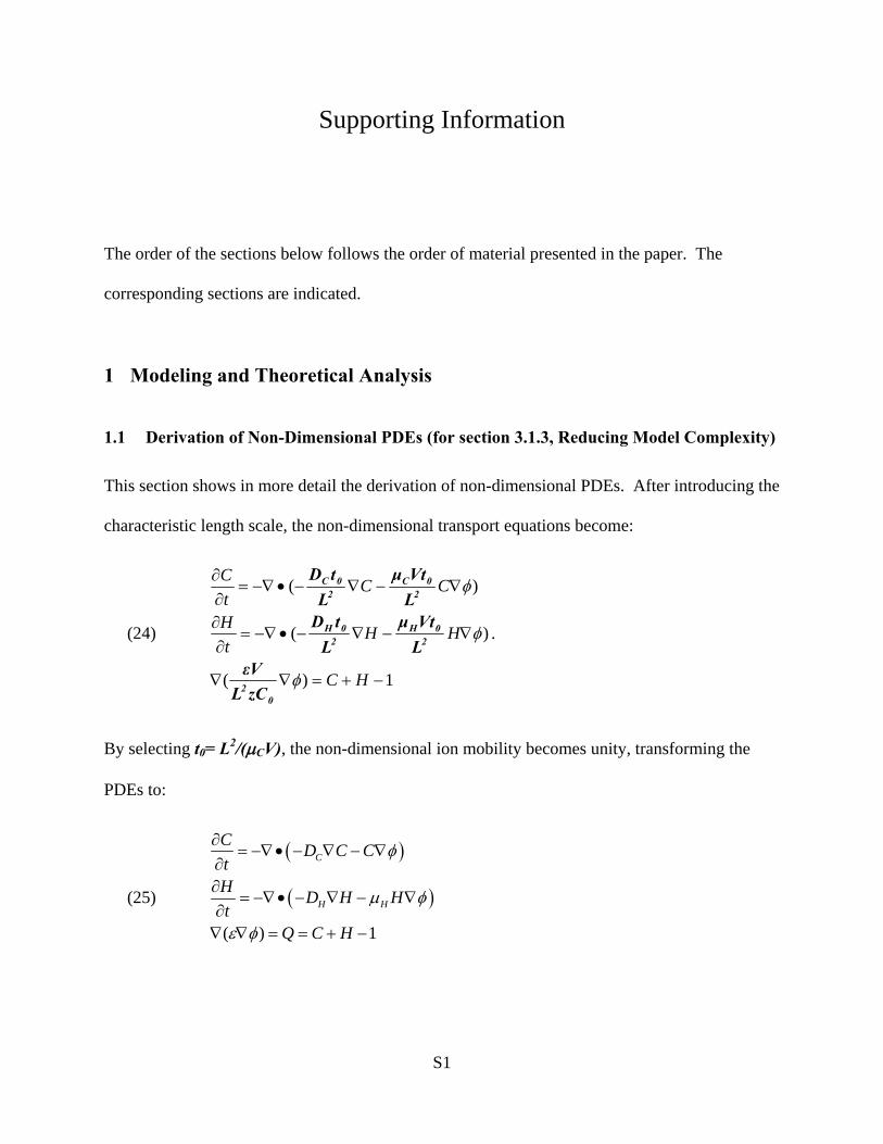
S1

Supporting Information

The order of the sections below follows the order of material presented in the paper. The

corresponding sections are indicated.

1 Modeling and Theoretical Analysis

1.1 Derivation of Non-Dimensional PDEs (for section 3.1.3, Reducing Model Complexity)

This section shows in more detail the derivation of non-dimensional PDEs. After introducing the

characteristic length scale, the non-dimensional transport equations become:

(24)

1)(

)(

)(

−+=∇∇

∇−∇−•−∇=∂

∂

∇−∇−•−∇=∂∂

HC

HHt

H

CCtC

φ

φ

φ

02

20H

20H

20C

20C

zCLεV

LVtμ

LtD

LVtμ

LtD

.

By selecting t0= L2/(μCV), the non-dimensional ion mobility becomes unity, transforming the

PDEs to:

(25)

( )

( )( ) 1

C

H H

C D C CtH D H Ht

Q C H

φ

μ φ

ε φ

∂= −∇ • − ∇ − ∇

∂∂

= −∇ • − ∇ − ∇∂

∇ ∇ = = + −

S2

CD is given by the ratio between dimensional diffusion DC and drift magnitude μCV,

/CD = C CD Vμ . CD has units of m2/s, Cμ has units of m2/Vs, and V has units of V. Hence, CD

is non-dimensional. The hole diffusion coefficient is scaled the same way, /HD = H CD Vμ . The

non-dimensional mobilities are 1Cμ = and /Hμ = H Cμ μ . Finally, the non-dimensional

dielectric coefficient /ε = 20 maxV L Hε is the dimensional coefficient ε normalized by the

characteristic gradient of the electric field ( )/ ~ / /0 0 0E L V L L divided by the maximum charge

concentration Hmax.

1.2 Derivation of Governing Equations with Enforced Charge Neutrality (for section

4.3.4, Charge Neutrality Strictly Enforced)

Consider the governing equations (9) in the main text. Adding together equations (9)a and (9) b

gives

(26) )]()[()( φμφμ ∇−∇−+∇−∇−•−∇=∂+∂ HHDCCDt

HCHHCC .

To enforce charge neutrality, we set ε = 0 in (9)c which forces net charge Q = C + H –1 = 0.

This sets the left hand side of (26) to zero since C + H = 1 is constant. So now

(27) 0 [( ) ( )] [( ) ( )] [( ) ( ) )]

C C H H

C C H H

C H C H

D C C D H HD C C D C HD D C C H

μ φ μ φμ φ μ φ

μ μ φ

= −∇ • − ∇ − ∇ + − ∇ − ∇= −∇ • − ∇ − ∇ + ∇ − ∇= −∇ • − + ∇ − + ∇

where we have used H = 1 – C to substitute H C∇ = −∇ (second line). By charge neutrality,

knowing C immediately provides H, and this eliminates the need for equation (9)b. Both

equation (9)a and (26) contain an ion diffusion term, and the two terms conflict. (This is because

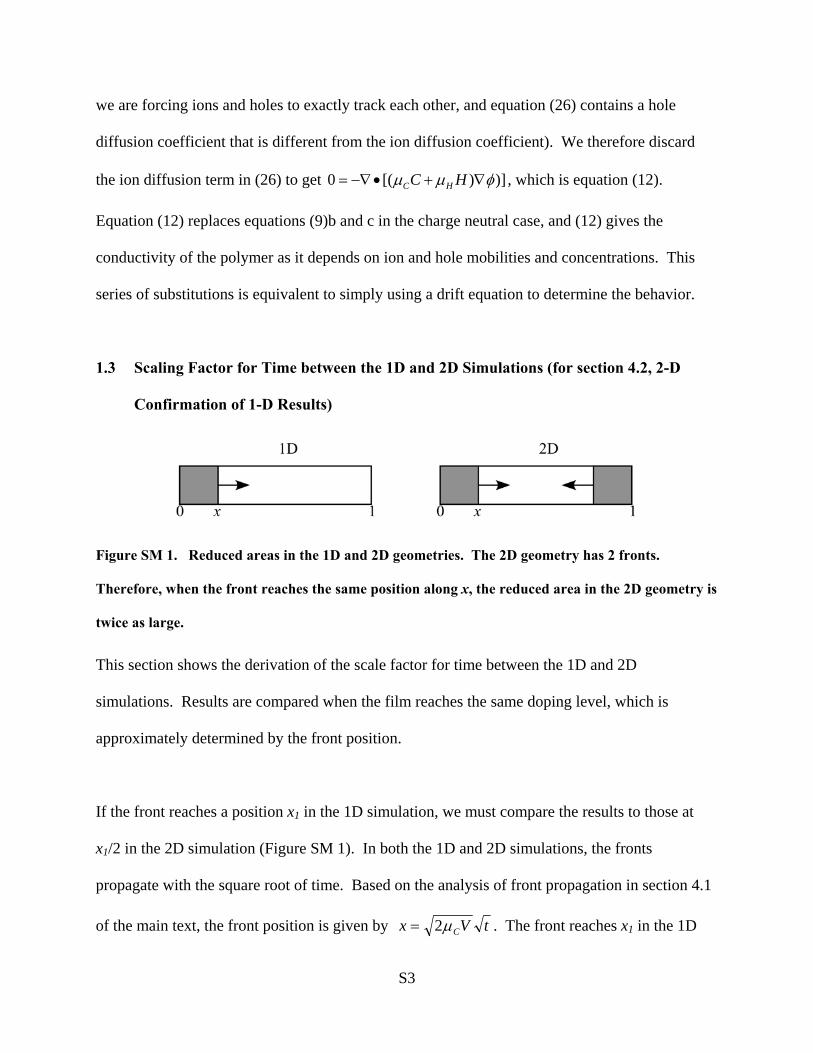
S3

we are forcing ions and holes to exactly track each other, and equation (26) contains a hole

diffusion coefficient that is different from the ion diffusion coefficient). We therefore discard

the ion diffusion term in (26) to get 0 [( ) )]C HC Hμ μ φ= −∇ • + ∇ , which is equation (12).

Equation (12) replaces equations (9)b and c in the charge neutral case, and (12) gives the

conductivity of the polymer as it depends on ion and hole mobilities and concentrations. This

series of substitutions is equivalent to simply using a drift equation to determine the behavior.

1.3 Scaling Factor for Time between the 1D and 2D Simulations (for section 4.2, 2-D

Confirmation of 1-D Results)

Figure SM 1. Reduced areas in the 1D and 2D geometries. The 2D geometry has 2 fronts.

Therefore, when the front reaches the same position along x, the reduced area in the 2D geometry is

twice as large.

This section shows the derivation of the scale factor for time between the 1D and 2D

simulations. Results are compared when the film reaches the same doping level, which is

approximately determined by the front position.

If the front reaches a position x1 in the 1D simulation, we must compare the results to those at

x1/2 in the 2D simulation (Figure SM 1). In both the 1D and 2D simulations, the fronts

propagate with the square root of time. Based on the analysis of front propagation in section 4.1

of the main text, the front position is given by tVx Cμ2= . The front reaches x1 in the 1D

S4

simulation at time t1 = (x1/ Vcμ2 )2. In the 2D simulation, the front reaches x1/2 at t2

=

[(x1/2) VCμ2 ]2. The ratio between t1 and t2 is thus t2 = t1/4. The scaling factor is unaffected by

the constants used in the non-dimensionalization.

2 Base Case Simulation

2.1 Variation of Dielectric Constant (for section Error! Reference source not found., Error!

Reference source not found.)

This section demonstrates that using a non-dimensional dielectric constant ε of 0.001, which is 8

orders of magnitude larger than the actual value (10-11~10-8), does not affect the front

propagation results during reduction. The actual value cannot be used in the simulation because

it is so much smaller than the other variables, which are close to 1: that would requires mesh

densities that cannot be handled, due to limitations in computer memory.

To demonstrate that ε reaches a limiting value, the simulation was run with 4 different dielectric

constants: 0.1, 0.01, 0.001, and 0.0001. The results converged, as shown in Figure SM 2, for ε <

0.001 (results for 0.001 and 0.0001 overlapped).

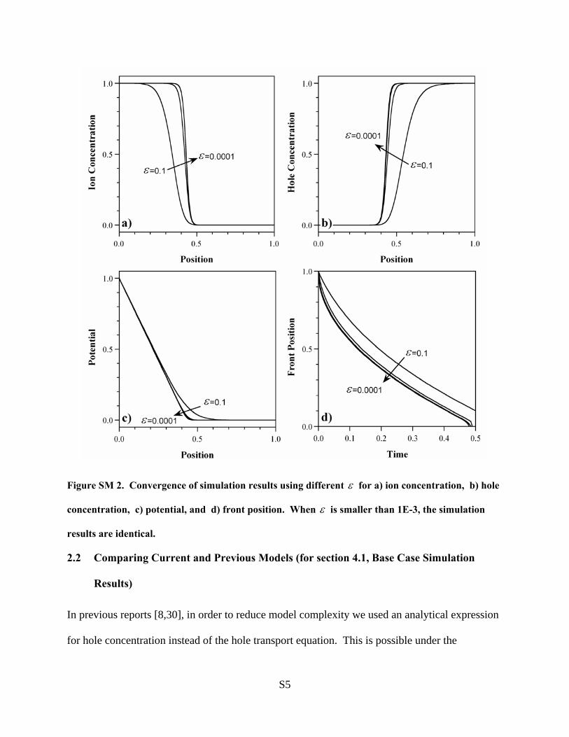
S5

Figure SM 2. Convergence of simulation results using different ε for a) ion concentration, b) hole

concentration, c) potential, and d) front position. When ε is smaller than 1E-3, the simulation

results are identical.

2.2 Comparing Current and Previous Models (for section 4.1, Base Case Simulation

Results)

In previous reports [8,30], in order to reduce model complexity we used an analytical expression

for hole concentration instead of the hole transport equation. This is possible under the

S6

assumption that hole transport occurs much faster than ion transport, since in that case the hole

concentration can be linked to the potential. Here we compare the ion concentrations in the base

case model with those in that prior model (Figure SM 3) and find that they are identical.

Figure SM 3. Comparison of the ion concentration profiles obtained by solving the three PDEs of

equation (9) (gray line) with those obtained using an analytical solution for the holes (points).

One might ask, what is advantage of the current model, if the results are identical? The 3rd PDE

allows us to study a wider range of cases: cases in which μH is not >> μC, in which non-constant

coefficients are used, and in which the model is used to predict oxidation.

S7

2.3 Net Charge and Front Broading at Different Reduction Potentials (for section 4.3.1,

Voltage)

Figure SM 4 shows the net charge in the film under higher (V = 1.5) and much lower (V = 0.001)

reduction potentials than in the base case (V = 1). At very low potential, the film is basically

charge-neutral everywhere. With increasing reduction potential, the net charge at the front

increases, and its distribution narrows.

Figure SM 4. Net charge in the polymer for different reduction potentials when the polymer is

approximately half-way reduced.

The effective broadening velocity was determined from the width of the front at time t = 0.1.

This is plotted in Figure SM 5 as a function of the applied potential. The broadening decreases

approximately as 1/√V.

S8

Figure SM 5. Effective front broadening velocity (width at t = 0.1) vs. potential. The curve is the

line y = 0.148*V-0.5.

2.4 Front Propagation along the Electric Field Line in the 2-D Base Case (for section 4.2,

2-D Confirmation of 1-D Results)

Figure SM 6 compares the front propagation along the electric field line in the 2D simulation

with front propagation in the 1D simulation. The front position for the 2D simulation was

obtained from the ion concentration profile along the electrical field streamline at y = 0.15. The

front moves slightly faster in the 2D case.

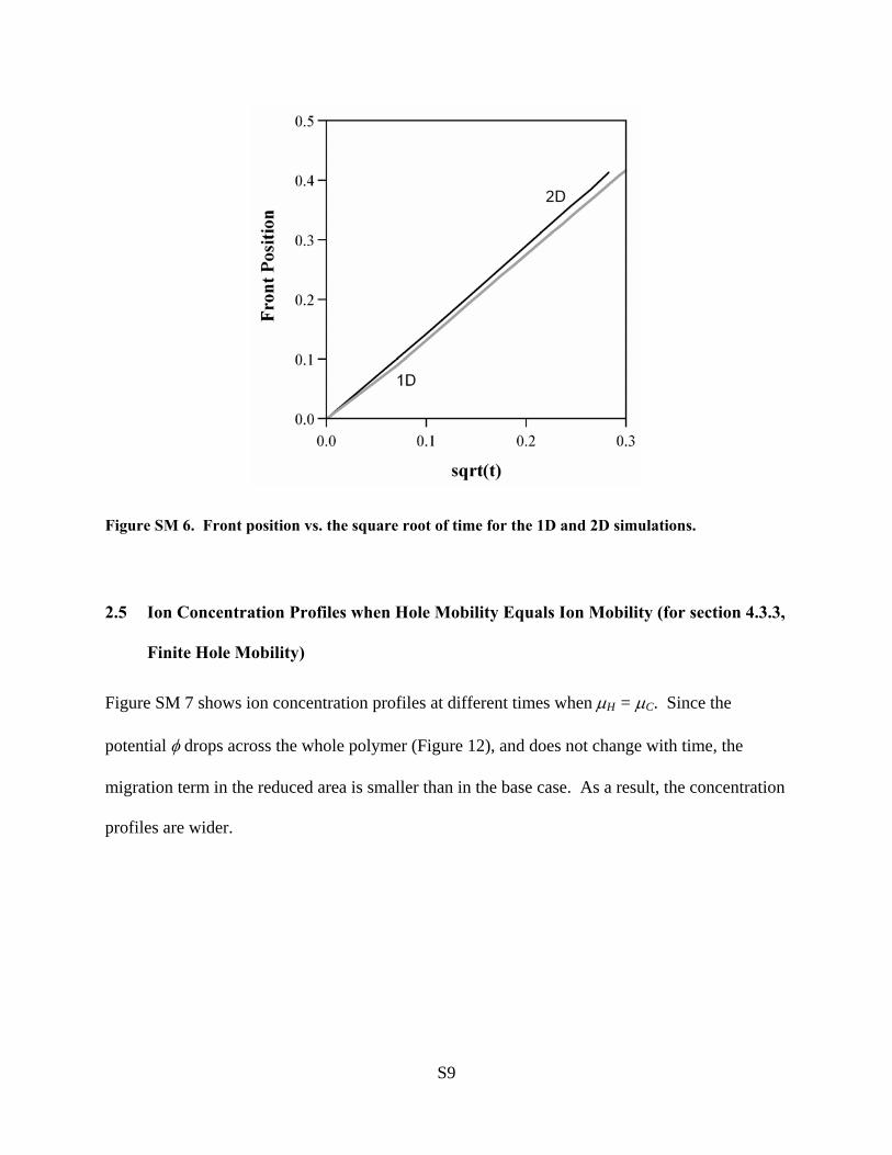
S9

Figure SM 6. Front position vs. the square root of time for the 1D and 2D simulations.

2.5 Ion Concentration Profiles when Hole Mobility Equals Ion Mobility (for section 4.3.3,

Finite Hole Mobility)

Figure SM 7 shows ion concentration profiles at different times when μH = μC. Since the

potential φ drops across the whole polymer (Figure 12), and does not change with time, the

migration term in the reduced area is smaller than in the base case. As a result, the concentration

profiles are wider.

S10

Figure SM 7. Ion concentration profiles when μH = μC at three times during reduction.

2.6 Effect of Concentration at the Polymer/Electrolyte Interface (for section 3.1.2.2,

Boundary and Initial Conditions)

Figure SM 8 and Figure SM 9 show how the ion concentration at the polymer/electrolyte

interface affects the simulation results. The lower concentration value represents the bulk

electrolyte concentration (0.03), and the higher value the concentration in the double layer (2.00).

The maximum ion concentration in the polymer (C =C0 = 1) used in the base case is shown for

comparison.

Within the bulk of the polymer, all three profiles have the same shape: the reduced area has C =

1, and the oxidized area has C = 0. However, using a lower concentration results in a slower-

S11

moving front (Figure SM 9). It also has this interesting effect: it makes the front move linearly

with time.

Figure SM 8. Ion concentration profiles for different ion concentrations at x = 0; the gray line

shows the base case, in which C|x=0 = 1.

S12

Figure SM 9. Front propagations when different values are used for different ion concentrations at

the polymer/electrolyte interface.

2.7 Base Case Simulation with Only Diffusion for Ions and Holes (for section 4.3.1,

Voltage)

Figure SM 10 shows ion and hole concentrations at different time snapshots when they are both

driven by diffusion only. In this simulation, the hole boundary condition at the electrode is set to

zero (rather than using the flux boundary condition, which causes the simulation to crash).

While the ion profiles resemble those in Figure 9c, the hole profiles bear no relation to what they

should because if ions and holes are driven by diffusion only, their movement becomes

uncoupled (charge neutrality cannot be enforced). As a result, this case leads to unphysical

results, as is also illustrated by the potential profile (Figure SM 11).

S13

Figure SM 10. a) Ion concentration profiles at t = 0.01, 0.2, and 1.0 for a simulation in which ions

and holes move by diffusion only. b) The corresponding hole concentrations. Since holes have

1000 times higher mobility, they leave the film quickly.

The ions diffuse into the polymer (Figure SM 10a) because at the electrolyte/polymer boundary,

C = 1. If this were set to another value, then these curves would simply be multiplied in height

accordingly, with the final equilibrium value in the polymer equal to the concentration set at the

boundary.

S14

Figure SM 11. Potential profiles at three times during a simulation in which ions and holes move

only by diffusion.

2.8 Base Case with Charge Neutrality Enforced (for section 4.3.4, Charge Neutrality

Strictly Enforced)

Ion concentration profiles at different times from the charge neutrality case are shown in Figure

SM 12a. As in the base case, the ions travel into the film at a front, and this front broadens over

time. In addition (not shown), once again the speed of the front was proportional to V.

The potential profile at t = 0.25 is presented in Figure SM 12b. Although the potential drops

mainly in the reduced area, since the hole mobility was only 5 times higher than that of the ions,

a portion of the potential also drops in the oxidized area. If it were possible to use a higher hole

mobility in the simulation, the results would have resembled the base case more closely.

S15

Figure SM 12. a) Ion concentration profiles at different times when charge neutrality is enforced in

the polymer. Note that the hole mobility is only 5 times that of ions (necessary for the simulation to

run). b) Potential profiles at t = 0.25 for the charge neutral (black line) and base (gray line) cases.

The front position vs. time with charge neutrality strictly enforced is shown in Figure SM 13.

Again because μH/μC = 5, this front moves more slowly (there is a smaller voltage drop across

the reduced region) and the velocity is more constant. These results arise from the small hole

mobility, not from enforcing charge neutrality.

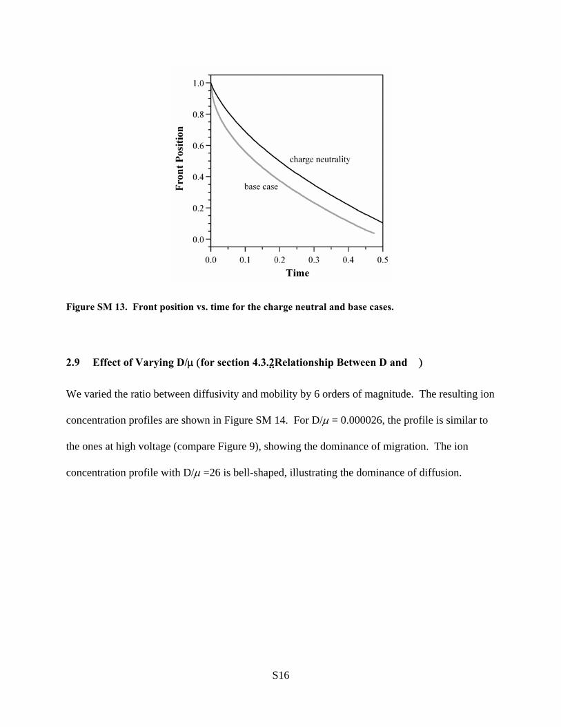
S16

Figure SM 13. Front position vs. time for the charge neutral and base cases.

2.9 Effect of Varying D/μ (for section 4.3.2Relationship Between D and �)

We varied the ratio between diffusivity and mobility by 6 orders of magnitude. The resulting ion

concentration profiles are shown in Figure SM 14. For D/μ = 0.000026, the profile is similar to

the ones at high voltage (compare Figure 9), showing the dominance of migration. The ion

concentration profile with D/μ =26 is bell-shaped, illustrating the dominance of diffusion.

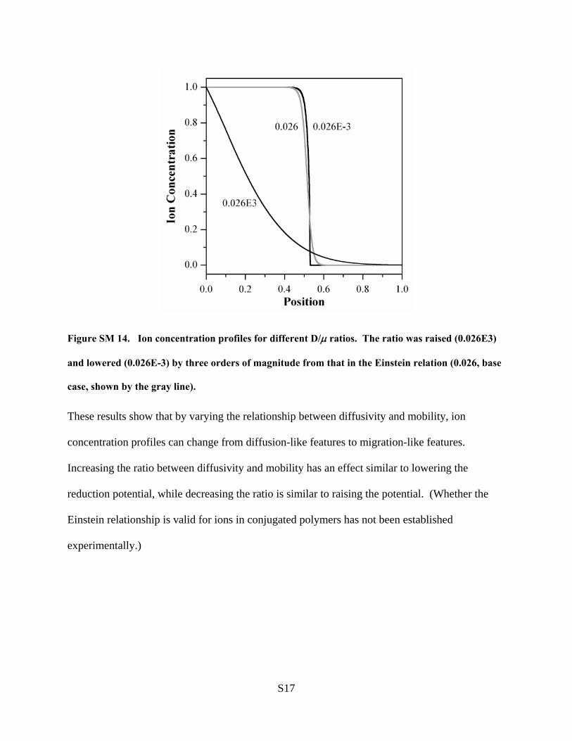
S17

Figure SM 14. Ion concentration profiles for different D/μ ratios. The ratio was raised (0.026E3)

and lowered (0.026E-3) by three orders of magnitude from that in the Einstein relation (0.026, base

case, shown by the gray line).

These results show that by varying the relationship between diffusivity and mobility, ion

concentration profiles can change from diffusion-like features to migration-like features.

Increasing the ratio between diffusivity and mobility has an effect similar to lowering the

reduction potential, while decreasing the ratio is similar to raising the potential. (Whether the

Einstein relationship is valid for ions in conjugated polymers has not been established

experimentally.)

S18

3 Reduction in the Full Model

3.1 Ion Flux in the Electrolyte (for section 5.2, Addition of the Electrolyte)

The section compares the drift and diffusion terms in the electrolyte to determine the importance

of drift in the electrolyte. As shown in Figure SM 15a, the ions in the electrolyte move

exclusively by drift between x = -10 and -5, and increasingly by diffusion closer to the polymer

interface, where there are substantial concentration gradients. Then, within 0.03 distance units of

the polymer interface (Figure SM 15b), the migration component increases again, to large

positive values, and the diffusion component goes to large negative values: the strong electric

field pulls the cations toward the interface, but at the same time the high concentration of cations

in the double-layer produces a large flux away from the interface back into the electrolyte.

These two components approximately balance, the difference being the flux into the polymer.

Figure SM 15. a) Diffusive and drift fluxes of cations in the electrolyte far from the polymer. B)

Diffusive and drift fluxes in the double layer. Note the differences in scale from a).

S19

3.2 Potential Drop over the Polymer (for section 5.2.2, Full Model Results)

Figure SM 16 shows the potential drop across the polymer over time in the full model, which

includes the electrolyte. It increases rapidly until t = 0.01 and then grows slowly until the film is

fully reduced at t = 0.2.

Figure SM 16. Potential drop over the polymer film over time in the full model (V = -1); the rest of

the voltage is dropped over the electrolyte.

3.3 Comparison between Full Model and Base Case (for section 5.2.2, Full Model Results)

Figure SM 17 shows the ion concentration profiles predicted by the models in sections 5.1 and

5.2 at the same time (t = 0.08) when V = 0.25 is applied in the former, and V = 1 in the latter.

The only difference is that the base case profile is slightly ahead of that in the full model. This is

because the ion concentration at the polymer/electrolyte interface in the full model is smaller

S20

than Cmax (= 1). The two models thus behave the same way when the potentials across the

polymer are the same.

Figure SM 17. Results at t = 0.08 from the full model with an applied potential of V = 1.0 (black)

and the base case model with an applied potential of V = 0.25 (gray). a) Ion concentration, b) hole

concentration, c) potential, and d) front position.

S21

3.4 Full Model with Diffusion Only (for section 5.2.3, Variation: Diffusion Only)

In the paper, we showed the result of neglecting cation migration in the polymer. Here we

present four additional simulations in which the full model is driven by diffusion only. In the

first, we examine how the addition of a capping function changes the results presented in the

main text. In the second, the cation mobility in the polymer is set to zero and the diffusivity is

given a stronger dependence on ion concentration. In the third, both ions and holes in the

polymer are driven by diffusion only. In the last case, the ions in the electrolyte are driven by

diffusion only.

3.4.1 Diffusion-Based Capping Function

The case presented in the paper could not employ a migration-based capping function for the

charge, since the migration term was already set to zero everywhere. This section instead uses a

capping function based on diffusion:

(28) DC = D0 (1+ 0.01e15(C - 0.8)).

Figure SM 18 compares the ion concentration profiles for diffusion-only in the polymer with

(black) and without (gray) capping. The only difference is that in the latter case, the profiles are

slightly more advanced, but the effect is small because the ion concentration in the film never

goes that high. For example, at t = 0.02, the ion concentration at the interface is only 1.15,

resulting in a diffusivity increase of 2.9 there.

S22

Figure SM 18. Ion concentration profiles (black lines) when migration in the polymer is turned off

and the capping function in equation (28) is applied. The gray lines show the profiles without

capping.

3.4.2 Ion Diffusivity Proportional to e5C

This section examines how the simulation results are affected when a steeper relationship

between diffusivity and ion concentration is used: e2C is replaced by e5C. At low potentials (< 1),

the maximum ion concentration was always lower than 1 (Figure SM 19a), even after long times.

At high potentials (Figure SM 19b), C reached Cmax, although it exceeded Cmax at early times.

The final ion concentration is shown as a function of voltage in Figure SM 19c. When the

reduction voltage is increased, the front velocity increases logarithmically (Figure SM 19d),

which is inconsistent with the experimental results. The front velocity increases because higher

voltages lead to higher ion concentrations at the interface.

S23

Figure SM 19. Ion concentrations and front velocities during reduction when ion migration is

turned off in the polymer and DC = D0 e5C. Concentration profiles for a) V = 0.5 and b) V = 7. c)

Final ion concentrations in the polymer at the end of the reduction process for different applied

potentials. d) Front velocity vs. potential. The line shows a log fit.

3.4.3 Ions and Holes in the Polymer Driven by Diffusion Only

In the previous cases, the holes in the polymer were still moving by migration. Figure SM 20

shows the potentials in the polymer at two different times when migration is set to zero for both

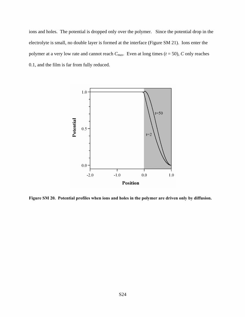
S24

ions and holes. The potential is dropped only over the polymer. Since the potential drop in the

electrolyte is small, no double layer is formed at the interface (Figure SM 21). Ions enter the

polymer at a very low rate and cannot reach Cmax. Even at long times (t = 50), C only reaches

0.1, and the film is far from fully reduced.

Figure SM 20. Potential profiles when ions and holes in the polymer are driven only by diffusion.

S25

Figure SM 21. Ion and hole concentrations when ions and holes in the polymer are driven only by

diffusion.

3.4.4 Ions in the Electrolyte Driven by Diffusion Only

This section examines the effect of turning off migration in the electrolyte (preventing the

transport of ions by migration to the electrolyte/polymer boundary), but leaving migration on in

the polymer. Figure SM 22 shows that under these conditions, the ion concentration in the

polymer remains equal to the bulk electrolyte concentration no matter how long the simulation

runs, and the film cannot be reduced.

S26

Figure SM 22. Ion and hole concentrations when ions in the electrolyte are driven only by

diffusion.

Article · its complexity is gradually increased to realize a full model that treats non-Fickian...

Documents

Transcript of Article · its complexity is gradually increased to realize a full model that treats non-Fickian...