Interactions Lectures 1 & 2 - York UniversityObservations 50)
22
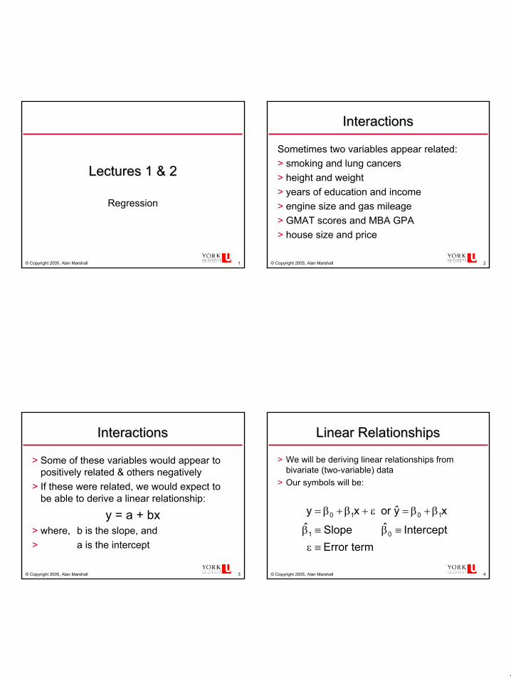
1 © Copyright 2005, Alan Marshall 1 Lectures 1 & 2 Lectures 1 & 2 Regression © Copyright 2005, Alan Marshall 2 Interactions Interactions Sometimes two variables appear related: > smoking and lung cancers > height and weight > years of education and income > engine size and gas mileage > GMAT scores and MBA GPA > house size and price © Copyright 2005, Alan Marshall 3 Interactions Interactions > Some of these variables would appear to positively related & others negatively > If these were related, we would expect to be able to derive a linear relationship: y = a + bx > where, b is the slope, and > a is the intercept © Copyright 2005, Alan Marshall 4 Linear Relationships Linear Relationships > We will be deriving linear relationships from bivariate (two-variable) data > Our symbols will be: term Error Intercept ˆ Slope ˆ x y ˆ or x y 0 1 1 0 1 0 ≡ ε ≡ β ≡ β β + β = ε + β + β =
Transcript of Interactions Lectures 1 & 2 - York UniversityObservations 50)
111
© Copyright 2005, Alan Marshall 1
Lectures 1 & 2Lectures 1 & 2
Regression
© Copyright 2005, Alan Marshall 2
InteractionsInteractions
Sometimes two variables appear related:> smoking and lung cancers> height and weight> years of education and income> engine size and gas mileage> GMAT scores and MBA GPA> house size and price
© Copyright 2005, Alan Marshall 3
InteractionsInteractions
> Some of these variables would appear to positively related & others negatively
> If these were related, we would expect to be able to derive a linear relationship:
y = a + bx> where, b is the slope, and> a is the intercept
© Copyright 2005, Alan Marshall 4
Linear RelationshipsLinear Relationships
> We will be deriving linear relationships from bivariate (two-variable) data
> Our symbols will be:
termErrorInterceptˆ Slopeˆ
xy or xy
01
1010
≡ε
≡β≡β
β+β=ε+β+β=

222
© Copyright 2005, Alan Marshall 5
Estimating a LineEstimating a Line
> The symbols for the estimated linear relationship are:
> b1 is our estimate of the slope, β1
> b0 is our estimate of the intercept, β0
xbby 10 +=
© Copyright 2005, Alan Marshall 6
ExampleExample
> Consider the following example comparing the returns of Consolidated Moose Pasture stock (CMP) and the TSX 300 Index
> The next slide shows 25 monthly returns
© Copyright 2005, Alan Marshall 7
Example DataExample Data
TSX CMP TSX CMP TSX CMPx y x y x y
3 4 -4 -3 2 4-1 -2 -1 0 -1 12 -2 0 -2 4 34 2 1 0 -2 -15 3 0 0 1 2
-3 -5 -3 1 -3 -4-5 -2 -3 -2 2 11 2 1 3 -2 -22 -1
© Copyright 2005, Alan Marshall 8
ExampleExample
> From the data, it appears that a positive relationship may exist• Most of the time when the TSX is up, CMP is
up• Likewise, when the TSX is down, CMP is down
most of the time• Sometimes, they move in opposite directions
> Let’s graph this data

333
© Copyright 2005, Alan Marshall 9
Graph Of DataGraph Of Data
-6
-4
-2
0
2
4
6
-6 -4 -2 0 2 4 6TSX
CMP
© Copyright 2005, Alan Marshall 10
Graph Of DataGraph Of Data
-6
-4
-2
0
2
4
6
-6 -4 -2 0 2 4 6TSE
CMP
© Copyright 2005, Alan Marshall 11
Example Summary StatisticsExample Summary Statistics
> The data do appear to be positively related> Let’s derive some summary statistics about these
data:
Mean s2 s TSX 0.00 7.25 2.69 CMP 0.00 6.25 2.50
© Copyright 2005, Alan Marshall 12
ObservationsObservations
> Both have means of zero and standard deviations just under 3
> However, each data point does not have simply one deviation from the mean, it deviates from both means
> Consider Points A, B, C and D on the next graph
444
© Copyright 2005, Alan Marshall 13
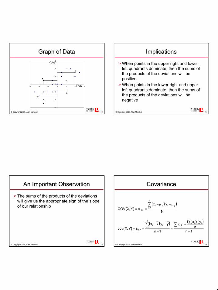
Graph of DataGraph of Data
-6
-4
-2
0
2
4
6
-6 -4 -2 0 2 4 6TSX
CMP
A
B
C
D
© Copyright 2005, Alan Marshall 14
ImplicationsImplications
> When points in the upper right and lower left quadrants dominate, then the sums of the products of the deviations will be positive
> When points in the lower right and upper left quadrants dominate, then the sums of the products of the deviations will be negative
© Copyright 2005, Alan Marshall 15
An Important ObservationAn Important Observation
> The sums of the products of the deviations will give us the appropriate sign of the slope of our relationship
© Copyright 2005, Alan Marshall 16
CovarianceCovariance
( )( )
( )( ) ( )
1nn
yxyx
1n
yyxxsYXcov
N
yxYXCOV
iiiii
n
1ii
XY
yi
N
1ixi
XY
−
−=
−
−−==
µ−µ−=σ≡
∑ ∑ ∑∑
∑
=
=
),(
),(

555
© Copyright 2005, Alan Marshall 17
CovarianceCovariance
-6
-4
-2
0
2
4
6
-6 -4 -2 0 2 4 6TSX
CMP
A
B
C
D
© Copyright 2005, Alan Marshall 18
CovarianceCovariance
> In the same units as Variance (if both variables are in the same unit), i.e. units squared
> Very important element of measuring portfolio risk in finance
© Copyright 2005, Alan Marshall 19
Using CovarianceUsing Covariance
> Very useful in Finance for measuring portfolio risk
> Unfortunately, it is hard to interpret for two reasons:• What does the magnitude/size imply?• The units are confusing
© Copyright 2005, Alan Marshall 20
A More Useful StatisticA More Useful Statistic
> We can simultaneously adjust for both of these shortcomings by dividing the covariance by the two relevant standard deviations
> This operation• Removes the impact of size & scale• Eliminates the units
666
© Copyright 2005, Alan Marshall 21
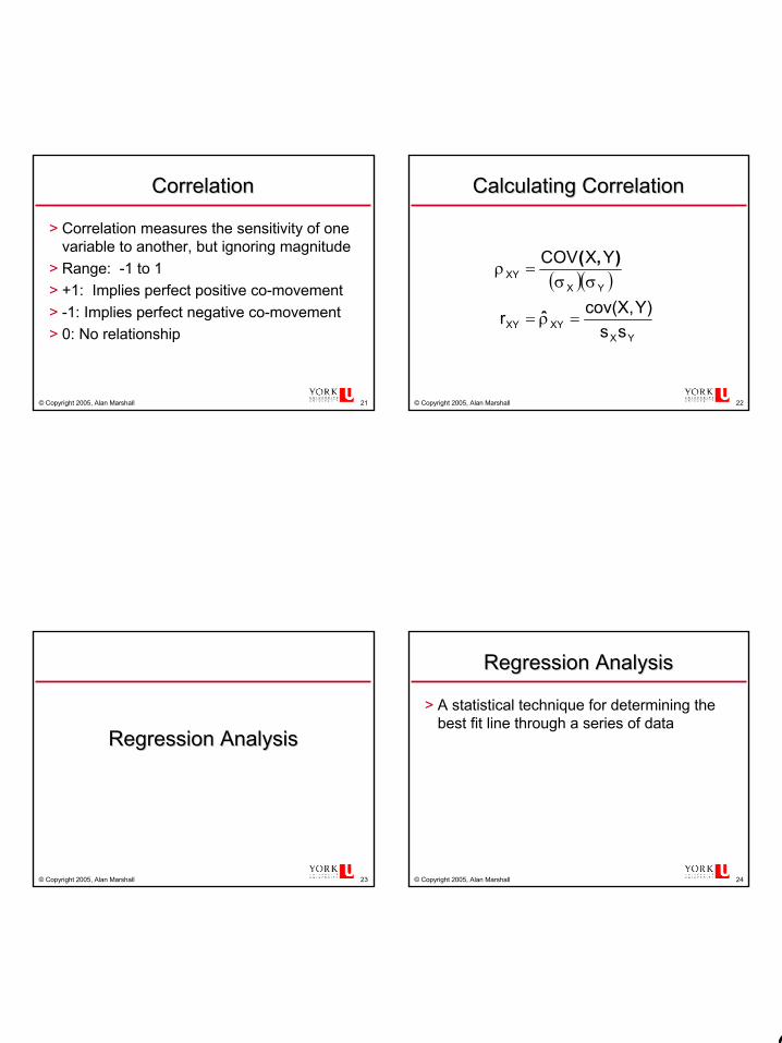
CorrelationCorrelation
> Correlation measures the sensitivity of one variable to another, but ignoring magnitude
> Range: -1 to 1> +1: Implies perfect positive co-movement> -1: Implies perfect negative co-movement> 0: No relationship
© Copyright 2005, Alan Marshall 22
Calculating CorrelationCalculating Correlation
( )( )
YXXYXY
YXXY
ssY)cov(X,r
YXCOV
=ρ=
σσ=ρ
ˆ
),(
© Copyright 2005, Alan Marshall 23
Regression AnalysisRegression Analysis
© Copyright 2005, Alan Marshall 24
Regression AnalysisRegression Analysis
> A statistical technique for determining the best fit line through a series of data

777
© Copyright 2005, Alan Marshall 25
ErrorError
> No line can hit all, or even most of the points -The amount we miss by is called ERROR
> Error does not mean mistake! It simply means the inevitable “missing” that will happen when we generalize, or try to describe things with models
> When we looked at the mean and variance, we called the errors deviations
© Copyright 2005, Alan Marshall 26
What Regression DoesWhat Regression Does
> Regression finds the line that minimizes the amount of error, or deviation from the line
> The mean is the statistic that has the minimum total of squared deviations
> Likewise, the regression line is the unique line that minimizes the total of the squared errors.
> The Statistical term is “Sum of Squared Errors” or SSE
© Copyright 2005, Alan Marshall 27
ExampleExample
> Suppose we are examining the sale prices of compact cars sold by rental agencies and that we have the following summary statistics:
© Copyright 2005, Alan Marshall 28
Summary StatisticsSummary StatisticsPrice
Mean 5411.41Median 5362Mode 5286Standard Deviation 254.9488004Range 1124Minimum 4787Maximum 5911Sum 541141Count 100
> Our best estimate of the average price would be $5,411
> Our 95% Confidence Interval would be $5,411 ± (2)(255) or $5,411 ± (510) or $4,901 to $5,921

888
© Copyright 2005, Alan Marshall 29
Something Missing?Something Missing?
> Clearly, looking at this data in such a simplistic way ignores a key factor: the mileage of the vehicle
© Copyright 2005, Alan Marshall 30
Price vs. MileagePrice vs. Mileage
0
1000
2000
3000
4000
5000
6000
7000
0 10000 20000 30000 40000 50000 60000
Odometer Reading
Pric
e
© Copyright 2005, Alan Marshall 31
Importance of the FactorImportance of the Factor
> After looking at the scatter graph, you would be inclined to revise you estimate depending on the mileage• 25,000 km about $5,700 - $5,900• 45,000 km about $5,100 - $5,300
> Similar to getting new information when we look at Bayes Theorem.
© Copyright 2005, Alan Marshall 32
Switch to ExcelSwitch to Excel
File CarPrice.xlsTab Odometer
999
© Copyright 2005, Alan Marshall 33
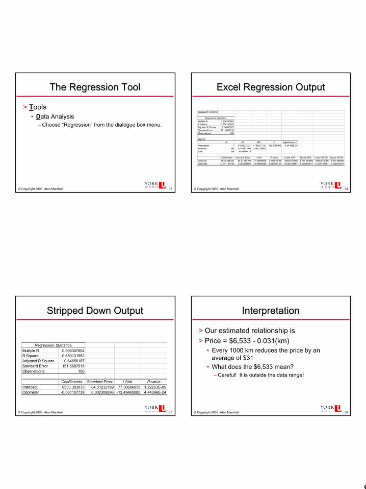
The Regression ToolThe Regression Tool
> Tools• Data Analysis
– Choose “Regression” from the dialogue box menu.
© Copyright 2005, Alan Marshall 34
Excel Regression OutputExcel Regression Output
SUMMARY OUTPUT
Regression StatisticsMultiple R 0.806307604R Square 0.650131952Adjusted R Square 0.64656187Standard Error 151.5687515Observations 100
ANOVAdf SS MS F Significance F
Regression 1 4183527.721 4183527.721 182.1056015 4.44346E-24Residual 98 2251362.469 22973.08642Total 99 6434890.19
Coefficients Standard Error t Stat P-value Lower 95% Upper 95% Lower 95.0% Upper 95.0%Intercept 6533.383035 84.51232199 77.30686935 1.22253E-89 6365.671086 6701.094984 6365.671086 6701.094984Odometer -0.031157739 0.002308896 -13.49465085 4.44346E-24 -0.035739667 -0.026575811 -0.035739667 -0.026575811
© Copyright 2005, Alan Marshall 35
Stripped Down OutputStripped Down Output
Regression StatisticsMultiple R 0.806307604R Square 0.650131952Adjusted R Square 0.64656187Standard Error 151.5687515Observations 100
Coefficients Standard Error t Stat P-valueIntercept 6533.383035 84.51232199 77.30686935 1.22253E-89Odometer -0.031157739 0.002308896 -13.49465085 4.44346E-24
© Copyright 2005, Alan Marshall 36
InterpretationInterpretation
> Our estimated relationship is> Price = $6,533 - 0.031(km)
• Every 1000 km reduces the price by an average of $31
• What does the $6,533 mean?– Careful! It is outside the data range!
101010
© Copyright 2005, Alan Marshall 37
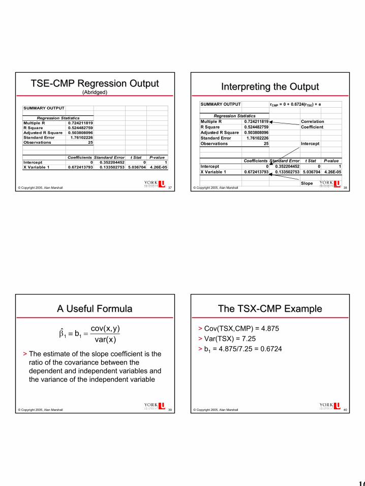
TSETSE--CMP Regression OutputCMP Regression Output(Abridged)(Abridged)
SUMMARY OUTPUT
Regression StatisticsMultiple R 0.724211819R Square 0.524482759Adjusted R Square 0.503808096Standard Error 1.76102226Observations 25
Coefficients Standard Error t Stat P-valueIntercept 0 0.352204452 0 1X Variable 1 0.672413793 0.133502753 5.036704 4.26E-05
© Copyright 2005, Alan Marshall 38
Interpreting the OutputInterpreting the OutputSUMMARY OUTPUT rCMP = 0 + 0.6724(rTSE) + e
Regression StatisticsMultiple R 0.724211819 CorrelationR Square 0.524482759 CoefficientAdjusted R Square 0.503808096Standard Error 1.76102226Observations 25 Intercept
Coefficients Standard Error t Stat P-valueIntercept 0 0.352204452 0 1X Variable 1 0.672413793 0.133502753 5.036704 4.26E-05
Slope
© Copyright 2005, Alan Marshall 39
A Useful FormulaA Useful Formula
> The estimate of the slope coefficient is the ratio of the covariance between the dependent and independent variables and the variance of the independent variable
)xvar()y,xcov(bˆ
11 =≡β
© Copyright 2005, Alan Marshall 40
The TSXThe TSX--CMP ExampleCMP Example
> Cov(TSX,CMP) = 4.875> Var(TSX) = 7.25> b1 = 4.875/7.25 = 0.6724

111111
© Copyright 2005, Alan Marshall 41
Required Conditions Required Conditions -- εε
> The probability distribution of ε is normal> E(ε) = 0> σε is constant and independent of x, the
independent variable> The value of ε associated with any
particular value of y is independent of the value of ε associated with any other value of y
© Copyright 2005, Alan Marshall 42
Assessing the ModelAssessing the Model
© Copyright 2005, Alan Marshall 43
SSE & SEESSE & SEE
> SSE: Sum of Squares for Error• This is the sum of the squared errors from the
regression line> SEE: Standard Error of Estimate
2nSSEs−
=ε
© Copyright 2005, Alan Marshall 44
SSE & SEESSE & SEE
> We want these to be as small as possible> Our best test is the F-ratio from the ANOVA
table• To see if the SSE is small relative to the SSR,
Sum of Squares for the Regression> In Excel, the “Error” is called the residual

121212
© Copyright 2005, Alan Marshall 45
F RatioF Ratio
> From the Car Price example:
> The F ratio is very large, and the p-value is minute, so we can conclude that the model has some significance
ANOVAdf SS MS F Significance F
Regression 1 4183527.72 4183527.72 182.1056 4.44346E-24Residual 98 2251362.47 22973.0864Total 99 6434890.19
© Copyright 2005, Alan Marshall 46
Testing the SlopeTesting the Slope
> The regression output tells us the standard deviation of the slope coefficient estimate
> We are most often interested in testing to see if the estimated slope is non-zero
HO: β1 = 0> Sometimes test whether the slope is some
other value, i.e., HO: β1 = 1
© Copyright 2005, Alan Marshall 47
Testing the SlopeTesting the Slope
> From the Car Price Example
> The t-ratio is very large and the p-value very small, so there is strong evidence that the slope is non-zero
Coefficients Standard Error t Stat P-valueIntercept 6533.383035 84.51232199 77.30687 1.2225E-89Odometer -0.031157739 0.002308896 -13.4947 4.4435E-24
© Copyright 2005, Alan Marshall 48
TSXTSX--CMP ExampleCMP ExampleSUMMARY OUTPUT rCMP = 0 + 0.6724(rTSE) + e
Regression StatisticsMultiple R 0.724211819 CorrelationR Square 0.524482759 CoefficientAdjusted R Square 0.503808096Standard Error 1.76102226Observations 25 Intercept
Coefficients Standard Error t Stat P-valueIntercept 0 0.352204452 0 1X Variable 1 0.672413793 0.133502753 5.036704 4.26E-05
Slope

131313
© Copyright 2005, Alan Marshall 49
TSXTSX--CMP ExampleCMP Example
> We can easily see that the test of the slope indicates that it is non-zero
> Is the slope different from 1?HO: β1 = 1
© Copyright 2005, Alan Marshall 50
TSXTSX--CMP ExampleCMP Example
064.2t454.21335.03276.0
1335.016724.0
sbt
24,025.0
11
1
=>=
=−
=
β−=
β
We reject the null hypothesis, HO: β1 = 1. There is evidence that the slope is less than 1
© Copyright 2005, Alan Marshall 51
RR22: Coefficient of Determination: Coefficient of Determination
> The R2 (“R-squared”) tells of the proportion of the variability in our dependent variable is explained by the independent variable
> It is the square of the correlation coefficient> It can also be computed from the ANOVA
table
© Copyright 2005, Alan Marshall 52
Car Price ExampleCar Price ExampleRegression Statistics
Multiple R 0.80631R Square 0.65013Adjusted R Square 0.64656Standard Error 151.569Observations 100
ANOVAdf SS MS F
Regression 1 4183527.7 4183528 182.106Residual 98 2251362.5 22973.09Total 99 6434890.2

141414
© Copyright 2005, Alan Marshall 53
Car Price Example: QualityCar Price Example: Quality
> Logical: Price is lowered as mileage increases, and by a plausible amount.
> The slope: 13.5σ from 0!• Occurs randomly, or by chance, with a
probability that has 23 zeros!> The R-squared: 0.65: 65% of the variation
in price is explained by mileage> F Ratio is high
© Copyright 2005, Alan Marshall 54
Symmetry in TestingSymmetry in TestingSUMMARY OUTPUT
Regression StatisticsMultiple R 0.806307604R Square 0.650131952Adjusted R Square 0.64656187Standard Error 151.5687515Observations 100
ANOVAdf SS MS F Significance F
Regression 1 4183527.721 4183527.721 182.1056015 4.44346E-24Residual 98 2251362.469 22973.08642Total 99 6434890.19
Coefficients Standard Error t Stat P-valueIntercept 6533.383035 84.51232199 77.30686935 1.22253E-89Odometer -0.031157739 0.002308896 -13.49465085 4.44346E-24
© Copyright 2005, Alan Marshall 55
The Correlation CoefficientThe Correlation Coefficient
> We can test the significance of the correlation coefficient
2r
2
r
r12nr
srt
2nr1s
−−
==
−−
=
© Copyright 2005, Alan Marshall 56
In the Car Price ExampleIn the Car Price Example
( )( )
( )
( )( )49.13
736.168063.034988.0988063.0
8063.0121008063.0t 2
−=−=
−=
−−−
−=

151515
© Copyright 2005, Alan Marshall 57
More ConsistencyMore Consistency
> Notice that this is the same t value that we had for the test of the slope
© Copyright 2005, Alan Marshall 58
Predicting Values with the Predicting Values with the Regression EquationRegression Equation
© Copyright 2005, Alan Marshall 59
PredictionPrediction
> Suppose you wanted to know what price you would get for a car, of the same model as those tested in our example with 40,000 km.
y = 6533.4 - 0.03116(40,000) = 5,287> Once again, we have the situation of a
point estimate, when we are likely most interested in a range or interval.
© Copyright 2005, Alan Marshall 60
Prediction IntervalsPrediction Intervals
( )( ) 2
x
2g
2n,2/ s1nxx
n11sty
−−
++± ε−α

161616
© Copyright 2005, Alan Marshall 61
In Our ExampleIn Our Example
( )( ) ( )( )( )
( )
5,589.76 to 4,984.2476.302287,5
3104,309,340,15,924,48901.1712.300287,5
690,528,439945.009,36000,40
1001157.151984.1287,5
2
±
+±
−++±
© Copyright 2005, Alan Marshall 62
Different ProblemDifferent Problem
> Suppose I am managing a fleet and decide to sell these cars once they have reached 40,000 km. What is the expected price I will get for the cars following this policy?
> Instead of predicting an individual value, I am asking for an expected value
> Similar to a CI of the mean vs. the CI of an individual value
© Copyright 2005, Alan Marshall 63
Expected Value Expected Value -- Interval EstimateInterval Estimate
( )( ) 2
x
2g
2n,2/ s1nxx
n1sty
−−
+± ε−α
© Copyright 2005, Alan Marshall 64
EV EV -- Interval EstimateInterval Estimate
( )( ) 2
x
2g
2n,2/ s1nxx
n1sty
−−
+± ε−α
Just like the confidence intervals
we saw in ADMS3320
Adjustment for the distance from the mean of the data

171717
© Copyright 2005, Alan Marshall 65
In Our ExampleIn Our Example
( )( ) ( )( )( )
( )
( )( )
5,322.19 to 5,251.8119.35287,5
.0.117027..712.300287,53104,309,340,
15,924,48901.0712.300287,5
690,528,439945.009,36000,40
100157.151984.1287,5
2
±±
+±
−+±
© Copyright 2005, Alan Marshall 66
Prediction Prediction vsvs Interval EstimateInterval Estimate
> Prediction Interval for a single observation of the dependent variable at a given value of the independent variable:
4,984.24 to 5,589.79> Interval Estimate for a mean value of the
dependent variable at a given value of the independent variable:
5,251.81 to 5,322.19
© Copyright 2005, Alan Marshall 67
Prediction Prediction vsvs Interval EstimateInterval Estimate
4,500
5,500
6,500
18,000 23,000 28,000 33,000 38,000 43,000 48,000
Odometer
Pric
e
Prediction Interval
Interval Estimate
© Copyright 2005, Alan Marshall 68
Multiple RegressionMultiple Regression
Using More than One Explanatory Variable
181818
© Copyright 2005, Alan Marshall 69
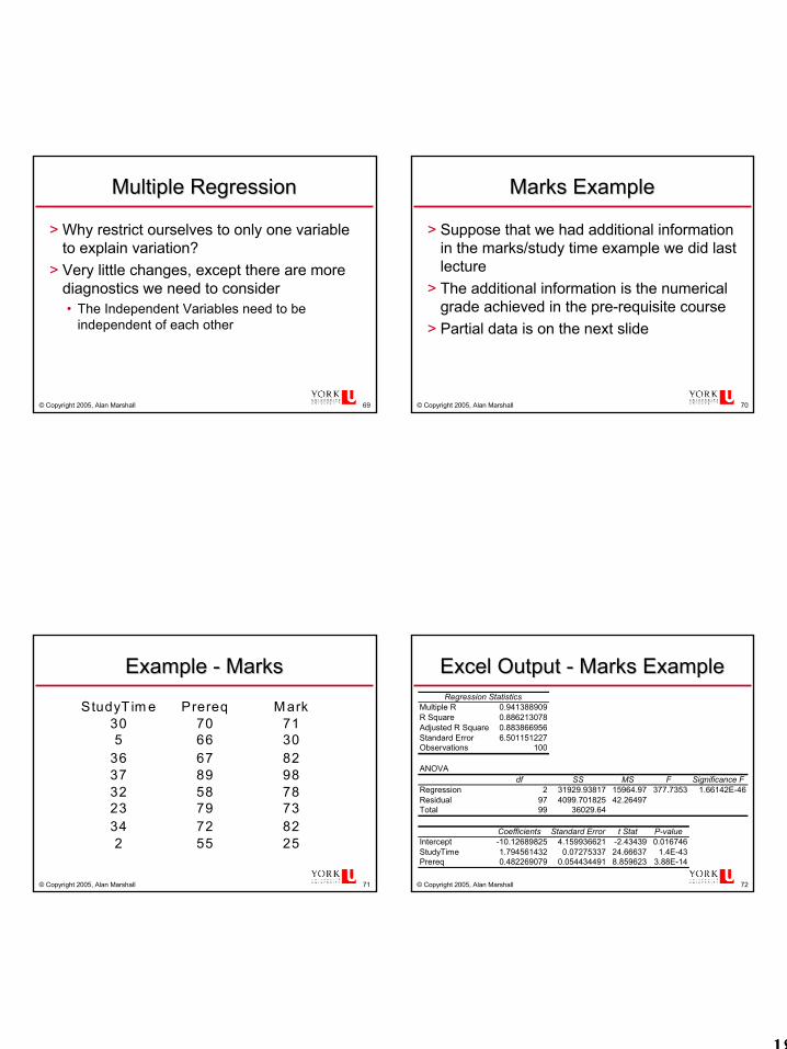
Multiple RegressionMultiple Regression
> Why restrict ourselves to only one variable to explain variation?
> Very little changes, except there are more diagnostics we need to consider• The Independent Variables need to be
independent of each other
© Copyright 2005, Alan Marshall 70
Marks ExampleMarks Example
> Suppose that we had additional information in the marks/study time example we did last lecture
> The additional information is the numerical grade achieved in the pre-requisite course
> Partial data is on the next slide
© Copyright 2005, Alan Marshall 71
Example Example -- MarksMarks
StudyT im e Prereq Mark30 70 715 66 30
36 67 8237 89 9832 58 7823 79 7334 72 822 55 25
© Copyright 2005, Alan Marshall 72
Excel Output Excel Output -- Marks ExampleMarks ExampleRegression Statistics
Multiple R 0.941388909R Square 0.886213078Adjusted R Square 0.883866956Standard Error 6.501151227Observations 100
ANOVAdf SS MS F Significance F
Regression 2 31929.93817 15964.97 377.7353 1.66142E-46Residual 97 4099.701825 42.26497Total 99 36029.64
Coefficients Standard Error t Stat P-valueIntercept -10.12689825 4.159936621 -2.43439 0.016746StudyTime 1.794561432 0.07275337 24.66637 1.4E-43Prereq 0.482269079 0.054434491 8.859623 3.88E-14
191919
© Copyright 2005, Alan Marshall 73
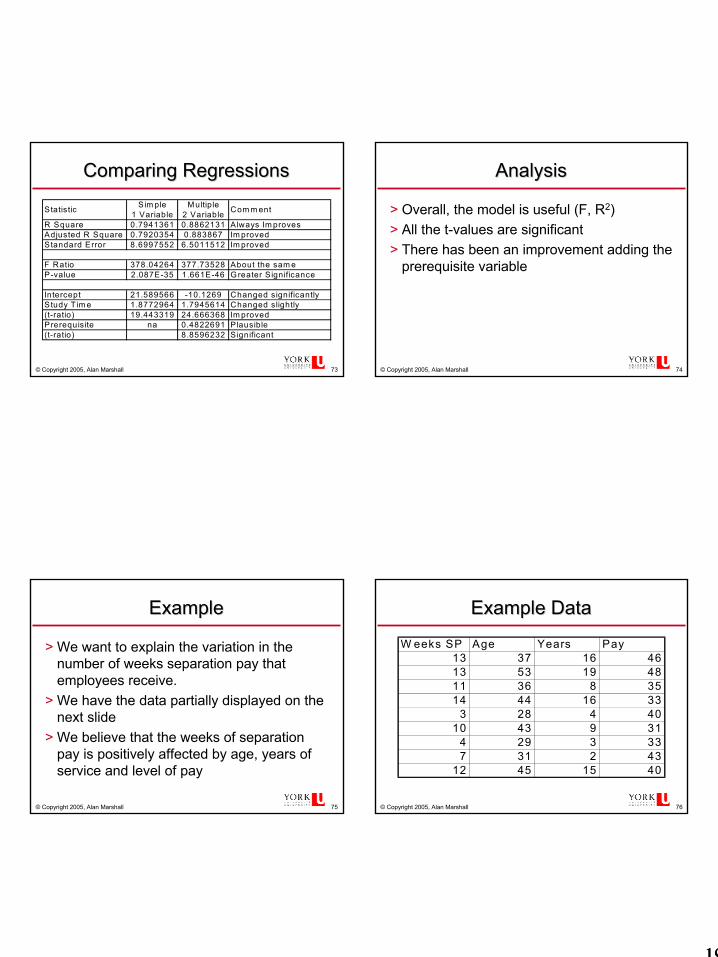
Comparing RegressionsComparing RegressionsSim ple Multiple
1 Variable 2 VariableR Square 0.7941361 0.8862131 Always Im provesAdjusted R Square 0.7920354 0.883867 Im provedStandard Error 8.6997552 6.5011512 Im proved
F Ratio 378.04264 377.73528 About the sam eP-value 2.087E-35 1.661E-46 G reater Significance
Intercept 21.589566 -10.1269 Changed significantlyStudy T im e 1.8772964 1.7945614 Changed slightly(t-ratio) 19.443319 24.666368 Im provedPrerequisite na 0.4822691 Plausible(t-ratio) 8.8596232 Significant
Com m entStatistic
© Copyright 2005, Alan Marshall 74
AnalysisAnalysis
> Overall, the model is useful (F, R2)> All the t-values are significant> There has been an improvement adding the
prerequisite variable
© Copyright 2005, Alan Marshall 75
ExampleExample
> We want to explain the variation in the number of weeks separation pay that employees receive.
> We have the data partially displayed on the next slide
> We believe that the weeks of separation pay is positively affected by age, years of service and level of pay
© Copyright 2005, Alan Marshall 76
Example DataExample Data
W eeks SP Age Years Pay13 37 16 4613 53 19 4811 36 8 3514 44 16 33
3 28 4 4010 43 9 31
4 29 3 337 31 2 43
12 45 15 40

202020
© Copyright 2005, Alan Marshall 77
Excel OutputExcel OutputRegression Statistics
Multiple R 0.837841R Square 0.701977Adjusted R Square 0.682541Standard Error 1.921049Observations 50
ANOVAdf SS MS F Signif. F
Regression 3 399.8602 133.2867 36.11686 3.7583E-12Residual 46 169.7598 3.69043Total 49 569.62
Coeff. Std Error t Stat P-valueIntercept 6.061146 2.604023 2.327608 0.024387Age -0.00781 0.066414 -0.11754 0.906946Years 0.603482 0.09656 6.249804 1.22E-07Pay -0.07025 0.05237 -1.34133 0.186399
© Copyright 2005, Alan Marshall 78
AnalysisAnalysis
> Overall, the model is useful (F, R2)> The “Years” variable is significant
• “Age” and “Pay” are not• We should consider dropping these variables• Age and Years are probably correlated
© Copyright 2005, Alan Marshall 79
CorrelationsCorrelations
Weeks SP Age Years PayWeeks SP 1Age 0.670007 1Years 0.830853 0.807963 1Pay 0.112985 0.17253 0.260971 1
> Indeed, Age and Years are highly correlated> Let’s drop Age, with the highest correlation with
the years and the lowest t-value, and see if the model improves
© Copyright 2005, Alan Marshall 80
Dropping AgeDropping AgeRegression StatisticsMultiple R 0.837787R Square 0.701888Adjusted R 0.689202Standard E 1.900788Observatio 50
ANOVAdf SS MS F Signif. F
Regression 2 399.8093 199.9046 55.32935 4.45E-13Residual 47 169.8107 3.612995Total 49 569.62
Coeff. Std Error t Stat P-valueIntercept 5.840082 1.781987 3.277286 0.001975Years 0.594376 0.057024 10.42334 8.26E-14Pay -0.06983 0.0517 -1.35069 0.183262

212121
© Copyright 2005, Alan Marshall 81
AnalysisAnalysis
> The F ratio has improved (55 vs. 36)• The t ratio for Years has also improved
> The t ratio for Pay has not improved> Let’s drop Pay
© Copyright 2005, Alan Marshall 82
Simple ModelSimple ModelRegression Statistics
Multiple R 0.830853R Square 0.690316Adjusted R Square 0.683864Standard Error 1.917041Observations 50
ANOVAdf SS MS F Signif. F
Regression 1 393.2178 393.2178 106.9967 8.27E-14Residual 48 176.4022 3.675045Total 49 569.62
Coeff. Std Error t Stat P-valueIntercept 3.621377 0.696703 5.197878 4.1E-06Years 0.574275 0.055518 10.34392 8.27E-14
© Copyright 2005, Alan Marshall 83
AnalysisAnalysis
> This model is an improvement• F-ratio increased a lot (107 vs. 55)
> Years is the only variable significant in explaining the number of weeks of severance pay
© Copyright 2005, Alan Marshall 84
To Watch ForTo Watch For
> Variables significantly related to each other• Correlation Function (Tools Data Analysis)• Look for values above 0.5 or below -0.5
> Nonsensical Results• Wrong Signs
> Weak Variables• Magnitude of the T-ratio less than 2• p-value greater than 0.05

222222
© Copyright 2005, Alan Marshall 85
YOU LEARN STATISTICSYOU LEARN STATISTICSBY DOING STATISTICSBY DOING STATISTICS