![[XLS]faculty.chicagobooth.edufaculty.chicagobooth.edu/news/Cases_Jan09-Oct12.xlsx · Web view9/11/2009 9/10/2012 9/11/2009 3/9/2012 3/20/2009 12/23/2009 3/20/2009 5/1/2009 8/7/2009](https://static.fdocuments.net/doc/165x107/5ae501d37f8b9a90138fc3d9/xls-view9112009-9102012-9112009-392012-3202009-12232009-3202009.jpg)
faculty.chicagobooth.edufaculty.chicagobooth.edu/midwest.econometrics/Papers/MEGWu.pdf ·...
61
Identication and Estimation of Gaussian A¢ ne Term Structure Models James D. Hamilton y Department of Economics University of California, San Diego Jing (Cynthia) Wu z Department of Economics University of California, San Diego June 18, 2010 Revised: December 11, 2010 Abstract This paper develops new results for both identication and estimation of Gaussian a¢ ne term structure models. In terms of identication, we establish that three pop- ular canonical representations are each, for di/erent reasons, unidentied. We also demonstrate that a failure of local identication can complicate numerical search for the maximum-likelihood estimate when one uses conventional estimation methods. A sep- arate contribution of the paper is the proposal of minimum-chi-square estimation as an alternative to maximum-likelihood estimation. We show that, although it is asymptoti- cally equivalent or sometimes even identical to MLE, it can be much easier to compute. In some cases, MCSE allows the researcher to recognize with certainty whether a given estimate represents a global maximum of the likelihood function and makes feasible the computation of small-sample standard errors. We are grateful to Bryan Brown, Michael Bauer and Ken Singleton for comments on an earlier draft. y [email protected] z [email protected] 1
Transcript of faculty.chicagobooth.edufaculty.chicagobooth.edu/midwest.econometrics/Papers/MEGWu.pdf ·...
Identi�cation and Estimation of Gaussian A¢ ne Term
Structure Models�
James D. Hamiltony
Department of Economics
University of California, San Diego
Jing (Cynthia) Wuz
Department of Economics
University of California, San Diego
June 18, 2010Revised: December 11, 2010
Abstract
This paper develops new results for both identi�cation and estimation of Gaussian
a¢ ne term structure models. In terms of identi�cation, we establish that three pop-
ular canonical representations are each, for di¤erent reasons, unidenti�ed. We also
demonstrate that a failure of local identi�cation can complicate numerical search for the
maximum-likelihood estimate when one uses conventional estimation methods. A sep-
arate contribution of the paper is the proposal of minimum-chi-square estimation as an
alternative to maximum-likelihood estimation. We show that, although it is asymptoti-
cally equivalent or sometimes even identical to MLE, it can be much easier to compute.
In some cases, MCSE allows the researcher to recognize with certainty whether a given
estimate represents a global maximum of the likelihood function and makes feasible the
computation of small-sample standard errors.
�We are grateful to Bryan Brown, Michael Bauer and Ken Singleton for comments on an earlier [email protected]@ucsd.edu
1

1 Introduction.
The class of Gaussian a¢ ne term structure models1 developed by Vasicek (1977), Du¢ e and
Kan (1996), Dai and Singleton (2002), and Du¤ee (2002) has become the basic workhorse in
macroeconomics and �nance for purposes of using a no-arbitrage framework for studying the
relations between yields on assets of di¤erent maturities. Its appeal comes from its simple
characterization of how risk gets priced by the market which, under the assumption of no
arbitrage, generates predictions for the price of any asset. The approach has been used to
measure the role of risk premia in interest rates (Du¤ee, 2002; Cochrane and Piazzesi, 2009),
study how macroeconomic developments and monetary policy a¤ect the term structure of
interest rates (Ang and Piazzesi, 2003; Beechey and Wright, 2009; Bauer, 2009), characterize
the monetary policy rule (Ang, Dong and Piazzesi, 2007; Rudebusch and Wu, 2008; Bekaert,
Cho and Moreno, 2010), determine why long-term yields remained remarkably low in 2004 and
2005 (Kim andWright, 2005; Rudebusch, Swanson andWu, 2006), infer market expectations of
in�ation from the spread between nominal and in�ation-indexed Treasury yields (Christensen,
Lopez and Rudebusch, 2010), evaluate the e¤ectiveness of the extraordinary central bank
interventions during the �nancial crisis (Christensen, Lopez and Rudebusch, 2009; Smith,
2010), and study the potential for monetary policy to a¤ect interest rates when the short rate
is at the zero lower bound Hamilton and Wu (2010a).
But buried in the footnotes of this literature and in the practical experience of those
who have used these models are tremendous numerical challenges in estimating the necessary
1By Gaussian a¢ ne term structure models we refer to speci�cations in which the discrete-time joint dis-tribution of yields and factors is multivariate Normal with constant conditional variances. We do not in thispaper consider the broader class of non-Gaussian processes.
2

parameters from the data due to highly non-linear and badly-behaved likelihood surfaces. For
example, Kim (2008) observed:
Flexibly speci�ed no-arbitrage models tend to entail much estimation di¢ culty
due to a large number of parameters to be estimated and due to the nonlinear
relationship between the parameters and yields that necessitates a nonlinear opti-
mization.
Ang and Piazzesi (2003) similarly reported:
di¢ culties associated with estimating a model with many factors using maxi-
mum likelihood when yields are highly persistent....We need to �nd good starting
values to achieve convergence in this highly non-linear system....[T]he likelihood
surface is very �at in �0 which determines the mean of long yields....
This paper proposes a solution to these and other problems with a¢ ne term structure
models based on what we will refer to as their reduced-form representation. For a popular
class of Gaussian a¢ ne term structure models�namely, those for which the model is claimed
to price exactly a subset of N` linear combinations of observed yields, where N` is the number
of unobserved pricing factors�this reduced form is a restricted vector autoregression in the
observed set of yields and macroeconomic variables. More generally, the reduced form is
a restricted state-space representation for the set of observed variables. We explore two
implications of this fact that seem to have been ignored in the large preceding literature on
such models.
3

The �rst is that the parameters of these reduced-form representations contain all the
observable implications of any Gaussian a¢ ne term structure model for the sample of observed
data. Hence, as noted by Fisher (1966) and Rothenberg (1971), we can use the reduced-form
representation to characterize the identi�ability of any parameters that might be of interest.
If more than one value for the parameter vector of interest is associated with the same reduced-
form parameter vector, then the model is unidenti�ed at that point and there is no way to
use the observed data to distinguish between the alternative possibilities. We show using this
approach that three popular parameterizations of a¢ ne term structure models�namely, the
preferred representations proposed by Dai and Singleton (2000), Ang and Piazzesi (2003) and
Pericoli and Taboga (2008)�are in fact unidenti�ed. While the lack of identi�cation of the
Dai and Singleton (2000) representation has previously been established by Collin-Dufresne,
Goldstein and Jones (2008) and Aït-Sahalia and Kimmel (2010) using other methods, the
results for the Ang and Piazzesi (2003) and Pericoli and Taboga (2008) approaches are new.
We further demonstrate that it is common for numerical search methods to end up in regions
of the parameter space that are locally unidenti�ed, and show why this failure of identi�cation
arises. These issues of identi�cation are one factor that contributes to the numerical di¢ culties
for conventional methods noted above.
A second and completely separate contribution of the paper is the observation that it is
possible for the parameters of interest to be inferred directly from estimates of the reduced-
form parameters themselves. This is a very useful result because the latter are often simple
OLS coe¢ cients. Although translating from reduced-form parameters into structural para-
meters involves a mix of analytical and numerical calculations, the numerical component is
4

far simpler than that associated with the usual approach of trying to �nd the maximum of the
likelihood surface directly as a function of the structural parameters. In the case of a just-
identi�ed structure, the numerical component of our proposed method has an additional big
advantage over the traditional approach, in that the researcher knows with certainty whether
the equations have been solved, and therefore knows with certainty whether one has found the
global maximum of the likelihood surface with respect to the structural parameters or simply
a local maximum. In the conventional approach, one instead has to search over hundreds of
di¤erent starting values, and even then has no guarantee that the global maximum has been
found. In the case where the model imposes overidentifying restrictions on the reduced form,
one can still estimate structural parameters as functions of the unrestricted reduced-form
estimates by the method of minimum-chi-square estimation described by Rothenberg (1973,
pp. 24-25).2 This minimizes a quadratic form in the di¤erence between the reduced-form pa-
rameters implied by a given structural model and the reduced-form parameters as estimated
without restrictions directly from the data, with weights coming from the information matrix.
Among other illustrations of the computational bene�ts of this approach, we establish the
feasibility of calculating small-sample standard errors and con�dence intervals for this class of
models and demonstrate that the parameter estimates reported by Ang and Piazzesi (2003)
in fact correspond to a local maximum of the likelihood surface and are not the global MLE.
There have been several other recent e¤orts to address many of these problems. Chris-
tensen, Diebold and Rudebusch (forthcoming) develop a no-arbitrage representation of a dy-
namic Nelson-Siegel model of interest rates that gives a convenient representation of level,
2Minimum-chi-square estimation has also been used in other settings by Chamberlain (1982) and Newey(1987).
5
slope and curvature factors and o¤ers signi�cant improvements in empirical tractability and
predictive performance over earlier a¢ ne term structure speci�cations. Joslin, Singleton and
Zhu (forthcoming) propose a canonical representation for a¢ ne term structure models that
greatly improves convergence of maximum likelihood estimation. Collin-Dufresne, Goldstein
and Jones (2008) propose a representation in terms of the derivatives of the term structure
at maturity zero, arguing for the bene�ts of using these observable magnitudes rather than
unobserved latent variables to represent the state vector of an ATSM. Each of these pa-
pers proposes canonical representations that are identi�ed, and the Christensen, Diebold and
Rudebusch (forthcoming) and Joslin, Singleton and Zhu (forthcoming) parameterizations lead
to better behaved likelihood functions than do the parameterizations explored in detail in our
paper.
The chief di¤erence between our proposed solution and those of these other researchers
is that they focus on how the ATSM should be represented, whereas we examine how the
parameters of the ATSM are to be estimated. Thus for example Christensen, Diebold and
Rudebusch (forthcoming) require the researcher to impose certain restrictions on the ATSM,
whereas Joslin, Singleton and Zhu (forthcoming) cannot incorporate most auxiliary restric-
tions on the P dynamics. It is far from clear how any of these three approaches could have
been used to estimate a model of the form investigated by Ang and Piazzesi (2003). By con-
trast, our minimum-chi-square algorithm can be used for any representation, including those
proposed by Christensen, Diebold and Rudebusch (forthcoming) and Joslin, Singleton and
Zhu (forthcoming), and can simplify the numerical burden regardless of the representation
chosen. Indeed, some of the numerical advantages of Joslin, Singleton and Zhu (forthcom-
6

ing) come from the fact that a subset of their parameterization is identical to a subset of our
reduced-form representation, and their approach, like ours, takes advantage of the fact that
the full-information MLE for this subset can be obtained by OLS for a popular class of mod-
els. However, Joslin, Singleton and Zhu (forthcoming) estimate the remaining parameters by
conventional MLE rather than using the full set of reduced-form estimates as in our approach.
As Joslin, Singleton and Zhu (forthcoming) note, their representation becomes unidenti�ed in
the presence of a unit root. When applied to highly persistent data, we illustrate that their
MLE algorithm can encounter similar problems to those of other representations, which can
be avoided with our approach to parameter estimation.
Our estimation strategy is related to that of Bekaert, Cho andMoreno (2010), who estimate
structural parameters to match the moments of the reduced-form representation using the
generalized method of moments (GMM). Whereas our approach uses OLS estimation to
simplify greatly the numerical estimation problem, their approach requires all parameters to
be estimated together from scratch in a single GMM problem that retains all of the numerical
challenges associated with MLE.
The rest of the paper is organized as follows. Section 2 describes the class of Gaussian a¢ ne
term structure models and three popular examples, and brie�y uses one of the speci�cations
to illustrate the numerical di¢ culties that can be encountered with the traditional approach.
Section 3 investigates the mapping from structural to reduced-form parameters. We establish
that the canonical forms of all three examples are unidenti�ed and explore how this contributes
to some of the problems for conventional numerical search algorithms. In Section 4 we use
the mapping to propose approaches to parameter estimation that are much better behaved.
7

Section 5 concludes.
2 Gaussian A¢ ne Term Structure Models.
2.1 Basic framework
Consider an (M � 1) vector of variables Ft whose dynamics are characterized by a Gaussian
vector autoregression:
Ft+1 = c+ �Ft + �ut+1 (1)
with ut � i.i.d. N(0; IM): This speci�cation implies that Ft+1jFt; Ft�1; :::; F1 � N(�t;��0)
for
�t = c+ �Ft: (2)
Let rt denote the risk-free one-period interest rate. If the vector Ft includes all the variables
that could matter to investors, then the price of a pure discount asset at date t should be a
function Pt(Ft) of the current state vector. Moreover, if investors were risk neutral, the price
they�d be willing to pay would satisfy
Pt(Ft) = exp(�rt)Et [Pt+1(Ft+1)]
= exp(�rt)ZRM
Pt+1(Ft+1)�(Ft+1;�t;��0) dFt+1 (3)
8
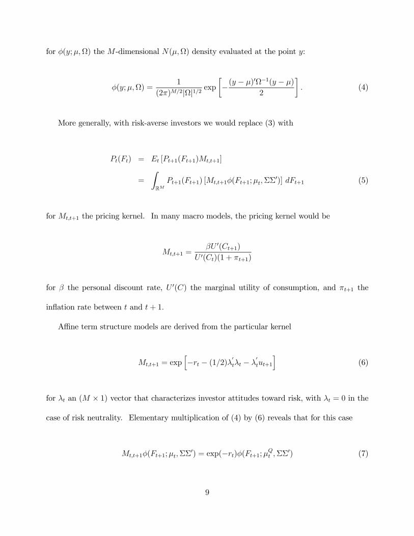
for �(y;�;) the M -dimensional N(�;) density evaluated at the point y:
�(y;�;) =1
(2�)M=2jj1=2 exp��(y � �)0�1(y � �)
2
�: (4)
More generally, with risk-averse investors we would replace (3) with
Pt(Ft) = Et [Pt+1(Ft+1)Mt;t+1]
=
ZRM
Pt+1(Ft+1) [Mt;t+1�(Ft+1;�t;��0)] dFt+1 (5)
for Mt;t+1 the pricing kernel. In many macro models, the pricing kernel would be
Mt;t+1 =�U 0(Ct+1)
U 0(Ct)(1 + �t+1)
for � the personal discount rate, U 0(C) the marginal utility of consumption, and �t+1 the
in�ation rate between t and t+ 1:
A¢ ne term structure models are derived from the particular kernel
Mt;t+1 = exph�rt � (1=2)�
0
t�t � �0
tut+1
i(6)
for �t an (M � 1) vector that characterizes investor attitudes toward risk, with �t = 0 in the
case of risk neutrality. Elementary multiplication of (4) by (6) reveals that for this case
Mt;t+1�(Ft+1;�t;��0) = exp(�rt)�(Ft+1;�Qt ;��0) (7)
9

for
�Qt = �t � ��t: (8)
Substituting (7) into (5) and comparing with (3), we see that for this speci�cation of the
pricing kernel, risk-averse investors value any asset the same as risk-neutral investors would if
the latter thought that the conditional mean of Ft+1 was �Qt rather than �t. A positive value
for the �rst element of �t, for example, implies that an asset that delivers the quantity F1;t+1
dollars in period t + 1 would have a value at time t that is less than the value that would
be assigned by a risk-neutral investor, and the size of this di¤erence is bigger when the (1; 1)
element of � is bigger. An asset yielding Fi;t+1 dollars has a market value that is reduced
by �i1�1t relative to a risk-neutral valuation, through the covariance between factors i and 1.
The term �1t might then be described as the market price of factor 1 risk.
The a¢ ne term structure models further postulate that this market price of risk is itself
an a¢ ne function of Ft;
�t = �+ �Ft (9)
for � an (M � 1) vector and � an (M �M) matrix. Substituting (9) and (2) into (8), we see
that
�Qt = cQ + �QFt
for
cQ = c� �� (10)
�Q = �� ��: (11)
10

In other words, risk-averse investors value assets the same way as a risk-neutral investor would
if that risk-neutral investor believed that the factors are characterized by a Q-measure VAR
given by
Ft+1 = cQ + �QFt + �uQt+1 (12)
with uQt+1 a vector of independent standard Normal variables under the Q measure.
Suppose that the risk-free 1-period yield is also an a¢ ne function of the factors
rt = �0 + �0
1Ft: (13)
Then, as demonstrated for example in Appendix A of Ang and Piazzesi (2003), under the
above assumptions the yield on a risk-free n-period pure-discount bond can be calculated as
ynt = an + b0nFt (14)
where
bn =1
n
hIM + �Q0 + � � �+
��Q0�n�1i
�1 (15)
an = �0 +�b01 + 2b
02 + � � �+ (n� 1) b0n�1
�cQ=n (16)
��b01��
0b1 + 22b02��
0b2 + � � �+ (n� 1)2 b0n�1��0bn�1�=2n:
If we knew Ft and the values of cQ and �Q along with �0; �1; and �, we could use (14), (15),
and (16) to predict the yield for any maturity n.
There are thus three sets of parameters that go into an a¢ ne term structure model: (a)
11

the parameters c; �; and � that characterize the objective dynamics of the factors in equation
(1) (sometimes called the P parameters); (b) the parameters � and � in equation (9) that
characterize the price of risk; and (c) the Q parameters cQ and �Q (along with the same �
as appeared in the P parameter set) that �gure in (12). If we knew any two of these sets of
parameters, we could calculate the third3 using (10) and (11). We will refer to a representation
in terms of (a) and (b) as a � representation, and a representation in terms of (a) and (c) as
a Q representation.
Suppose we want to describe yields on a set of Nd di¤erent maturities: If Nd is greater
than N`, where N` is the number of unobserved pricing factors, then (14) would imply that
it should be possible to predict the value of one of the ynt as an exact linear function of
the others. Although in practice we can predict one yield extremely accurately given the
others, the empirical �t is never exact. One common approach to estimation, employed for
example by Ang and Piazzesi (2003) and Chen and Scott (1993), is to suppose that (14) holds
exactly for N` linear combinations of observed yields, and that the remaining Ne = Nd � N`
linear combinations di¤er from the predicted value by a small measurement error. Let Y 1t
denote the (N`� 1) vector consisting of those linear combinations of yields that are treated as
priced without error and Y 2t the remaining (Ne � 1) linear combinations. The measurement
3We will discuss examples below in which � is singular for which the demonstration of this equivalence isa bit more involved, with the truth of the assertion coming from the fact that for such cases certain elementsof � and � are de�ned to be zero.
12

speci�cation is then
26664Y 1t
(N`�1)
Y 2t
(Ne�1)
37775 =26664
A1(N`�1)
A2(Ne�1)
37775+26664
B1(N`�M)
B2(Ne�M)
37775Ft +26664
0(N`�Ne)
�e(Ne�Ne)
37775 uet(Ne�1)
(17)
where �e is typically taken to be diagonal. Here Ai and Bi are calculated by stacking (16) and
(15), respectively, for the appropriate n, while �e determines the variance of the measurement
error with uet � N(0; INe): We will discuss many of the issues associated with identi�cation
and estimation of a¢ ne term structure models in terms of three examples.
2.2 Example 1: Latent factor model.
In this speci�cation, the factors Ft governing yields are treated as if observable only through
their implications for the yields themselves; examples in the continuous-time literature include
Dai and Singleton (2000), Du¤ee (2002), and Kim and Orphanides (2005). Typically in this
case, the number of factors N` and the number of yields observed without error are both taken
to be 3, with the 3 factors interpreted as the level, slope, and curvature of the term structure.
The 3 linear combinations Y 1t regarded as observed without error can be constructed from
the �rst 3 principal components of the set of yields. Alternatively, they could be constructed
directly from logical measures of level, slope, and curvature. Yet another option is simply
to choose 3 representative yields as the elements of Y 1t . Which linear combinations are
claimed to be priced without error can make a di¤erence for certain testable implications of
the model, an issue that is explored in a separate paper by Hamilton and Wu (2010b) which
13

addresses empirical testing of the overidentifying restrictions of a¢ ne term structure models.
For purposes of discussing identi�cation and estimation, however, the choice of which yields go
into Y 1t is immaterial, and notation is kept simplest by following Ang and Piazzesi (2003) and
Pericoli and Taboga (2008) in just using 3 representative yields. In our numerical example,
these are taken to be the n = 1-; 12-, and 60-month maturities, with data on 36-month yields
included separately in Y 2t : Thus for this illustrative latent-factor speci�cation, equation (17)
takes the form 266666666664
y1t
y12t
y60t
y36t
377777777775=
266666666664
a1
a12
a60
a36
377777777775+
266666666664
b01
b012
b060
b036
377777777775Ft +
266666666664
0
0
0
�e
377777777775uet (18)
where an and bn are calculated from equations (16) and (15), respectively.
We will use for our illustration a Q representation for this system. Dai and Singleton
(2000) proposed the normalization conditions � = IN` ; �1 � 0; c = 0 and � lower triangular.
Singleton (2006) used parallel constraints on the Q parameters (� = IN` ; �1 � 0; cQ = 0; �Q
lower triangular). Our illustration will use � = IN` ; �1 � 0; c = 0 and �Q lower triangular.
For the N` = 3; Ne = 1 case displayed in equation (18), there are then 23 unknown parameters:
3 in cQ, 6 in �Q, 9 in �, 1 in �0, 3 in �1, and 1 in �e, which we collect in the (23� 1) vector �.
The log likelihood is
L(�;Y ) =TXt=1
f� log [jdet(J)j] + log �(Ft; c+ �Ft�1; IN`) + log �(uet ; 0; INe)g (19)
for �(:) the multivariate Normal density in equation (4) and det(J) the determinant of the
14
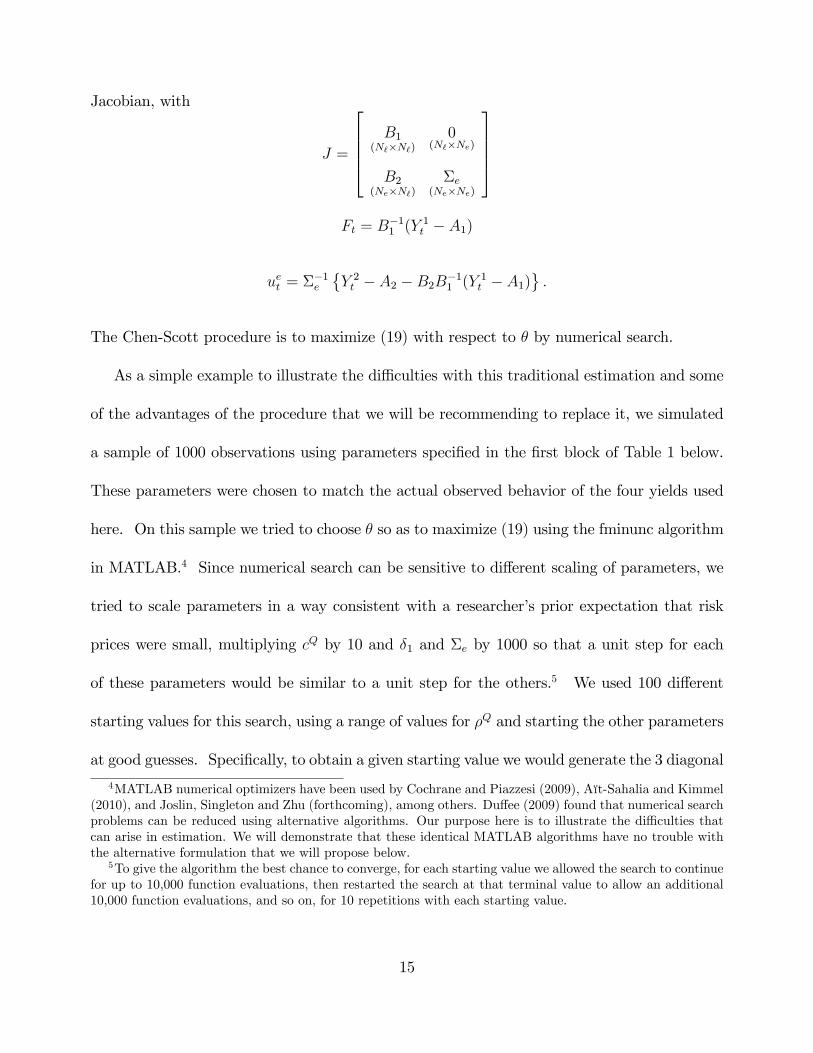
Jacobian, with
J =
26664B1
(N`�N`)0
(N`�Ne)
B2(Ne�N`)
�e(Ne�Ne)
37775Ft = B�1
1 (Y1t � A1)
uet = ��1e
�Y 2t � A2 �B2B
�11 (Y
1t � A1)
:
The Chen-Scott procedure is to maximize (19) with respect to � by numerical search.
As a simple example to illustrate the di¢ culties with this traditional estimation and some
of the advantages of the procedure that we will be recommending to replace it, we simulated
a sample of 1000 observations using parameters speci�ed in the �rst block of Table 1 below.
These parameters were chosen to match the actual observed behavior of the four yields used
here. On this sample we tried to choose � so as to maximize (19) using the fminunc algorithm
in MATLAB.4 Since numerical search can be sensitive to di¤erent scaling of parameters, we
tried to scale parameters in a way consistent with a researcher�s prior expectation that risk
prices were small, multiplying cQ by 10 and �1 and �e by 1000 so that a unit step for each
of these parameters would be similar to a unit step for the others.5 We used 100 di¤erent
starting values for this search, using a range of values for �Q and starting the other parameters
at good guesses. Speci�cally, to obtain a given starting value we would generate the 3 diagonal
4MATLAB numerical optimizers have been used by Cochrane and Piazzesi (2009), Aït-Sahalia and Kimmel(2010), and Joslin, Singleton and Zhu (forthcoming), among others. Du¤ee (2009) found that numerical searchproblems can be reduced using alternative algorithms. Our purpose here is to illustrate the di¢ culties thatcan arise in estimation. We will demonstrate that these identical MATLAB algorithms have no trouble withthe alternative formulation that we will propose below.
5To give the algorithm the best chance to converge, for each starting value we allowed the search to continuefor up to 10,000 function evaluations, then restarted the search at that terminal value to allow an additional10,000 function evaluations, and so on, for 10 repetitions with each starting value.
15

elements of �Q from U [0:5; 1] distributions, set o¤-diagonal elements to zero, and set the initial
guess for � equal to this value for �Q: We set the starting value for each element of �1 and �e
to 1.e-4, �0 = 0:0046 (the average short rate), and cQ = 0:
True values Global maximum Local 53cQ 0.0407 0.0135 0.5477 0.0416 0.0085 0.5316 -0.5562 0.0204 0.0527�Q 0.9991 0 0 0.9985 0 0 0.9986 0 0
0.0101 0.9317 0 0.0116 0.9328 0 0.0113 0.9316 00.0289 0.2548 0.7062 0.0219 0.2500 0.7202 0.0203 0.2438 0.7352
� 0.9812 0.0069 0.0607 0.9696 0.0141 0.0671 0.9794 0.0063 0.0840-0.0010 0.8615 0.1049 -0.0027 0.8533 0.1175 -0.0028 0.8380 0.12670.0164 0.1856 0.6867 0.0085 0.1985 0.6993 0.0333 0.1923 0.7202
�0 0.0046 0.0046 0.1344�1 1.729E-4 1.803E-4 4.441E-4 1.71E-4 1.71E-4 4.45E-4 1.72E-4 1.59E-4 4.54E-4�e 9.149E-5 9.105E-5 9.110E-5
eig(�) 0.9879 0.9341 0.6074 0.9734 0.9448 0.6040 1.000 0.9306 0.6070LLF 28110.4 28096.5
Table 1: Parameter values used for simulation and estimates associated with (1) the globalmaximum and (2) a representative point of local convergence.
In only 1 of these 100 experiments did the numerical search converge to the values that
we will establish below are indeed the true global MLE. These estimates, reported in the
second block of Table 1, in fact correspond very nicely to the true values from which this
sample was simulated. However, in 81 of the other experiments, the procedure satis�ed the
convergence criterion (usually coming from a su¢ ciently tiny change between iterations) at a
large range of alternative points other than the global maximum. The third block of Table
1 displays one of these. All such points are characterized by an eigenvalue of � being equal
or very close to unity; we will explain why this happens in the following section. For the
other 18 starting values, the search algorithm was unable to make any progress from the initial
starting values. Although very simple, this exercise helps convey some sense of the numerical
16

problems researchers have encountered �tting more complicated models such as we describe
in our next two examples.
2.3 Example 2: Macro �nance model with single lag (MF1).
It is of considerable interest to include observable macroeconomic variables among the factors
that may a¤ect interest rates, as for example in Ang and Piazzesi (2003), Ang, Dong and
Piazzesi (2007), Rudebusch and Wu (2008), Ang, Piazzesi and Wei (2006), and Hordahl,
Tristani and Vestin (2006). Our next two illustrative examples come from this class. We
�rst consider the unrestricted �rst-order macro factor model studied by Pericoli and Taboga
(2008). This model uses Nm = 2 observable macro factors, consisting of measures of the
in�ation rate and the output gap, which are collected in an (Nm � 1) vector fmt : These two
observable macroeconomic factors are allowed to in�uence yield dynamics in addition to the
traditional N` = 3 latent6 factors f `t ,
Ft(Nf�1)
=
26664fmt
(Nm�1)
f `t(N`�1)
37775 ;6Pericoli and Taboga evaluated a number of alternative speci�cations including di¤erent choices for the
number of latent factors N`; number of lags on the macro variables, and dependence between the latent andmacro factors. They refer to the speci�cation we discuss in the text as the M(3; 0; U) speci�cation, which isthe one that their tests suggest best �ts the data.
17

for Nf = Nm +N`: The P dynamics (1), Q dynamics (12), and short-rate equation (13) can
for this example be written in partitioned form as
fmt(Nm�1)
= cm + �mmfmt�1 + �m`f
`t�1 + �mmu
mt (20)
f `t(N`�1)
= c` + �`mfmt�1 + �``f
`t�1 + �`mu
mt + �``u
`t
fmt(Nm�1)
= cQm + �Qmmfmt�1 + �Qm`f
`t�1 + �mmu
Qmt (21)
f `t(N`�1)
= cQ` + �Q`mfmt�1 + �Q``f
`t�1 + �`mu
Qmt + �``u
Q`t
rt = �0 + �01mfmt + �01`f
`t : (22)
Pericoli and Taboga proposed the normalization conditions7 that �mm is lower triangular,
�`m = 0; �`` = IN` ; �1` � 0; and cQ` = 0:
Our empirical illustration of this approach will use t corresponding to quarterly data and
will take the 1-, 5-, and 10-year bonds to be priced without error (Y 1t = (y
4t ; y
20t ; y
40t )
0) and the
2-, 3-, and 7-year bonds to be priced with error (Y 2t = (y
8t ; y
12t ; y
28t )
0): Details of how the log
likelihood is calculated for this example are described in Appendix A.
7Pericoli and Taboga imposed f `0 = 0 as an alternative to the traditional c` = 0 or cQ` = 0, though we will
follow the rest of the literature here in using a more standard normalization.
18

2.4 Example 3: Macro �nance model with 12 lags (MF12).
A �rst-order VAR is not su¢ cient to capture the observed dynamics of output and in�ation.
For example, Ang and Piazzesi (2003) suggested that the best �t is obtained using a monthly
VAR(12) in the observable macro variables and a VAR(1) for the latent factors:8
fmt = �1fmt�1 + �2f
mt�2 + � � �+ �12f
mt�12 + �mmu
mt
f `t = c` + �``f`t�1 + �``u
`t:
Our empirical example follows Ang and Piazzesi in proxying the 2 elements of fmt with the
�rst principal components of a set of output and and a set of in�ation measures, respectively,
which factors have mean zero by construction. Ang and Piazzesi treated the macro dynamics
as independent of those for the unobserved latent factors, so that terms such as �`m and �m`
in the preceding example are set to zero.
Ang and Piazzesi (2003) further proposed the following identifying restrictions: �mm is
lower triangular, �`` = IN` ; c` = 0; �`` is lower triangular, and the diagonal elements of �`` are
in descending order. Further restrictions and details of the model and its likelihood function
are provided in Appendix B. In the speci�cation we replicate, Ang and Piazzesi postulated
that the short rate depends only on the current values of the macro factors:
rt = �0 + �0
1mfmt + �
0
1`f`t :
8Ang and Piazzesi refer to this as their Macro Model.
19
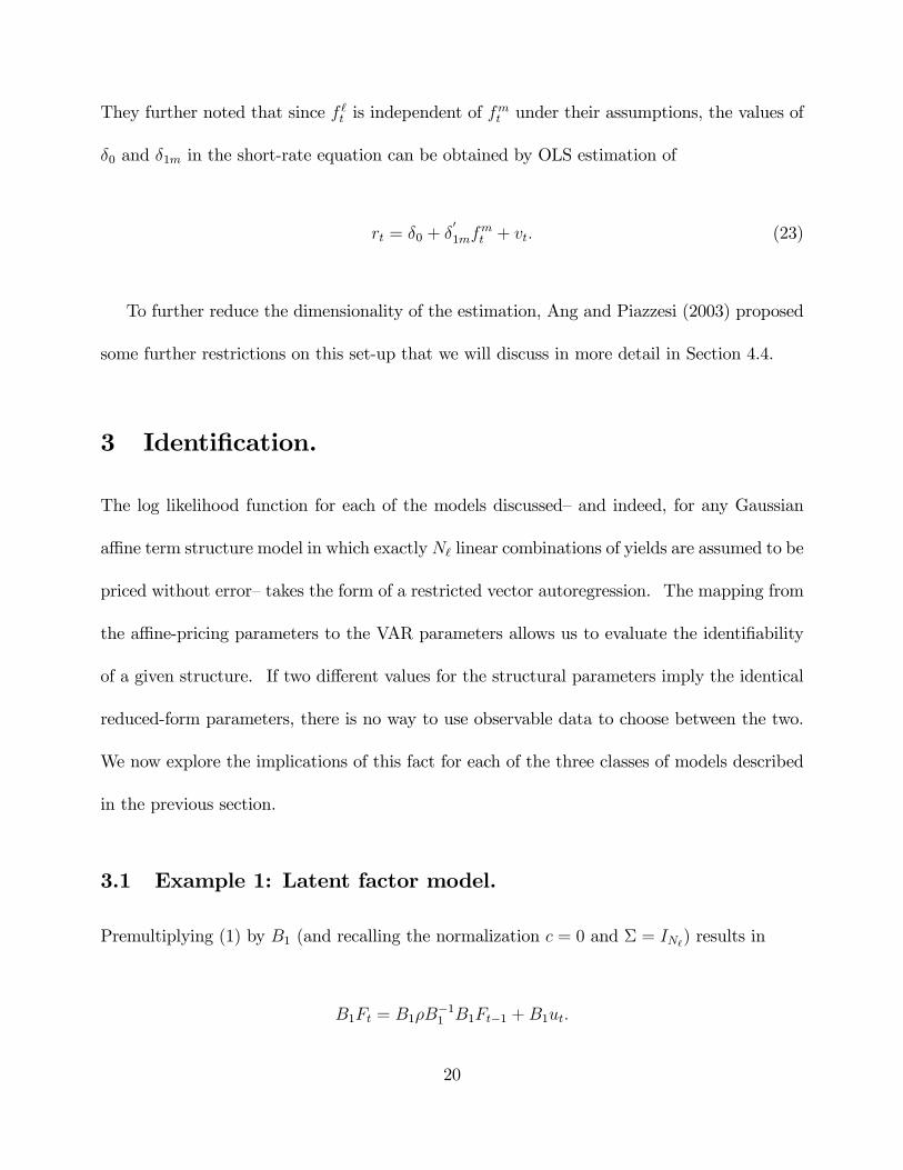
They further noted that since f `t is independent of fmt under their assumptions, the values of
�0 and �1m in the short-rate equation can be obtained by OLS estimation of
rt = �0 + �0
1mfmt + vt: (23)
To further reduce the dimensionality of the estimation, Ang and Piazzesi (2003) proposed
some further restrictions on this set-up that we will discuss in more detail in Section 4.4.
3 Identi�cation.
The log likelihood function for each of the models discussed�and indeed, for any Gaussian
a¢ ne term structure model in which exactlyN` linear combinations of yields are assumed to be
priced without error�takes the form of a restricted vector autoregression. The mapping from
the a¢ ne-pricing parameters to the VAR parameters allows us to evaluate the identi�ability
of a given structure. If two di¤erent values for the structural parameters imply the identical
reduced-form parameters, there is no way to use observable data to choose between the two.
We now explore the implications of this fact for each of the three classes of models described
in the previous section.
3.1 Example 1: Latent factor model.
Premultiplying (1) by B1 (and recalling the normalization c = 0 and � = IN`) results in
B1Ft = B1�B�11 B1Ft�1 +B1ut:
20

Adding A1 to both sides and substituting Y 1t = A1 +B1Ft establishes
Y 1t = A�1 + ��11Y
1t�1 + u�1t (24)
A�1 = A1 �B1�B�11 A1 (25)
��11 = B1�B�11 : (26)
Likewise the second block of (17) implies
Y 2t = A�2 + ��21Y
1t + u�2t (27)
A�2 = A2 �B2B�11 A1 (28)
��21 = B2B�11 (29)2664 u�1t
u�2t
3775 � N
0BB@2664 00
3775 ;2664 �1 0
0 �2
37751CCA (30)
�1 = B1B0
1 (31)
�2 = �e�0e: (32)
Equations (24) and (27) will be recognized as a restricted Gaussian VAR for Yt, in which
a single lag of Y 1t�1 appears in the equation for Y
1t and in which, after conditioning on the
contemporaneous value of Y 1t ; no lagged terms appear in the equation for Y
2t : Note that when
we refer to the reduced-form for this system, we will incorporate those exclusion restrictions
21

along with the restriction that �2 is diagonal.
Table 2 summarizes the mapping between the VAR parameters and the a¢ ne term struc-
ture parameters implied by equations (24)-(32).9 The number of VAR parameters minus
the number of structural parameters is equal to (Ne � 1)(N` + 1): Thus the structure is
just-identi�ed by a simple parameter count when Ne = 1 and overidenti�ed when Ne > 1:
Notwithstanding, the structural parameters can nevertheless be unidenti�ed despite the ap-
parent conclusion from a simple parameter count.
VAR No. of �e �Q �1 � cQ �0parameter elements Ne N`(N` + 1)=2 N` N2
` N` 1�2 Ne X��21 N`Ne X�1 N`(N` + 1)=2 X X��11 N2
` X X XA�2 Ne X X X XA�1 N` X X X X X
Table 2: Mapping between structural and reduced-form parameters for the latent factor model.
Consider �rst what happens at a point where one of the eigenvalues of � is unity, that
is, when the P -measure factor dynamics exhibit a unit root.10 This means that one of
the eigenvalues of B1�B�11 is also unity (B1�B�1
1 x = x for some nonzero x) requiring that
(IN` � B1�B�11 )x = 0; so the matrix IN` � B1�B
�11 is noninvertible. In this case, even if we
knew the true value of A�1, we could never �nd the value of A1 from equation (25). If A1 is
proposed as a �t for a given sample, then A1 + kx produces the identical �t for any k. Note
moreover from (16) that A1 and A2 are the only way to �nd out about cQ and �0; if we don�t
9The value of �1 turns out not to appear in the product ��21 = B2B
�11 :
10Note we have followed Ang and Piazzesi (2003) and Joslin, Singleton and Zhu (forthcoming), amongothers, in basing estimates on the likelihood function conditional on the �rst observation. By contrast, Chenand Scott (1993) and Du¤ee (2002) include the unconditional likelihood of the �rst observation as a device forimposing stationarity.
22
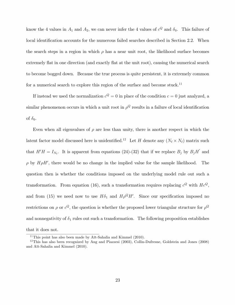
know the 4 values in A1 and A2; we can never infer the 4 values of cQ and �0. This failure of
local identi�cation accounts for the numerous failed searches described in Section 2.2. When
the search steps in a region in which � has a near unit root, the likelihood surface becomes
extremely �at in one direction (and exactly �at at the unit root), causing the numerical search
to become bogged down. Because the true process is quite persistent, it is extremely common
for a numerical search to explore this region of the surface and become stuck.11
If instead we used the normalization cQ = 0 in place of the condition c = 0 just analyzed, a
similar phenomenon occurs in which a unit root in �Q results in a failure of local identi�cation
of �0:
Even when all eigenvalues of � are less than unity, there is another respect in which the
latent factor model discussed here is unidenti�ed.12 Let H denote any (N`�N`) matrix such
that H 0H = IN` : It is apparent from equations (24)-(32) that if we replace Bj by BjH0and
� by H�H 0, there would be no change in the implied value for the sample likelihood. The
question then is whether the conditions imposed on the underlying model rule out such a
transformation. From equation (16), such a transformation requires replacing cQ with HcQ,
and from (15) we need now to use H�1 and H�QH 0: Since our speci�cation imposed no
restrictions on � or cQ; the question is whether the proposed lower triangular structure for �Q
and nonnegativity of �1 rules out such a transformation. The following proposition establishes
that it does not.11This point has also been made by Aït-Sahalia and Kimmel (2010).12This has also been recognized by Ang and Piazzesi (2003), Collin-Dufresne, Goldstein and Jones (2008)
and Aït-Sahalia and Kimmel (2010).
23

Proposition 1. Consider any (2� 2) lower triangular matrix:
�Q =
2664 �Q11 0
�Q21 �Q22
3775 :
Then for almost all (2�1) positive vectors �1; there exists a unique orthogonal matrix H other
than the identity matrix such that H�QH 0 is also lower triangular and H�1 > 0: Moreover,
H�QH 0 takes one of the following forms:
2664 �Q22 0
�Q21 �Q11
3775 or
2664 �Q22 0
��Q21 �Q11
3775 :
For �Q an (N` � N`) lower triangular matrix, there are N`! di¤erent lower triangular repre-
sentations, characterized by alternative orderings of the principal diagonal elements.
There thus exist 6 di¤erent parameter con�gurations that would achieve the same maxi-
mum for the likelihood function for the latent example explored in Section 2.2. The experiment
did not uncover them because the other di¢ culties with maximization were su¢ ciently severe
that for the 100 di¤erent starting values used, only one of these 6 con�gurations was reached.
Dai and Singleton (2000) and Singleton (2006) originally proposed lower triangularity of �
or �Q and nonnegativity of �1 as su¢ cient identifying conditions. Our proposition estab-
lishes that one needs a further condition such as �Q11 � �Q22 � �Q33 to have a globally identi�ed
structure.
Nevertheless, this multiplicity of global optima is a far less serious problem than the failure
of local identi�cation arising from a unit root. The reason is that any of the alternative
24
con�gurations obtained through these H transformations by construction has the identical
implications for bond pricing. By contrast, the inferences one would draw from Local 53 in
Table 1 are fundamentally �awed and introduce substantial practical di¢ culties for using this
class of models.
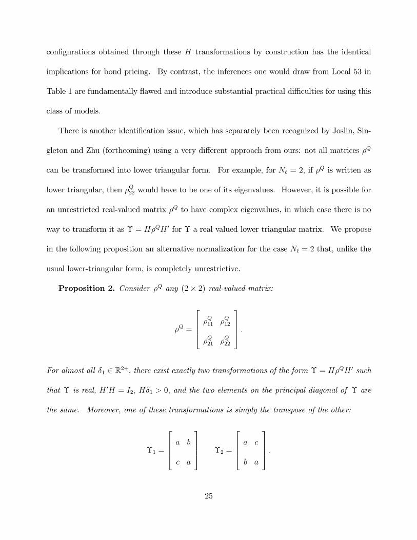
There is another identi�cation issue, which has separately been recognized by Joslin, Sin-
gleton and Zhu (forthcoming) using a very di¤erent approach from ours: not all matrices �Q
can be transformed into lower triangular form. For example, for N` = 2; if �Q is written as
lower triangular, then �Q22 would have to be one of its eigenvalues. However, it is possible for
an unrestricted real-valued matrix �Q to have complex eigenvalues, in which case there is no
way to transform it as � = H�QH 0 for � a real-valued lower triangular matrix. We propose
in the following proposition an alternative normalization for the case N` = 2 that, unlike the
usual lower-triangular form, is completely unrestrictive.
Proposition 2. Consider �Q any (2� 2) real-valued matrix:
�Q =
2664 �Q11 �Q12
�Q21 �Q22
3775 :
For almost all �1 2 R2+; there exist exactly two transformations of the form � = H�QH 0 such
that � is real, H 0H = I2; H�1 > 0; and the two elements on the principal diagonal of � are
the same. Moreover, one of these transformations is simply the transpose of the other:
�1 =
2664 a b
c a
3775 �2 =
2664 a c
b a
3775 :
25

Hence one approach for the N` = 2 case would be to choose the 3 parameters a; b; and c
so as to maximize the likelihood with
�Q =
2664 a b
c a
3775subject to the normalization b � c: This has the advantage over the traditional lower-
triangular formulation in that the latter imposes additional restrictions on the dynamics
(namely, lower-triangular �Q rules out the possibility of complex roots) whereas the � formu-
lation does not.
Unfortunately, it is less clear how to generalize this to larger dimensions. If �Q has complex
eigenvalues, these always appear as complex conjugates. Thus if one knew for the case N` = 3
that �Q contained complex eigenvalues, a natural normalization would be
�Q =
26666664�Q11 0 0
�Q21 a �Q23
�Q31 �Q32 a
37777775 (33)
with �Q23 � �Q32 The value of a is then uniquely pinned down by the real part of the complex
eigenvalues. However, if the eigenvalues are all real, this is a more awkward form than the
usual
�Q =
26666664�Q11 0 0
�Q21 �Q22 0
�Q31 �Q32 �Q33
37777775 (34)
26

with �Q11 � �Q22 � �Q33: The estimation approach that we propose below will instantly reveal
whether or not the lower triangular form (34) is imposing a restriction relative to the full-
information maximum likelihood unrestricted values. If (34) is determined not to impose
a restriction, one can feel con�dent in using the conventional parameterization, whereas if
it does turn out to be inconsistent with the estimated unrestricted dynamics, the researcher
should instead parameterize dynamics using (33).
3.2 Example 2: Macro �nance model with single lag.
We next examine the MF1 speci�cation of Pericoli and Taboga (2008). Calculations similar
to those for the latent factor model show the reduced form to be
fmt(Nm�1)
= A�m(Nm�1)
+ ��mm(Nm�Nm)
fmt�1 + ��m1(Nm�N`)
Y 1t�1 + u�mt (35)
Y 1t
(N`�1)= A�1
(N`�1)+ ��1m(N`�Nm)
fmt�1 + ��11(N`�N`)
Y 1t�1 + �1m
(N`�Nm)fmt + u�1t (36)
Y 2t
(Ne�1)= A�2
(Ne�1)+ ��2m(Ne�Nm)
fmt + ��21(Ne�N`)
Y 1t + u�2t: (37)
Once again it is convenient to include the contemporaneous value of fmt in the equation for
Y 1t and include contemporaneous values of both f
mt and Y 1
t in the equation for Y2t in order to
orthogonalize the reduced-form residuals u�jt; the bene�ts of this representation will be seen
in the next section. The mapping between structural and reduced-form parameters is given
27
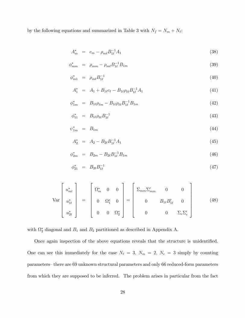
by the following equations and summarized in Table 3 with Nf = Nm +N`:
A�m = cm � �m`B�11` A1 (38)
��mm = �mm � �m`B�11` B1m (39)
��m1 = �m`B�11` (40)
A�1 = A1 +B1`c` �B1`�``B�11` A1 (41)
��1m = B1`�`m �B1`�``B�11` B1m (42)
��11 = B1`�``B�11` (43)
�1m = B1m (44)
A�2 = A2 �B2`B�11` A1 (45)
��2m = B2m �B2`B�11` B1m (46)
��21 = B2`B�11` (47)
Var
26666664u�mt
u�1t
u�2t
37777775 =
26666664�m 0 0
0 �1 0
0 0 �2
37777775 =26666664�mm�
0mm 0 0
0 B1`B01` 0
0 0 �e�0e
37777775 (48)
with �2 diagonal and B1 and B2 partitioned as described in Appendix A.
Once again inspection of the above equations reveals that the structure is unidenti�ed.
One can see this immediately for the case N` = 3; Nm = 2; Ne = 3 simply by counting
parameters�there are 69 unknown structural parameters and only 66 reduced-form parameters
from which they are supposed to be inferred. The problem arises in particular from the fact
28

VAR No. of �e �mm �Q �1 �m` �mm �`` �`m �0 cQ cm c`parameter elements Ne Nm(Nm + 1)=2 N
2f Nf NmN` N
2m N2
` N`Nm 1 Nm Nm N`�2 Ne X�m Nm(Nm + 1)=2 X �1m N`Nm X X��2m NeNm X X��21 NeN` X X�1 N`(N` + 1)=2 X X��m1 NmN` X X X��mm N2
m X X X X��11 N2
` X X X��1m N`Nm X X X XA�2 Ne X X X X XA�m Nm X X X X X X XA�1 N` X X X X X X X
Table 3: Mapping between structural and reduced-form parameters for the MF1 model.
that, for the example we have been discussing, the observable implications of the 30 structural
parameters in �Q and �1 are completely captured by the 27 values of �1m; �
�2m; �
�21; and
�1.
More fundamentally, the lack of identi�cation would remain with this structure no matter
how large the value of Ne: One can see this by verifying that the following transformation
is perfectly allowed under the stated normalization but would not change the value of any
reduced-form parameter: B1` ! B1`H0; c` ! Hc`; �m` ! �m`H
0; �`` ! H�``H0; �`m ! H�`m;
and B2` ! B2`H0; where H could be any (N` �N`) orthogonal matrix.
There is also a separate identi�cation problem arising from the fact that only maturi-
ties for which n is an even number are included in the observation set. This means that
only even powers of �Q appear in (15) and (16), which allows observationally equivalent sign
transformations through H as well.
29

3.3 Example 3: Macro �nance model with 12 lags.
Last we consider the MF12 example, for which the reduced form is
fmt(2�1)
= ��mm(2�24)
Fmt�1 + u�mt (49)
Y 1t
(3�1)= A�1 + ��1m
(3�24)Fmt�1 + ��11
(3�3)Y 1t�1 + �1m
(3�2)fmt + u�1t (50)
Y 2t
(2�1)= A�2 + ��2m
(2�24)Fmt + ��21
(2�3)Y 1t + u�2t (51)
��mm =
��1 �2 � � � �12
�A�1 = A1 �B1`�``B
�11` A1
��1m(3�24)
=
"B(1)1m
(3�22)0
(3�2)
#� B1`�``B
�11`
(3�3)
"B(0)1m
(3�2)B(1)1m
(3�22)
#��11 = B1`�``B
�11`
�1m = B(0)1m
A�2 = A2 �B2`B�11` A1
��2m = B2m �B2`B�11` B1m
��21 = B2`B�11`
Var
0BBBBBB@
26666664u�mt
u�1t
u�2t
37777775
1CCCCCCA =
26666664�m 0 0
0 �1 0
0 0 �2
37777775 =26666664�mm�
0mm 0 0
0 B1`B01` 0
0 0 �e�0e
37777775with �2 again diagonal and details on the partitioning of B1 and B2 in Appendix B. Table
4 summarizes the mapping between reduced-form and structural parameters. Note that the
30

only reduced-form parameters relevant for inference about the 6 elements of �0 and � are the
5 values for A�1 and A�2; establishing that these structural parameters are in fact unidenti�ed.
One might have thought that perhaps �0 could be inferred separately from the OLS regression
(23), freeing up the parameters A�1 and A�2 for estimation solely of �. However, this is not the
case, since the short-term interest rate is the same dependent variable in both regression (23)
and in the �rst OLS regression from which A�1 is inferred. Another way to see this is to note
that at most what one can expect to uncover from the 5 values of A�1 and A�2 are the 5 values
of A1 and A2: The �rst element of A1 is exactly equal to �0, so even if �0 were known a priori,
the most that one could infer from A1 and A2 is 4 other parameters. Hence A1 and A2 would
not be su¢ cient to uncover the 5 unknowns in � even if �0 were known with certainty.
VAR No. of �e �mm �1;:::;12 �mm �1m �`` �`` �1` �0 �parameter elements 2 3 48 4 2 6 9 3 1 5�2 2 X�m 3 X��mm 48 X �1m 6 X X X��21 6 X X X�1 6 X X X��11 9 X X X��2m 48 X X X X X X��1m 72 X X X X X XA�2 2 X X X X X X X X XA�1 3 X X X X X X X X X
Table 4: Mapping between structural and reduced-form parameters for the MF12 model.
Ang and Piazzesi�s (2003) Macro Model with its proposed identifying restrictions thus turns
out to be unidenti�ed at all points of the parameter space. In their empirical analysis, Ang and
Piazzesi imposed an additional set of restrictions that were intended to improve estimation
e¢ ciency, though as we have just seen some of these are necessary for identi�cation. We
31

discuss these further in Section 4.4 below.
4 Estimation.
The reduced-form parameters are trivially obtained via OLS. Hence a very attractive alter-
native to numerical maximization of the log likelihood function directly with respect to the
structural parameters � is to let OLS do the work of maximizing the likelihood with respect
to the reduced-form parameters, and then translate these into their implications for �: We
demonstrate in this section how this can be done.
4.1 Minimum-chi-square estimation.
Let � denote the vector consisting of reduced-form parameters (VAR coe¢ cients and nonre-
dundant elements of the variance matrices), L(�;Y ) denote the log likelihood for the entire
sample, and � = argmaxL(�;Y ) denote the full-information-maximum-likelihood estimate.
If R is a consistent estimate of the information matrix,
R = �T�1E�@2L(�;Y )@� @�0
�
then we could test the hypothesis that � = g(�) for � a known vector of parameters by
calculating the usual Wald statistic
T [� � g(�)]0 R [� � g(�)] (52)
32

which would have an asymptotic �2(q) distribution under the null hypothesis where q is the
dimension of �. Rothenberg (1973, p. 24) noted that one could also use (52) as a basis for
estimation by choosing as an estimate � the value that minimizes this chi-square statistic.
Following Rothenberg (1973, pp. 24-25), we can obtain asymptotic standard errors by
considering the linear approximation g(�) ' +�� for � = @g(�)=@�0j�=�0 and = g(�0)���0
where �p! �0 and we assume there exists a value of �0 for which the true model satis�es
g(�0) = �0: De�ne the linearized minimum-chi-square estimator ��as the solution to
min�
T [� � � ��]0R [� � � ��] ;
that is, ��satis�es �0R(� � � ���) = 0 or �
�= (�0R�)�1�0R(� � ): Since
pT (� �
�0)L! N(0; R�1); it follows that
pT (�
� � �0)L! N (0; [�0R�]�1) : Hence our proposal is to
approximate the variance of � with T�1(�0R�)�1 for � = @g(�)=@�0j�=� :
We show in Appendix E that this is in fact identical to the usual asymptotic variance
for the MLE as obtained from second derivatives of the log likelihood function directly with
respect to �: In other words, the MCSE and MLE are asymptotically equivalent, and the
MCSE inherits all the asymptotic optimality properties of the MLE. If in a particular sample
the MCSE and MLE di¤er, there is no basis for claiming that one has better properties than
the other.
In the case of a just-identi�ed model, the minimum value attainable for (52) is zero, in
which case one can without loss of generality simply minimize
[� � g(�)]0 [� � g(�)] : (53)
33

Note that in this case, if the optimized value for this objective is zero, then � is numeri-
cally identical to the value that achieves the global maximum of the likelihood written as a
function of �: Although �MCSE in this case is identical to �MLE; arriving at the estimate
by the minimum-chi-square algorithm has two big advantages over the traditional brute-force
maximization of the likelihood function. First, one knows instantly whether � corresponds
to a global maximum of the original likelihood surface simply by checking whether a zero
value is achieved for (53). By contrast, under the traditional approach, one has to try hun-
dreds of starting values to be persuaded that a global maximum has been found, and even
then cannot be sure. A second advantage is that minimization of (52) or (53) is far simpler
computationally than brute-force maximization of the original likelihood function.
In addition, the greater computational ease makes calculation of small-sample con�dence
intervals feasible. The models considered here imply a reduced form that can be written in
companion form as
Yt = k + �Yt�1 + �Y ut
for Yt the (N � 1) vector of observed variables (yields, macro variables, and possible lags
of macro variables) and ut � N(0; IN); where the parameters k; �, and �Y are known
functions of �: We can then obtain bootstrap con�dence intervals for � as follows. For
arti�cial sample j, we will generate a sequence fu(j)t gTt=1 of N(0; IN) variables for T the
original sample size, and then recursively generate Y (j)t = k(�) + �(�)Y
(j)t�1 + �Y (�)u
(j)t for
t = 1; 2; :::; T; starting from Y(j)0 = Y0; the initial value from the original sample, and using
the identical parameter values k; �, and �Y (as implied by the original �) for each sample
j. On sample j we �nd the FIML estimate �(j) on that arti�cial sample and then calculate
34

�(j)= argmin
�Th�(j) � g(�)
i0R(j)
h�(j) � g(�)
i: We generate a sequence j = 1; 2; :::; J of such
samples, from which we could calculate 95% small-sample con�dence intervals for each element
of �: The small-sample standard errors for parameter i reported in the following section were
calculated fromqJ�1
PJj=1(�
(j)
i;MCSE � �i)2 where �i is the MCSE estimate for the original
sample (whose original FIML � was used to generate each arti�cial sample j) and �(j)
i;MCSE is
the minimum-chi-square estimate for arti�cial sample j.
We now illustrate these methods and their advantages in detail using the examples of a¢ ne
term structure models discussed above.
4.2 Example 1: Latent factor model.
In the case of Ne = 1; the latent factor model is just-identi�ed, making application of
minimum-chi-square estimation particularly attractive. The reduced-form parameter vec-
tor here is
� =
�vec��
A�1 ��11
�0��0; [vech(�1)]
0;
�vec��
A�2 ��21
�0��0; [diag(�2)]
0
!0
where vec(X) stacks the columns of the matrix X into a vector. If X is square, vech(X) does
the same using only the elements on or below the principal diagonal, and diag(X) constructs a
vector from the diagonal elements ofX. Because u�1t and u�2t are independent, full-information-
maximum-likelihood (FIML) estimation of � is obtained by treating the Y1 and Y2 blocks
separately. Since each equation of (24) has the same explanatory variables, FIML for the
ith row of [A�1; ��11] is obtained by OLS regression of Y
1it on a constant and Y
1t�1; with
�1 the
35

matrix of average outer products of those OLS residuals:
�1 = T�1TXt=1
(Y 1t � A�1 � �
�11Y
1t�1)(Y
1t � A�1 � �
�11Y
1t�1)
0:
FIML estimates of the remaining elements of � are likewise obtained from OLS regressions
of Y 2it on a constant and Y
1t :
The speci�c mapping in Table 2 suggests that we can use the following multi-step algorithm
to minimize (53) for the latent factor model with N` = 3 and Ne = 1:
Step 1. The estimate of �e is obtained analytically from the square root of �2:
Step 2. The estimates of the 9 unknowns in �Q and �1 are found by numerically solving
the 9 equations in (29) and (31)
[B2(�Q; �1)][B1(�
Q; �1)]0 = �
�21
�1
[B1(�Q; �1)][B1(�
Q; �1)]0 = �1:
Speci�cally, we do this by letting13 �2 = (hvec(�
�21
�1)i0; [vech(�1)]
0)0 and g2(�Q; �1) = ([vec(B2B01)]
0;
[vech(B1B01)]
0)0 and �nding �Q and �1 by numerical minimization of [�2 � g2(�Q; �1)]
0[�2 �
g2(�Q; �1)]:
13To assist with scaling for numerical robustness, we multiplied each equation in step 2 by 1200�1:e+7 andthose in step 4 below by 1.e+8. If we were minimizing (52) directly one would automatically achieve optimalscaling by using R in place of a constant k times the identity matrix as here. However, our formulation takesadvantage of the fact that the elements of � can be rearranged in order to avoid inversion of B1 inside thenumerical optimization, in which case R is no longer the optimal weighting matrix. The minimization wasimplemented using the fsolve command in MATLAB. We also multiplied �1 by 1000 to improve numericalrobustness.
36

Step 3. The estimate of � can then be obtained analytically from (26):
� = B�11 �
�11B1 (54)
where B1 is known from Step 2.
Step 4. Numerically solve the 4 unknowns in �0 and cQ from the 4 equations in A�1 and
A�2 using (25) and (28):
�I3 � B1�B
�11
�A1(�0; c
Q; �Q; �1) = A�1
A2(�0; cQ; �Q; �1)� B2B
�11 A1(�0; c
Q; �Q; �1) = A�2:
Although Steps 2 and 4 involve numerical minimization, these are computationally far sim-
pler problems than that associated with traditional brute-force maximization of the likelihood
function with respect to the full vector �. To illustrate this, we repeated the experiment
described in Section 2.2 with the same 100 starting values. Whereas we saw in Section 2.2
that only one of these e¤orts found the global maximum under the traditional approach, with
our method all 100 converge to the global MLE in one of the 6 con�gurations that are observa-
tionally equivalent for the original normalization. One of the reasons for the greater robustness
is that the critical stumbling block for the traditional method�numerical search over ��is
completely avoided since in our approach (54) is solved analytically. Another is that cQ and
uncertainties about its scale are completely eliminated from the core problem of estimation of
�Q and �1:
37

Joslin, Singleton and Zhu (forthcoming) have recently proposed a promising alternative
parameterization of the pure latent a¢ ne models that shares some of the advantages of our
approach. They parameterize the system such that A�1 and ��11 in (24) are taken to be
the direct objects of interest, and as in our approach, estimate these directly with OLS.
But whereas our approach also uses the OLS estimates of A�2 and ��21 in (27) to uncover
the remaining a¢ ne-pricing parameters, their approach �nds these by maximizing the joint
likelihood function of Y1 and Y2. Although they report that the second step involves no
numerical di¢ culties, our experience is that while it o¤ers a signi�cant improvement over the
traditional method, it is still susceptible to some of the same problems. For example, we
repeated the experiment described above with the same data set and same starting values for
�0 and the 3 unknown diagonal elements in �Q that appear in their parameterization as we
used in the simulations described above, starting the search for �1 from the OLS estimates as
they recommend. We found that the algorithm found the global maximum in 54 out of the
100 trials14, but got stuck in regions with diagonal elements of �Q equal to unity in the others,
in a similar failure of local identi�cation that we documented above can plague the traditional
approach.
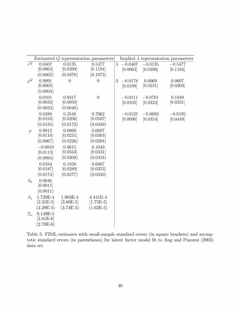
We applied our method directly to the Ang and Piazzesi interest rate data described in
more detail in Section 4.4 below. Table 5 reports the resulting minimum-chi-square estimates
(identical in this case to the full-information-maximum-likelihood estimates). The table also
reports asymptotic standard errors in parentheses and small-sample standard errors in square
brackets. The latter were calculated by applying our method to each of 1000 separate data
14To assist the numerical search, we multiplied �1 by 1000. Without this scaling, the searches only succeededin �nding the global maximum in 14 of the 100 trials.
38

sets, each generated from the vector autoregression estimated from the original data set. Note
that the fact that we can verify with certainty that the global maximum has been found on
each of these 1000 simulated data sets is part of what makes calculation of small-sample
standard errors feasible and attractive. Finding the FIML estimate on 1000 data sets takes
about 90 seconds on a PC. For this example, we �nd that the asymptotic standard errors
provide an excellent approximation to the true small-sample values.
Although our original inference was conducted in terms of a Q representation, we report
the implied � representation values in the right-hand columns of Table 5, since that is the
form in which parameter estimates are often reported for these models. Our suggestion is
that the approach we illustrate here, of beginning with a completely unrestricted model to
see which parameters appear to be most signi�cant, has many advantages over the traditional
approach15 in which sundry restrictions are imposed at a very early stage, partly in order to
assist with identi�cation and estimation.
4.3 Example 2: Macro �nance model with single lag.
We also applied this procedure to estimate parameters for our MF1 example using a slightly
di¤erent quarterly data set from Pericoli and Taboga. We used constant-maturity Treasury
yields as of the �rst day of the quarter, dividing the numbers as usually reported by 400 in
order to convert to units of quarterly yield on which formulas such as (14) are based. We
estimated in�ation from the 12-month percentage change in the CPI and the output gap by
applying the Hodrick-Prescott �lter with � = 1600 to 100 times the natural log of real GDP.
15See for example Du¤ee (2002) and Duarte (2004).
39
Estimated Q representation parameters Implied � representation parameterscQ 0:0407
[0:0063](0:0062)
0:0135[0:0399](0:0378)
0:5477[0:1194](0:1073)
� �0:0407[0:0063]
�0:0135[0:0399]
�0:5477[0:1194]
�Q 0:9991[0:0005](0:0004)
0 0 � �0:0178[0:0109]
0:0069[0:0231]
0:0607[0:0303]
0:0101[0:0033](0:0032)
0:9317[0:0050](0:0046)
0 �0:0111[0:0102]
�0:0701[0:0323]
0:1049[0:0331]
0:0289[0:0193](0:0185)
0:2548[0:0206](0:0172)
0:7062[0:0507](0:0439)
�0:0125[0:0090]
�0:0693[0:0354]
�0:0195[0:0449]
� 0:9812[0:0110](0:0067)
0:0069[0:0231](0:0226)
0:0607[0:0303](0:0294)
�0:0010[0:0113](0:0094)
0:8615[0:0343](0:0309)
0:1049[0:0331](0:0318)
0:0164[0:0187](0:0174)
0:1856[0:0289](0:0277)
0:6867[0:0353](0:0350)
�0 0:0046[0:0011](0:0011)
�1 1.729E-4[2.31E-5](2.28E-5)
1.803E-4[3.80E-5](3.74E-5)
4.441E-4[1.75E-5](1.62E-5)
�e 9.149E-5[2.81E-6](2.70E-6)
Table 5: FIML estimates with small-sample standard errors (in square brackets) and asymp-totic standard errors (in parentheses) for latent factor model �t to Ang and Piazzesi (2003)data set.
40

Data run from 1960:Q1 to 2007:Q1 and were obtained from the FRED database of the Federal
Reserve Bank of St. Louis.
If we impose 3 further restrictions on �Q`` relative to the original formulation, the MF1
model presented above would be just-identi�ed in terms of parameter count, for which we
would logically again simply try to invert the reduced-form parameter estimates to obtain
the FIML estimates of the structural parameters. Once again orthogonality of the residuals
across the three blocks of (35) through (37) means FIML estimation can be done on each block
separately, and within each block implemented by OLS equation by equation. Our estimation
procedure on this system is then as follows.
Step 1. The fmt and Y 2t variance parameters are obtained analytically from (48), that is,
�mm from the Cholesky factorization of �m and �e from the square root of �2:
Step 2. Using (44), (46), (48), and (47), choose the values of �Q and �1 so as to solve the
following equations numerically16:
B1m(�Q; �1) =
�1m
B2m(�Q; �1) = �
�2m + �
�21
�1m
vechn�B1`(�
Q; �1)� �B1`(�
Q; �1)�0o
= vech��1
��B2`(�
Q; �1)� �B1`(�
Q; �1)�0= �
�21
�1:
We initially tried to solve this system for �Q`` of the lower-triangular form (34), but found no
16To improve accuracy of the numerical algorithm, we multiplied the last two equations by 400 and thenthe whole set of equations by 1.e+7. The parameter �1 was also scaled by 100.
41
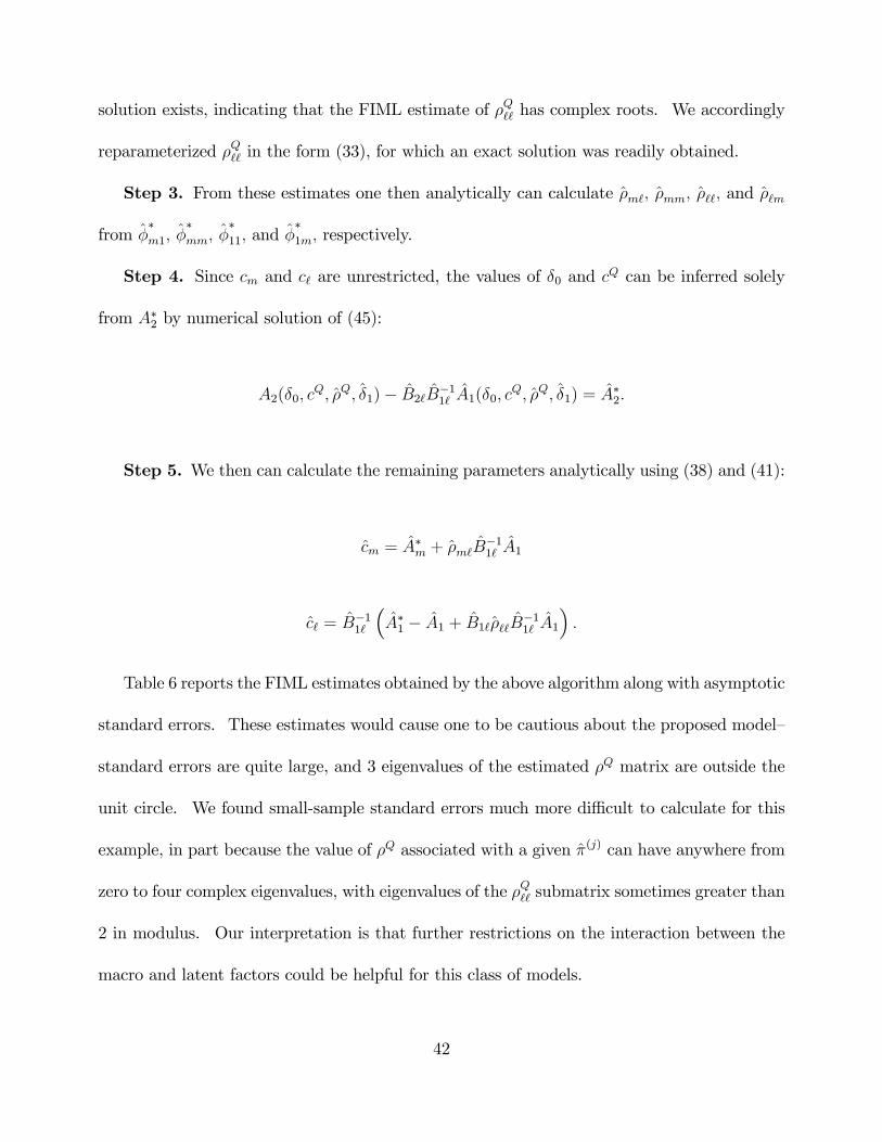
solution exists, indicating that the FIML estimate of �Q`` has complex roots. We accordingly
reparameterized �Q`` in the form (33), for which an exact solution was readily obtained.
Step 3. From these estimates one then analytically can calculate �m`; �mm; �``; and �`m
from ��m1; �
�mm; �
�11; and �
�1m; respectively.
Step 4. Since cm and c` are unrestricted, the values of �0 and cQ can be inferred solely
from A�2 by numerical solution of (45):
A2(�0; cQ; �Q; �1)� B2`B
�11` A1(�0; c
Q; �Q; �1) = A�2:
Step 5. We then can calculate the remaining parameters analytically using (38) and (41):
cm = A�m + �m`B�11` A1
c` = B�11`
�A�1 � A1 + B1`�``B
�11` A1
�:
Table 6 reports the FIML estimates obtained by the above algorithm along with asymptotic
standard errors. These estimates would cause one to be cautious about the proposed model�
standard errors are quite large, and 3 eigenvalues of the estimated �Q matrix are outside the
unit circle. We found small-sample standard errors much more di¢ cult to calculate for this
example, in part because the value of �Q associated with a given �(j) can have anywhere from
zero to four complex eigenvalues, with eigenvalues of the �Q`` submatrix sometimes greater than
2 in modulus. Our interpretation is that further restrictions on the interaction between the
macro and latent factors could be helpful for this class of models.
42

cQ 0:0306(0:5291)
�0:0458(1:1382)
0 0 0
c �0:1028(0:4951)
0:2414(0:4672)
�0:9632(7:2480)
�1:5301(1:4128)
2:4063(4:4009)
�Q 0:7725(0:2895)
0:2933(0:2801)
0:0436(1:0688)
�0:2138(0:1332)
�0:3565(0:3900)
�0:3933(0:3857)
1:2411(0:3706)
0:2376(0:2437)
�0:0197(0:1470)
�0:0574(0:5579)
0:2036(0:3691)
�0:2046(0:3852)
0:8579(0:1435)
0 0
�0:1035(0:2083)
0:1035(0:2373)
�0:0054(0:5723)
0:8826(0:0672)
�0:1926(0:1464)
0:1001(0:6387)
�0:1415(0:6661)
0:0223(0:1215)
0:0303(0:0810)
0:8826(0:0672)
� 0:9461(0:0325)
0:2203(0:0508)
�0:0428(0:2005)
�0:0210(0:0456)
0:0639(0:1531)
0:0002(0:0310)
0:8735(0:0487)
�0:0435(0:1618)
�0:0233(0:0538)
�0:0517(0:1555)
0:0932(0:3903)
0:1683(0:1686)
0:8203(0:6723)
�0:0844(0:2453)
0:1378(1:0303)
�0:0827(0:1190)
0:0852(0:1295)
�0:1110(0:3430)
0:8715(0:1127)
0:0978(0:2066)
0:1220(0:2649)
0:0449(0:5693)
0:0756(1:0167)
0:0555(0:1468)
0:4728(0:7418)
�0 �0:0082(0:0062)
�1 6.86E-4(2.88E-4)
1.02E-3(3.03E-4)
2.03E-3(2.35E-3)
1.92E-4(1.33E-3)
7.67E-4(6.31E-3)
�e 2.02E-4(1.29E-5)
1.87E-4(1.19E-5)
1.09E-4(6.97E-6)
�mm 0:6996(0:0448)
0
0:1174(0:0604)
0:6617(0:0424)
Table 6: FIML estimates and asymptotic standard errors for the MF1 model.
43

4.4 Example 3. Macro �nance model with 12 lags.
Here our data set follows Ang and Piazzesi (2003) as closely as possible, using zero-coupon
bond yields with maturities of 1, 3, 12, 36 and 60 months from CRSP monthly treasury �le,
each divided by 1200 to quote as monthly fractional rates. We obtained two groups of monthly
US macroeconomic key indicators, seasonally adjusted if applicable, from Datastream. The
�rst group consists of various in�ation measures which are based on the CPI, the PPI of �nished
goods, and the CRB Spot Index for commodity prices. The second group contains variables
that capture real activity: the Index of Help Wanted Advertising, Unemployment Rates, the
growth rate of Total Civilian Employment and the growth rate of Industrial Production. All
growth rates and in�ation rates are measured as the di¤erence in logs of the monthly index
value between dates t and t�12. We �rst normalized each series separately to have zero mean
and unit variance, then extracted the �rst principal component of each group, designated the
�in�ation�and �real activity�indices, respectively, with each index having zero mean and unit
variance by construction. The sample period for yields is from December 1952 to December
2000, and that for the macro indices is from January 1952 to December 2000. We assume
that 1-, 12- and 60-month yields are priced exactly, and 3- and 36-month yields are priced
with error (Ne = 2). We use the Ang and Piazzesi (2003) Macro Model with their additional
proposed zero restrictions to illustrate minimum-chi-square estimation for an overidenti�ed
model.
The reduced-form equations (49)-(51) form 3 independent blocks. If we interpret Y mt =
44

fmt , we can write the structure of block i for i = 1; 2;m as
Y it
(qi�1)= �0i
(qi�ki)xit(ki�1)
+ u�it(qi�1)
u�it � N(0;�i ):
The information matrix for the full system of reduced-form parameters is
R =
26666664Rm 0 0
0 R1 0
0 0 R2
37777775where as in Magnus and Neudecker (1988, p. 321)
Ri =
2664 ��1i T�1PT
t=1 xitx0it 0
0 (1=2)D0qi
���1i ��1i
�Dqi
3775for DN the N2 �N(N + 1)=2 duplication matrix satisfying DNvech() = vec():
The structural parameters �e appear only in the last half of the third block, no other
parameters appear in this block, and these 2 structural parameters are just-identi�ed by
the 2 diagonal elements of �2: Thus the minimum-chi-square estimates of �e are obtained
immediately from the square roots of diagonal elements of �2. The structural parameters
�1; :::; �12 appear directly in the �rst block and, through �Q; in the second and third blocks
as well, so FIML or minimum-chi-square estimation would exploit this. However, to reduce
dimensionality, we follow Ang and Piazzesi in replacing �2; :::; �12 where they appear in �Q with
45

the OLS estimates �2; :::; �12: In order to try to replicate their setting as closely as possible,
we also follow their procedure of imposing �1m on the basis of OLS estimation of (23). Hence
the minimum-chi-square analog to their problem is to minimize an expression of the form of
(52) with
� =
�hvec��1
�i0;hvech
��1
�i0;hvec��2
�i0�0(55)
R =
26666664��11 T�1
PTt=1 x1tx
01t 0 0
0 (1=2)D03
���11 ��11
�D3 0
0 0 ��12 T�1PT
t=1 x2tx02t
37777775x1t = (1; F
m0t�1; Y
10t�1; f
m0t )
0
x2t = (1; Fm0t ; Y 10
t )0
�0
i =
TXt=1
Y it x
0
it
! TXt=1
xitx0
it
!�1for i = 1; 2
�1 = T�1TXt=1
�Y 1t � �
0
1x1t
��Y 1t � �
0
1x1t
�0
�2 = T�1TXt=1
26666664[u2t(1)]
2 � � � 0
......
...
0 � � � [u2t(Ne)]2
37777775with u2t(j) the jth element of Y 2
t � �02x2t:
Ang and Piazzesi also imposed a further set of restrictions on parameters, setting parame-
ters with large standard errors as estimated in their �rst stage to zero. Their understanding
was that the purpose of these restrictions was to improve e¢ ciency, though we saw in Section
46

3.3 that some of these restrictions are in fact necessary in order to achieve identi�cation. Our
purpose here is to illustrate the minimum-chi-squared method on an overidenti�ed structure,
and we therefore attempt to estimate their �nal proposed structure using our method. The
additional parameters that Ang and Piazzesi �xed at zero include the (2,1) and (3,1) elements
of �`` (which recall was already lower triangular), the (1,2), (2,2), (3,2) and (1,3) elements of
�``, both elements in �m, and the 2nd and 3rd elements of �`. Our goal is then to minimize
(52) with respect to the 17 remaining unknown parameters, 1 in �`; 4 in �mm, 5 in �``, 4 in
�``, and 3 in �1`:17
The results of this estimation for 100 di¤erent starting values are reported in Table 7.
Our procedure uncovered three local minima to the objective function. The parameters we
report as Local1 correspond to the values reported in Table 6 of Ang and Piazzesi. The
small di¤erences between our estimates and theirs are due to some slight di¤erences between
the data sets and the fact that, in an overidenti�ed structure, the minimum-chi-square and
maximum-likelihood estimates are not numerically identical. Our procedure establishes that
the estimates reported by Ang and Piazzesi in fact represent only a local maximum of the
likelihood�both the estimates we report as Local2 and Global achieve substantially higher
values for the log likelihood function relative to Local1. Moreover, the di¤erences between
17 We made one other slight change in parameterization that may be helpful. Since �`` always enterseither the minimum-chi-squared calculations or the original maximum likelihood estimation in the form ofhigh powers of the matrix �Q`` = �`` � �``; the algorithms will be better behaved numerically if the unknownelements of �Q`` rather than those of �`` are taken to be the object of interest. Speci�cally, for this examplewe implemented this subject to the proposed restrictions by parameterizing
�`` =
24 �1 0 00 �2 00 �3 �4
35 �Q`` =
24 �5 0 0�6 �2 �7�8 �3 �9
35 ;and then translated back in terms of the implied values for �`` for purposes of reporting values in Table 7.
47

estimates in terms of the pricing of risk are substantial. In the original reported Ang and
Piazzesi estimates, an increase in in�ation lowers the price of in�ation risk and raises the price
of output risk, whereas the values implied by Global reverse these signs. This is consistent
with their �nding that the prices of observable macro risk behave very di¤erently between
their Macro Model and Macro Lag Model speci�cations�we �nd they also di¤er substantially
across alternative local maxima of the log likelihood function even within their single Macro
Model speci�cation. Note that the large prices of risk for these higher local maxima can make
them easy to miss with conventional estimation and conventional starting values of zero price
of risk.
Global Local1 Local2�`` 0.9921 0 0 0.9918 0 0 0.9920 0 0
0 0.9462 0 0 0.9412 0 0 0.9437 00 -0.0034 0.9021 0 -0.0095 0.7712 0 -0.0032 0.9401
�1` 1.11E-04 4.27E-04 1.98E-04 1.09E-04 4.30E-04 1.92E-04 1.22E-04 4.26E-04 1.92E-04�` -0.0409 0 0 -0.0441 0 0 -0.0388 0 0
�mm 2.8783 0.4303 -0.3430 0.1474 1.5633 0.1341-6.1474 -0.8744 1.7675 -0.0607 16.0624 7.4290
�`` -0.0048 0 0 -0.0045 0 0 -0.0056 0 0-0.0445 0 0.2910 -0.0474 0 0.2881 -0.0423 0 0.3000-0.0322 0 0.3687 -0.0331 0 0.2110 -0.0299 0 0.4120
�2 462.15 530.69 503.10LLF 20703 20668 20679
Frequency 14 84 2
Table 7: Three local minima for the chi-square objective function for the restricted MF12speci�cation.
Another bene�t of the minimum-chi-square estimation is that the value for the objective
function itself gives us an immediate test of the various overidentifying restrictions. There
are 152 parameters in the reduced form vector � in (55). The 17 estimated elements of � then
leave 135 degrees of freedom. The 1% critical value for a �2(135) variable is 176. Thus the
48

observed minimum value for our objective function (462.15) provides overwhelming evidence
that the restrictions imposed by the model are inconsistent with the observed data.
5 Conclusion.
We have characterized a¢ ne term structure models entirely in terms of their implications for
the parameters of a vector autoregression in observed variables. In addition to helping to
understand exactly what features of the data led to the particular asset-pricing parameter
estimates, this perspective allows us to evaluate the identi�ability of a proposed structure.
We demonstrated that a failure of local or global identi�cation can complicate traditional
estimation e¤orts, leading researchers to impose somewhat arbitrary restrictions in order to
obtain estimates and in other cases miss the true global maximum of the likelihood function.
We proposed an alternative estimation philosophy based on minimum-chi-square estimation,
which lets OLS �nd an unrestricted maximum of the likelihood surface and backs out from the
OLS estimates the optimal implied values for the structural parameters of interest. Among
other bene�ts, this approach makes it feasible in some cases to calculate small-sample standard
errors, instantly know whether estimates represent a global or only a local optimum, and
recognize whether a given structure is unintentionally restricting the class of possible a¢ ne
term structure models.
By showing how to recognize an unidenti�ed structure, greatly reducing the computational
burden of estimation, and providing an immediate speci�cation test of any proposed restric-
tions, we hope that our methods will help to make these models a more e¤ective tool for
49

research in macroeconomics and �nance.
References
Aït-Sahalia, Yacine and Robert L. Kimmel, �Estimating A¢ ne Multifactor Term Struc-
ture Models Using Closed-Form Likelihood Expansions,�Journal of Financial Economics,
2010, 98.
Ang, Andrew and Monika Piazzesi, �A no-arbitrage vector autoregression of term struc-
ture dynamics with macroeconomic and latent variables,�Journal of Monetary Economics,
2003, 50, 745�787.
, , and Min Wei, �What does the yield curve tell us about GDP growth,�Journal of
Econometrics, 2006, 131, 359�403.
, Sen Dong, and Monika Piazzesi, �No-arbitrage Taylor rules,�2007. National Bureau
of Economic Research, Working paper no. 13448.
Bauer, Michael D., �Term premia and the news.�PhD dissertation, University of California,
San Diego 2009.
Beechey, Meredith J. and Jonathan H. Wright, �The high-frequency impact of news
on long-term yields and forward rates: Is it real?,�Journal of Monetary Economics, 2009,
56, 535�544.
Bekaert, Geert, Seonghoon Cho, and Antonio Moreno, �New Keynesian macroeco-
nomics and the term structure,�Journal of Money, Credit, and Banking, 2010, 42, 33�62.
50

Chamberlain, Gary, �Multivariate Models for Panel Data,�Journal of Econometrics, 1982,
18, 5�46.
Chen, Ren-Raw and Louis Scott, �Maximum likelihood estimation for a multifactor equi-
librium model of the term structure of interest rates,�The Journal of Fixed Income, 1993,
3, 14�31.
Christensen, Jens H. E., Francis X. Diebold, and Glenn D. Rudebusch, �The A¢ ne
Arbitrage-Free Class of Nelson-Siegel Term Structure Models,� Journal of Econometrics,
forthcoming.
, Jose A. Lopez, and Glenn D. Rudebusch, �Do central bank liquidity facilities a¤ect
interbank lending rates?,� 2009. Federal Reserve Bank of San Francisco, Working paper
2009-13.
, , and , �In�ation expectations and risk premiums in an arbitrage-free model of
nominal and real bond yields,� 2010. Federal Reserve Bank of San Francisco, Working
paper 2008-34.
Cochrane, John H. and Monika Piazzesi, �Decomposing the yield curve,� 2009. AFA
2010 Atlanta Meetings Paper.
Collin-Dufresne, Pierre, Robert S. Goldstein, and Christopher S. Jones, �Iden-
ti�cation of Maximal A¢ ne Term Structure Models,� Journal of Finance, 2008, 63 (2),
743�795.
51

Dai, Qiang and Kenneth J. Singleton, �Speci�cation analysis of a¢ ne term structure
models,�The Journal of Finance, 2000, 55, 1943�1978.
and , �Expectation puzzles, time-varying risk premia, and a¢ ne models of the term
structure,�Journal of Financial Economics, 2002, 63, 415�441.
Duarte, Je¤erson, �Evaluating an alternative risk preference in a¢ ne term structure mod-
els,�Review of Financial Studies, 2004, 17, 379�404.
Du¤ee, Gregory R., �Term premia and interest rate forecasts in a¢ ne models,�The Journal
of Finance, 2002, 57, 405�443.
, �Forecasting with the Term Structure: The Role of No-Arbitrage Restrictions,� 2009.
Working Paper, Johns Hopkins University.
Du¢ e, Darrell and Rui Kan, �A yield-factor model of interest rates,�Mathematical Fi-
nance, 1996, 6, 379�406.
Fisher, Franklin M., The Identi�cation Problem in Econometrics, New York: McGraw-Hill,
1966.
Hamilton, James D., Time Series Analysis, Princeton, New Jersey: Princeton University
Press, 1994.
and Jing Wu, �The E¤ectiveness of Alternative Monetary Policy Tools in a Zero Lower
Bound Environment,�2010. Working paper, University of California, San Diego.
and , �Testable Implications of A¢ ne-Term-Structure Models,�2010. Working paper,
University of California, San Diego.
52

Hordahl, Peter, Oreste Tristani, and David Vestin, �A joint econometric model of
macroeconomic and term structure dynamics,� Journal of Econometrics, 2006, 131, 405�
44.
Joslin, Scott, Kenneth J. Singleton, and Haoxiang Zhu, �A new perspective on
Gaussian dynamic term structure models,�Review of Financial Studies, forthcoming.
Kim, Don H., �Challenges in macro-�nance modeling,�2008. BIS Working Paper No. 240,
FEDS Working Paper No. 2008-06.
and Athanasios Orphanides, �Term structure estimation with survey data on interest
rate forecasts,� 2005. Federal Reserve Board, Finance and Economics Discussion Series
2005-48.
and Jonathan H. Wright, �An arbitrage-free three-factor term structure model and
the recent behavior of long-term yields and distant-horizon forward rates,� 2005. Federal
Reserve Board, Finance and Economics Discussion Series 2005-33.
Magnus, Jan R. and Heinz Neudecker, Matrix Di¤erential Calculus with Applications in
Statistics and Econometrics, John Wiley & Sons, Ltd., 1988.
Newey, Whitney K., �E¢ cient Estimation of Limited Dependent Variable Models with
Endogenous Explanatory Variables,�Journal of Econometrics, 1987, 36 (3), 231�250.
Pericoli, Marcello and Marco Taboga, �Canonical term-structure models with observable
factors and the dynamics of bond risk premia,�Journal of Money, Credit and Banking, 2008,
40, 1471�1488.
53

Rothenberg, Thomas J., �Identi�cation in parametric models,�Econometrica, 1971, 39,
577�591.
, E¢ cient Estimation with A Priori Information, Yale University Press, 1973.
Rudebusch, Glenn D. and Tao Wu, �A macro-�nance model of the term structure, mon-
etary policy and the economy,�The Economic Journal, 2008, 118, 906�926.
, Eric T. Swanson, and Tao Wu, �The bond yield �conundrum�from a macro-�nance
perspective,�Monetary and Economic Studies (Special Edition), 2006, pp. 83�128.
Singleton, Kenneth J., Empirical Dynamic Asset Pricing, Princeton University Press, 2006.
Smith, Josephine M., �The term structure of money market spreads during the �nancial
crisis.�PhD dissertation, Stanford University 2010.
Vasicek, Oldrich, �An Equilibrium Characterization of the Term Structure,� Journal of
Financial Economics, 1977, 5, 177�188.
54

Appendix A. Log likelihood function for the MF1 speci�cation.
The coe¢ cients relating Y 1t and Y
2t to macro and latent factors can be partitioned as
24 B1m(3�2)
B1`(3�3)
B2m(3�2)
B2`(3�3)
35 =26666664
b04
b020
b040
b08
b012
b028
37777775for bn given by (15). The conditional density for the tth observation is then
f(fmt ; Ytjfmt�1; Yt�1) =1
j det(J)jf(fmt ; f
`t ; u
et jfmt�1; f `t�1; uet�1)
wheref(fmt ; f
`t ; u
et jfmt�1; f `t�1; uet�1) = f(fmt jf `t�1; fmt�1)f(f `t ; jf `t�1; fmt�1)f(uet )
f(fmt jf `t�1; fmt�1) = �(fmt ; cm + �mmfmt�1 + �m`f
`t�1;�mm�
0
mm)
f(f `t jf `t�1; fmt�1) = �(f `t ; c` + �`mfmt�1 + �``f
`t�1; IN`)
f(uet) = �(uet ; 0; INe)
f `t = B�11` (Y
1t � A1 �B1mf
mt )
uet = ��1e (Y
2t � A2 �B2mf
mt �B2`f
`t )
J =
�B1` 0B2` �e
�:
For the Q representation and our N` = 3; Nm = 2; Ne = 3 example, there are 25 unknownelements in �, 25 in �Q; 5 in c, 2 in cQ; 5 in �1; 1 in �0, 3 in �mm; and 3 in �e: The traditionalapproach is to arrive at estimates of these 69 parameters by numerical maximization of
L(�;Y ) =TXt=1
log f(fmt ; Ytjfmt�1; Yt�1)
as calculated using the above formulas.
55

Appendix B. Log likelihood for the MF12 speci�cation.
The P dynamics can again be represented as a special case of (1) by using the companionform Ft = (F
m0t ; f `0t )
0, Fmt = (fm0t ; :::; fm0t�11)0; c =
�0024�1; c
0`
�0; and
� =
2666666666664
�1(2�2)
�2 �3 � � � �11 �12 0
I2 0 0 � � � 0 0 00 I2 0 � � � 0 0 0...
......
. . ....
......
0 0 0 � � � 0 0 00 0 0 � � � I2 0 00 0 0 � � � 0 0 �``
(3�3)
3777777777775
� =
266666664
�mm(2�2)
0 � � � 0 0
0 0 � � � 0 0...
.... . .
......
0 0 � � � 0 00 0 � � � 0 �``
(3�3)
377777775:
Ang and Piazzesi assumed that the risk associated with lagged macro factors is not pricedand imposed the restriction in a � representation that the values in (9) are characterized by� =
��0m; 0
022�1; �
0`
�0and
�(27�27)
=
266666664
�mm(2�2)
0 � � � 0 0
0 0 � � � 0 0...
.... . .
......
0 0 � � � 0 00 0 � � � 0 �``
(3�3)
377777775:
>From (10) and (11) it follows that the parameters in (12) are given by cQ =�cQ0m ; 0
022�1; c
Q0`
�0and
�Q =
26666666666664
�Q1(2�2)
�2 �3 � � � �11 �12 0
I2 0 0 � � � 0 0 00 I2 0 � � � 0 0 0...
......
. . ....
......
0 0 0 � � � 0 0 00 0 0 � � � I2 0 0
0 0 0 � � � 0 0 �Q``(3�3)
37777777777775:
56

Ang and Piazzesi used N` = 3 and Ne = 2; assuming that the 1-, 12-, and 60-month yieldswere priced without error, while the 3- and 36-month yields were priced with error, so thatthe the B matrices can be written in partitioned form as
264 B(0)1m
(3�2)B(1)1m
(3�22)B1`(3�3)
B(0)2m
(2�2)B(1)2m
(2�22)B2`(2�3)
375 =266664b01
b012
b060
b03
b036
377775where for example B(1)
1m are the coe¢ cients relating the observed yields to 11 lags of the 2macro factors.The conditional density for this case is then
f(fmt ; YtjFmt�1; Yt�1) =1
j det(J)jf(fmt ; f
`t ; u
et jFmt�1; f `t�1; uet�1)
f(fmt ; f`t ; u
et jFmt�1; f `t�1; uet�1) = f(fmt jFmt�1)f(f `t jf `t�1)f(uet )
f(fmt jFmt�1) = �(fmt ; �1fmt�1 + �2f
mt�2 + � � �+ �12f
mt�12;�mm�
0
mm)
f(f `t jf `t�1) = �(f `t ; �``f`t�1; IN`)
f(uet) = �(uet ; 0; INe)
f `t = B�11`
�Y 1t � A1 �
hB(0)1m B
(1)1m
iFmt
�uet = �
�1e
�Y 2t � A2 �
hB(0)2m B
(1)2m
iFmt �B2`f
`t
�J =
�B1` 0B2` �e
�:
Appendix C. Proof of Proposition 1.
Write
H =
�u xv y
�:
Since columns ofH have unit length, without loss of generality we can write (u; v) = (cos �; sin �)for some � 2 [��; �]. The second column of H is also a point on the unit circle, for whichorthogonality with the �rst column also requires it to be located on the line ux+ vy = 0; withthe two solutions x = �v; y = u and x = v, y = �u. Thus the set of orthogonal (2 � 2)matrices can be represented as either rotations
H1(�) =
�cos � � sin �sin � cos �
�(C.1)
57

or re�ections
H2(�) =
�cos � sin �sin � � cos �
�: (C.2)
The condition that the (1; 2) element of H1(�)�H1(�)0 be zero requires
(�Q11 � �Q22) sin � cos � � �Q21 sin2 � = 0:
One way this could happen is if sin � = 0: But this would imply either H1(��=2) = �I2;violating the sign requirement H�1 � 0; or else the identity transformationH1(�=2) = I2:Hence the condition of interest is
(�Q11 � �Q22) cos � � �Q21 sin � = 0: (C.3)
If �1 satis�es condition (C.3), then one can show
H1(�1)�QH1(�1)
0 =
��Q22 0
�Q21 �Q11
�:
Alternatively for H2(�) we have the requirement
(�Q11 � �Q22) sin � cos � + �Q21 sin2 � = 0
for which the solution sin � = 0 would violate H2(�)�1 � 0; leaving the sole condition
(�Q11 � �Q22) cos � + �Q21 sin � = 0: (C.4)
For any �2 satisfying (C.4),
H2(�2)�QH2(�2)
0 =
��Q22 0
��Q21 �Q11
�:
Now consider the nonnegativity condition. Since cot � is monotonic on (0; �) and repeatsthe pattern on (��; 0); there are two values � 2 [��; �] satisfying (C.3). We denote the �rstby �1 2 [0; �]; in which case the second is given by �1 � �: The two solutions to (C.4) canthen be written as ��1 and ��1 + �: We are then looking at 4 possible transformations:
H1(�1)�1 =
�cos �1 � sin �1sin �1 cos �1
� ��11�12
�=
��11 cos �1 � �12 sin �1�11 sin �1 + �12 cos �1
�����11��12
�
H1(�1 � �)�1 =
�� cos �1 sin �1� sin �1 � cos �1
� ��11�12
�=
����11���12
�H2(��1)�1 =
�cos �1 � sin �1� sin �1 � cos �1
� ��11�12
�=
���11���12
�H2(��1 + �) =
�� cos �1 sin �1sin �1 cos �1
� ��11�12
�=
����11��12
�:
58

Apart from the knife-edge condition ��11 = 0 or ��12 = 0 (which would require a particularrelation between the elements of the original �Q and �1); one and only one of the above fourvectors would have both elements positive, and this matrix produces H�QH 0 of one of the twospeci�ed forms.For N` > 2, one can construct a family of such orthogonal matrices, for example using a
matrix like
H(�) =
24 cos � 0 � sin �0 1 0sin � 0 cos �
35for � satisfying �Q31 sin � = (�Q11 � �Q33) cos �; which swaps the (1,1) and (3,3) elements of �
Q.Exactly one of the 4 possible matrices performing this swap will preserve positive H�1: Thereare N` choices for the value one can put into the (1,1) element as a result of such swaps, N`�1remaining choices for �Q22, or a total of N`! permutations.
Appendix D. Proof of Proposition 2.
Consider �rst rotations H1(�) as speci�ed in (C.1). The (1,1) element of � = H1(�)�Q[H1(�)]
0
is seen to beh1(�) = �Q11 cos
2 � � (�Q21 + �Q12) cos � sin � + �Q22 sin2 �: (D.1)
We claim �rst that there exists a � 2 [0; �=2] such that h1(�) equals (�Q11 + �Q22)=2: To seethis, note that at � = 0; the value of h1(�) is �
Q11; whereas at � = �=2; it is instead equal to
�Q22: Since h1(�) is continuous in �; there exists a value �1 such that h1(�1) is exactly halfwaybetween �Q11 and �
Q22:
Notice next that the eigenvalues of � = H�QH 0 are identical to those of �Q, and hence thetrace of � (which is the sum of the eigenvalues) is the same as the trace of �Q:
�11 +�22 = �Q11 + �Q22:
Thus since �11 = (�Q11 + �Q22)=2, then also �22 = (�
Q11 + �Q22)=2: Hence H1(�1)�
Q[H1(�1)]0 is of
the desired form with elements along the principal diagonal equal to each other. As in theproof of Proposition 1, H1(�1 � �) is the other rotation that works.Alternatively, H could be a re�ection matrix H2(�) as in (C.2), for which the (1,1) element
of H2(�)�Q[H2(�)]
0 is found to be:
�Q11 cos2 � + (�Q21 + �Q12) cos � sin � + �Q22 sin
2 � (D.2)
This turns out to equal (�Q11 + �Q22)=2 at �2 = ��1 and �2 = ��1 + �: As in the proof ofProposition 1, in the absence of knfe-edge conditions on �1; exactly one of the transformationsH1(�1); H1(�1� �); H2(��1); H2(��1+ �) preserves positivity of H�1; establishing existence.For uniqueness, suppose we have found a transformation H�QH 0 = � of the desired form.
Then any alternative transformationH��QH�0 can equivalently be written as ~H� ~H 0 for ~HH =H�: Hence the result will be established if we can show that the only transformations ~H� ~H 0
that keep the diagonal elements equal to each other and also satisfy ~H�1 � 0 are the identityand transposition. Since a = �11 = �22 and since the transformation preserves eigenvalues,
59

we know that if the (1,1) and (2,2) elements of ~H� ~H 0 are equal to each other, each must againbe the value a. Thus if ~H = H1(�) for some �; we require as in (D.1) that
a cos2 � � (�21 +�12) cos � sin � + a sin2 � = a
which can only be true if(�21 +�12) cos � sin � = 0: (D.3)
This requires either cos � = 0; sin � = 0, or �21 = ��12: For cos � = 0, H1(�)�1 wouldviolate the nonnegativity condition, while sin � = 0 corresponds to H1(�) = �I2: Finally, if�21 = ��12, one can verify that H1(�)�[H2(�)]
0 = � for all �: Alternatively, for re�ectionsapplied to a matrix � for which a = �11 = �22; we see as in (D.2) that a cos2 � + (�21 +�12) cos � sin � + a sin2 � = a; which again can only hold for � satisfying (D.3). In this case,sin � = 0 is ruled out by the constraint H2(�)�1 � 0; but for cos � = 0 we have
H2(�=2) =
�0 11 0
�and H2(��=2) =
�0 �1�1 0
�:
Both of these give H�H 0 = �0 but only H2(�=2)�1 > 0: Finally, when �21 = ��12; thenH2(�)�[H2(�)]
0 = �0 for any �: Thus the only transformation ~H� ~H 0 that preserves equalityof diagonal elements is transposition, as claimed.
Appendix E. Asymptotic standard errors of MLE.
Here we demonstrate that under the usual regularity conditions,
E
"@2L(�(�);Y )
@�@�0
�����=�0
#= �T�0R�
for
� =
"@�(�)
@�0
�����=�0
#
R = �T�1E"@2L(�;Y )@�@�0
�����=�0
#:
Note
@L(�(�);Y )@�0
=h@L(�)@�1
� � � @L(�)@�q
i264@�1@�1
� � � @�1@�N
......
...@�q@�1
� � � @�q@�N
375
60

@2L(�(�);Y )@�i@�
0 =h@�1@�i
� � � @�q@�i
i2664@2L(�)@�1@�1
� � � @2L(�)@�1@�q
......
...@2L(�)@�q@�1
� � � @2L(�)@�q@�q
3775264
@�1@�1
� � � @�1@�N
......
...@�q@�1
� � � @�q@�N
375 (E.1)
+h@L(�)@�1
� � � @L(�)@�q
i264@2�1@�1@�i
� � � @2�1@�N@�i
......
...@2�q@�1@�i
� � � @2�q@�N@�i
375 :Evaluate (E.1) at � = �0; take expectations with respect to the distribution of Y; and use thefact that � is not a function of Y :
E
"@2L(�(�);Y )
@�i@�0
�����=�0
#= e
0
i�0E
26664@2L(�)@�1@�1
����=�0
� � � @2L(�)@�1@�q
����=�0
......
...@2L(�)@�q@�1
����=�0
� � � @2L(�)@�q@�q
����=�0
37775� (E.2)
+nEh
@L(�)@�1
����=�0
� � � @L(�)@�q
����=�0
io26664@2�1@�1@�i
����=�0
� � � @2�1@�N@�i
����=�0
......
...@2�q@�1@�i
����=�0
� � � @2�q@�N@�i
����=�0
37775 :But the usual regularity conditions imply E
�@L(�)=@�jj�=�0
= 0, so the second term in
(E.2) vanishes. Stacking the row vectors represented by the �rst term into a matrix produces
E
"@2L(�(�);Y )
@�@�0
�����=�0
#= �0E
26664@2L(�)@�1@�1
����=�0
� � � @2L(�)@�1@�q
����=�0
......
...@2L(�)@�q@�1
����=�0
� � � @2L(�)@�q@�q
����=�0
37775�as claimed.
61