![arXiv:1507.07848v2 [cs.CR] 11 Jul 2016arXiv:1507.07848v2 [cs.CR] 11 Jul 2016 PUBLIC-KEY CRYPTOSYSTEM BASED ON INVARIANTS OF DIAGONALIZABLE GROUPS FRANTIˇSEK MARKO, ALEXANDR N. ZUBKOV,](https://static.fdocuments.net/doc/165x107/6069ff29237c6b6ad727dd58/arxiv150707848v2-cscr-11-jul-2016-arxiv150707848v2-cscr-11-jul-2016-public-key.jpg)
Kybernetika · George Klir, Ivan Kramosil, Tom´aˇs Kroupa, Petr Lachout, Friedrich Liese,...
19
Kybernetika VOLUME 45 (2009), NUMBER 3 The Journal of the Czech Society for Cybernetics and Information Sciences Published by: Institute of Information Theory and Automation of the AS CR Editorial Office: Pod Vod´arenskou vˇ eˇ z´ ı 4, 182 08 Praha 8 Editor-in-Chief: Milan Mareˇ s Managing Editors: LucieFajfrov´a Karel Sladk´ y Editorial Board: Jiˇ r´ ı Andˇ el, Sergej ˇ Celikovsk´ y, Marie Demlov´a, Jan Flusser, Petr H´ajek, Vladim´ ır Havlena, Didier Henrion, Yiguang Hong, Zdenˇ ek Hur´ak, Martin Janˇ zura, Jan Jeˇ zek, George Klir, Ivan Kramosil, Tom´aˇ s Kroupa, Petr Lachout, Friedrich Liese, Jean-Jacques Loiseau, Frantiˇ sek Mat´ uˇ s, Radko Mesiar, Karol Mikula, Jiˇ r´ ı Outrata, Jan Seidler, Karel Sladk´ y Jan ˇ Stecha, Olga ˇ Stˇ ep´ankov´a, Frantiˇ sek Turnovec, Igor Vajda, Jiˇ rina, Vej- narov´a, Milan Vlach, Miloslav Voˇ svrda, Pavel Z´ ıtek Kybernetika is a bi-monthly international journal dedicated for rapid publication of high-quality, peer-reviewed research articles in fields covered by its title. Kybernetika traditionally publishes research results in the fields of Control Sciences, Information Sciences, System Sciences, Statistical Decision Making, Applied Probability Theory, Random Processes, Fuzziness and Uncertainty Theories, Operations Research and Theoretical Computer Science, as well as in the topics closely related to the above fields. The Journal has been monitored in the Science Citation Index since 1977 and it is abstracted/indexed in databases of Mathematical Reviews, Zentralblatt f¨ ur Mathematik, Current Mathematical Publications, Current Contents ISI Engineering and Computing Technology. K y b e r n e t i k a . Volume 45 (2009) ISSN 0023-5954, MK ˇ CR E 4902. Published bimonthly by the Institute of Information Theory and Automation of the Academy of Sciences of the Czech Republic, Pod Vod´arenskou vˇ eˇ z´ ı 4, 182 08 Praha 8. — Address of the Editor: P. O. Box 18, 182 08 Prague 8, e-mail: [email protected]. — Printed by PV Press, Pod vrstevnic´ ı 5, 140 00 Prague 4. — Orders and subscriptions should be placed with: MYRIS TRADE Ltd., P. O. Box 2, V ˇ St´ ıhl´ach 1311, 14201 Prague 4, Czech Republic, e-mail: [email protected]. — Sole agent for all “western” countries: Kubon & Sagner, P. O. Box 34 01 08, D-8 000 M¨ unchen 34, F.R.G. Published in June 2009. c Institute of Information Theory and Automation of the AS CR, Prague 2009.
Transcript of Kybernetika · George Klir, Ivan Kramosil, Tom´aˇs Kroupa, Petr Lachout, Friedrich Liese,...

KybernetikaVOLUME 45 (2009), NUMBER 3
The Journal of the Czech Society forCybernetics and Information Sciences
Published by:
Institute of Information Theory and Automation of the AS CR
Editorial Office:
Pod Vodarenskou vezı 4, 182 08 Praha 8
Editor-in-Chief:
Milan Mares
Managing Editors:
Lucie FajfrovaKarel Sladky
Editorial Board:
Jirı Andel, Sergej Celikovsky, MarieDemlova, Jan Flusser, Petr Hajek, VladimırHavlena, Didier Henrion, Yiguang Hong,Zdenek Hurak, Martin Janzura, Jan Jezek,George Klir, Ivan Kramosil, Tomas Kroupa,Petr Lachout, Friedrich Liese, Jean-JacquesLoiseau, Frantisek Matus, Radko Mesiar,Karol Mikula, Jirı Outrata, Jan Seidler,Karel Sladky Jan Stecha, Olga Stepankova,Frantisek Turnovec, Igor Vajda, Jirina, Vej-narova, Milan Vlach, Miloslav Vosvrda,Pavel Zıtek
Kybernetika is a bi-monthly international journal dedicated for rapid publication ofhigh-quality, peer-reviewed research articles in fields covered by its title.
Kybernetika traditionally publishes research results in the fields of Control Sciences,Information Sciences, System Sciences, Statistical Decision Making, Applied ProbabilityTheory, Random Processes, Fuzziness and Uncertainty Theories, Operations Research andTheoretical Computer Science, as well as in the topics closely related to the above fields.
The Journal has been monitored in the Science Citation Index since 1977 and it isabstracted/indexed in databases of Mathematical Reviews, Zentralblatt fur Mathematik,Current Mathematical Publications, Current Contents ISI Engineering and ComputingTechnology.
Kyb e r n e t i k a . Volume 45 (2009) ISSN 0023-5954, MK CR E4902.
Published bimonthly by the Institute of Information Theory and Automation of the Academyof Sciences of the Czech Republic, Pod Vodarenskou vezı 4, 182 08 Praha 8. — Address ofthe Editor: P.O. Box 18, 182 08 Prague 8, e-mail: [email protected]. — Printed byPV Press, Pod vrstevnicı 5, 140 00 Prague 4. — Orders and subscriptions should be placedwith: MYRIS TRADE Ltd., P.O.Box 2, V Stıhlach 1311, 142 01 Prague 4, Czech Republic,e-mail:[email protected]. — Sole agent for all “western” countries: Kubon & Sagner, P.O.Box 34 01 08, D-8 000 Munchen 34, F.R.G.
Published in June 2009.
c© Institute of Information Theory and Automation of the AS CR, Prague 2009.

KYBERNE T IKA — VOLUME 4 5 ( 2 0 0 9 ) , NUM B ER 3 , PAGES 4 2 7 – 4 4 4
A COMPARISON OF TWO FEM–BASED METHODSFOR THE SOLUTION OF THE NONLINEAR OUTPUTREGULATION PROBLEM
Branislav Rehak, Sergej Celikovsky, Javier Ruiz-Leon
and Jorge Orozco-Mora
The regulator equation is the fundamental equation whose solution must be found inorder to solve the output regulation problem. It is a system of first-order partial differen-tial equations (PDE) combined with an algebraic equation. The classical approach to itssolution is to use the Taylor series with undetermined coefficients. In this contribution,another path is followed: the equation is solved using the finite-element method which is,nevertheless, suitable to solve PDE part only. This paper presents two methods to handlethe algebraic condition: the first one is based on iterative minimization of a cost functionaldefined as the integral of the square of the algebraic expression to be equal to zero. The sec-ond method converts the algebraic-differential equation into a singularly perturbed systemof partial differential equations only. Both methods are compared and the simulation re-sults are presented including on-line control implementation to some practically motivatedlaboratory models.
Keywords: nonlinear output regulation, singularly perturbed equation, gyroscope
AMS Subject Classification: 93C10
1. INTRODUCTION
The output regulation problem (ORP) is one of the most important problems of therecent control theory and its applications. As a matter of fact, it expresses the mosttypical practical control problem: the system output should follow a given referencewhile rejecting undesired disturbances. Specific feature of the output regulation isthat the reference to be followed and disturbances to be rejected are generated bythe known autonomous system, called as the exogeneous one.
The output regulation problem was extensively studied in [5, 6] for linear sys-tems. For nonlinear systems, the problem was first studied in [7], and solutions tothe output regulation of nonlinear systems have been presented in [12] using “fullinformation” which includes the measurements of exogenous signals as well as ofthe system state. The necessary and sufficient conditions for the existence of alocal full information solution of the classical output regulation problem are givenin [4, 9, 10, 11, 12]; they basically mean that the linearized system is stabilizable and

428 B. REHAK, S. CELIKOVSKY, J. RUIZ-LEON AND J. OROZCO-MORA
there exists a certain invariant manifold. The classical output regulation via errorfeedback has been solved in [1, 13] by application of system immersion technique.The plant uncertainty (parameterized by unknown constant parameters) is treatedas a special case of exogenous signals and the solution, extended from the errorfeedback regulation, is referred to as the structurally stable regulation in [1]. Forthe more detailed study of the topic of the output regulation the interested readeris referred to the recent nicely written monograph [8].
The basic approach, introduced by [12], uses the solution of the so-called regulatorequation. This equation is a system of partial differential equations (PDE) combinedwith the algebraic restriction and its solution may be obtained off-line, in advanceduring the regulator design, since it requires the data of the model of the plantand of the exosystem only. As a consequence, sophisticated numerical methods andunrestricted computing time are assumed to be available to handle this task. Yet,the solvability of such systems of equations remains a rather complex issue withmany open problems. Moreover, the regulator equation does not fit into the usualframework of the partial differential equations − it is a first-order problem on thewhole space Rµ (µ being the number of independent variables which is equal to thedimension of the exosystem) with singularity in its coefficients.
The existing results concerning solvability of the regulator equation are based onthe so-called geometrical approach and require a special structure of the controlledsystem. The simplest situation is when both the controlled plant and the exosystemare hyperbolically minimum phase (see [12]), while [10] shows that the regulatorequation can be reduced to the partial differential equation part for a quite generalclass of systems together with algorithms for the solution of this PDE. Nonethe-less, these algorithms require laborious symbolic computation and are not easy toimplement as a universal applicable algorithm. This is because they are based onan undetermined power series technique [9] requiring skilled mathematician effortsduring each particular system regulator design.
The aim of this paper is to further develop methods for solution of the regulatorequation overcoming the drawbacks mentioned above. Namely, to create computerimplemented algorithms, easily and universally applicable by almost any engineerfor every system from some reasonable class without necessity to study sophisticatedmathematics. The common feature of the presented methods is the use of the finite-element method (FEM) for the evaluation of the solution of the partial differentialpart of the regulator equation. The finite-element method is a widely used methodfor solution of partial differential equations arising in many areas of physics andtechnology. There are also numerous theoretical results concerning properties ofthis method. These facts motivated us to apply the finite elements to the problemdescribed here.
As the regulator equation contains an algebraic condition, the finite elementscannot be applied directly. To overcome this difficulty two new approaches wereinvestigated: the first approach is based on optimizing an error functional while thesecond one uses singular perturbations. A universal algorithm for the solution of theregulator equation based on the finite-element method and optimizing a functionalwas first introduced in [2]. The second method, based on the singular perturbation of

Methods for the Solution of the Nonlinear Output Regulation Problem 429
differential equations theory [18] is presented in [15] for the case of full-informationfeedback and in [3] for the case of error-feedback. This method was verified bysimulations on the gyroscope model, the results of simulations are included in thispaper. Real-time results obtained on the laboratory gyroscope model can be foundin [16]. The aim of this paper is to further develop and compare these two methodsfor the solution of the regulator equation.
The paper is organized as follows. The output regulation problem (ORP) isbriefly introduced in the next section, while the Section 3 explains the crucial roleof the regulator equation in solving the ORP. Section 4 collects known methods tosolve RE and introduces in detail the singular perturbation based method to solveRE. Section 5 describes the laboratory model of gyroscopical platform and solvesRE arising in its ORP while the subsequent section provides both simulation andexperimental laboratory implementation results. Section 7 discusses implementationand numerical aspects of the methods, while the final section draws some paperconclusions.
2. THE OUTPUT REGULATION PROBLEM
At this stage some facts on nonlinear output regulation problem are recalled [9, 12].Consider the plant
x = f(x(t)) + g(x(t))u(t) + p(x(t))w(t)y(t) = h(x(t)), (1)
where sufficient smoothness of the vector fields f, g, p and row function h is assumed.Further, x(t) ∈ Rn is the state, u(t) ∈ Rm is its input, y(t) ∈ R its output andw(t) ∈ Rµ is the state of the so-called exogeneous system (exosystem). This systemis supposed to be known, i. e. for the known functions s : Rµ → Rµ and q : Rµ → Rthe exosystem is given by
w = s(w), v = q(w). (2)
As a matter of fact, the output of the exosystem v(t) generates the reference signal tobe followed and/or the disturbance signal to be rejected. The exosystem is assumedto be Lyapunov stable in both the forward and the backward time directions. Thisproperty is sometimes called as the neutral stability. Thereby, exogeneous signalis used to describe both reference to be tracked and undesired disturbance to berejected. This leads to the so-called output regulation problem (ORP), which maybe tackled by various kinds of feedback compensators.
The full information output regulation problem1 consists in finding the feedbackcompensator u = α(x,w) such that
1. if no exogenous signal is present then the equilibrium x = 0 of the controlledsystem is exponentially stable;
2. there exists a neighborhood U ⊂ Rn+µ of (0, 0) such that for each initialcondition (x(0), w(0)) it holds limt→+∞(h(x(t)) − v(t)) = 0.
1Full information means that all the states are measured, hence no observer is necessary.

430 B. REHAK, S. CELIKOVSKY, J. RUIZ-LEON AND J. OROZCO-MORA
The error-feedback output regulation problem2 consists in finding the feedback com-pensator
e = h(x) − v, z = f(e, z, u), u = α(z, w) (3)
with the following properties:
1. if no exogenous signal is present the equilibrium x = 0 of the controlled system(1,3) is exponentially stable;
2. there exists a neighborhood U ⊂ Rn+µ of (0, 0) such that for each initialcondition (x(0), v(0)) and solution (1,3) it holds limt→+∞(h(x(t))− v(t)) = 0.
The involved observer contains the copy of both the controlled system and theexosystem affected by the additional loop − the output injection. Thus, the observerdimension is n + µ and its state is denoted by z. As mentioned above, it can bedecomposed as follows
z =(
zTx zT
w
)T.
Here the zx-part converges to the state of the controlled system and the zw-partconverges to the state of the exosystem. This approach allows to use the statefeedback that was designed for the full-information case only even in the case oferror feedback simply by replacing the true state (x, w) by its approximation − thestate of the observer z.
At the end of this section let us briefly mention the concept of the so-calledrelative degree of the controlled system (1). For details, see [8, 14]. Assume thereexists a positive integer ν such that y(t), y(t), . . . , y(ν−1)(t) do not depend explicitlyon u(t) while y(ν)(t) does depend on u(t). Denote ξ1(t) = y(t), ξ2(t) = y(t) etc. upto ξν(t) = y(ν−1)(t). Then there exist a vector η(t) ∈ Rn−ν , a scalar function ϕ anda vector function Φ such that the system (1) can be reformulated as
ddt
ξ1
...ξν−1
ξν
η
=
ξ2
...ξν
ϕ(ξ1, . . . , ξnu, η, u)Φ(ξ1, . . . , ξnu, η, u)
.
The integer ν is called the relative degree of the system (1). The dynamical system
ddt
η = Φ(0, . . . , 0, η, 0)
is usually called as the zero dynamics. If the zero dynamics of a given nonlinearsystem is asymptotically (exponentially) stable, it is called as the (exponentially)minimum phase system.
2The error-feedback means that only the tracking error (3) is measured, hence an observermust be designed to reconstruct the state of both the plant and the exosystem from the errormeasurements.
Methods for the Solution of the Nonlinear Output Regulation Problem 431
3. REGULATOR EQUATION AND ITS SOLUTION
The aim of this section is to introduce the so-called Regulator Equation (RE) anddescribe its role in ORP solution. As a matter of fact, the RE is the crucial relation,its solution being the essential part of the feedback compensators solving any kindof ORP.
The solution of the RE, denoted as (x, c) : Rµ → Rn+1, provides the so-calledzero-error manifold x = x(w) which is forward invariant under the influence ofopen loop control u = c(w). More precisely, this manifold is the µ-dimensionalmanifold with the following property: if the state of the exosystem at the timet is equal to w(t) then the tracking error equals to zero if the state of the plantcoincides with x(w(t)). Moreover, if the controlled input u equals to c(w), themanifold x = x(w) is the maximal forward invariant manifold of the system (1)having that zero-error property. The above intuitively geometric description of theRE concepts immediately indicates its crucial role for the ORP problem solution.Indeed, having the RE solution, the compensator ORP should simple stabilize thezero-error manifold, i. e. to force trajectories starting away from it to converge to it.
The regulator equation is given by
∂x∂w
s(w) = f(x(w), c(w), w) (4)
0 = h(x(w)) − q(w). (5)
Here, the equation (5) expresses the requirement that the tracking error is equal tozero when x = x(w) while the condition (4) enforces forward invariance of the zero-error manifold provided the control u = c(w) is applied.3 As already mentioned,the RE is the key ingredient of the control scheme achieving any kind of ORPsolution, [8]. For example, in case of the full-information ORP, the control schemethat achieves it might be expressed in the following form:
u(t) = K(x(t) − x(w(t))) + c(w(t)), (6)
where the meaning of the variables is as follows
• u(t) is the control at the time t,
• w(t) is the state of the exosystem at the time t,
• x is the state of the system (1),
• x(w), c(w) is the solution of the RE (4), (5),
• K is a vector such that u = Kx is a stabilizing feedback for the approximatelinearization of the system (1).
Here, the function c(w) is often called as the open loop part of the controller (6). Thisfunction has to guarantee the forward time invariance of the zero error manifold. TheK-dependent part of (6) is called as the closed loop. This part keeps the trajectoryconverging to the zero error manifold.
3Recall, that “forward invariant” manifold means that having initial condition in this manifoldand the future state state trajectory of the plant does not leave this manifold.

432 B. REHAK, S. CELIKOVSKY, J. RUIZ-LEON AND J. OROZCO-MORA
4. METHODS TO SOLVE THE REGULATOR EQUATION
The previous section provided a clear motivation to develop efficient methods tosolve the RE. Still, the corresponding results are quite limited and the topic is notadequately studied in the literature. As a matter of fact, the regulator equation hasfeatures that are rather untypical and make the evaluation of its solution to be anextremely challenging task:
• it is a first-order equation,
• the solution to be computed should be ideally given on the whole space Rµ,this implies, no boundary condition is given,
• validity of the condition x(0) = 0 is required,
• most importantly: the algebraic part is present, so that standard PDE methodscan not be used directly.
The purpose of this section is to recall the known methods to solve the RE and todiscuss some new ideas in this respect. This is also one of the main contributions ofthis paper. It will be seen that main issue is how to handle the algebraic part, i. e.either to replace it by some additional PDE part (the singular perturbation methodlater on), or replace it by a suitable penalty functional and its minimization. Thesetwo approaches are compared mutually, as well as with a more classical Taylorexpansion based method.
4.1. Taylor–expansion method
This method can be seen as a classical one. It is thoroughly presented in [8], thereforewe limit ourselves to the sketch of its main ideas only. The basic idea of this methodis to decompose all functions in the equations (4), (5) into the Taylor polynomialwith coefficients of a sufficiently large degree. The feedforward c(w) as well as thefunction x(w) are also assumed to be in form of a Taylor polynomial. Substitutingthe Taylor polynomials into the RE one can compute the undetermined coefficientsof the Taylor expansions of the feedforward part c(w) and of the zero error manifoldgraph x(w).
To further facilitate the computations, one can use the following observation:if the original system has relative degree r, then one can determine r componentsof the function x from the algebraic condition. These may be then substitutedinto the original equation and the number of variables to be determined decreases.However, the need for calculation of the Taylor series, especially their substitutionsand computation of the coefficients is difficult to be formalized in an algorithmic waysufficient for computer implementation. Moreover, the assumptions of Theorem 3.19in [8] are rather difficult to verify. Last but not least, Taylor based solution areapproximations in an arbitrarily small neighborhood of the working equilibrium only,providing no reasonable estimate of neither neighborhood size, nor approximationerror.
Methods for the Solution of the Nonlinear Output Regulation Problem 433
4.2. Minimization of the penalty
First note about the basic idea of this method can be found in [2] and its moredetailed description and further improvement can be found in [17]. The main ideaof this method is to convert the problem of solution of the regulator equation intoan optimization problem. Such an idea allows to decouple the two tasks describedabove. It can be briefly introduced as follows: the differential equation in the regu-lator equation is solved with a fixed function c(w) which is not yet the “right one” tosolve algebraic part as well and therefore the error in the algebraic condition occurs.This error is evaluated throughout the domain in the exosystem state space to givecertain real number called as penalty functional. This quantity is then used to setthe value of the function c(w) in the next iteration.
Before doing this, the system is pre-stabilized. This means, a vector K ∈ Rn isdefined so that the system f(x)+g(x)Kx has a stable equilibrium point at the origin.Then, one deals with the stabilized system only. The purpose of that preliminarystabilization is to guarantee the existence of the solution of the differential part ofthe RE for any c(w). This is the direct consequence of the center manifold theoremand is also the well known fact from PDE theory. The RE is then solved on abounded domain Ωb ⊂ Rµ such that 0 ∈ Ωb.
To be more specific, the “quality” of the variable c − the error made in thealgebraic condition − is measured by the following penalty functional
J(c) =∫
Ωb
(h(x(w)) − q(w))2dw1 . . . dwµ. (7)
where x(w) solves the equation (4) with the function c in its right-hand side. Thisvalue is used to choose the next value of the feedforward c so that the penalty value(7) decreases. Summarizing, the algorithm can be expressed as follows:
Step 1. Choose the function c
Step 2. Compute the solution of the equation (4) with the chosen function c
Step 3. Evaluate the functional (7)
Step 4. If its value is small enough, stop. If not, choose another value of the functionc and go to Step 2.
To precise Step 4: generally, one cannot expect that the value of the error functionalis driven to zero in a finite number of steps. Rather, one has to apply the feedforwardeven if the error of the minimization was nonzero. As shown in [17], this minimizationerror is closely related to the tracking error. So, the demand for precision of thetracking imposes a condition for stopping the algorithm.
The equation (4) is solved using the finite-element method. Convergence of thismethod is analyzed in [17] in detail. An illustrative example is presented there andcomputational issues are discussed there as well.
434 B. REHAK, S. CELIKOVSKY, J. RUIZ-LEON AND J. OROZCO-MORA
4.3. Singular perturbation method
This alternative approach uses the theory of singularly perturbed differential equa-tions. It was presented first in [15, 16] without any detailed mathematical treatment.Here, its convergence analysis and further theoretical aspects will be analyzed. Thisis also a new contribution of this paper.
The main idea of the singular perturbation approach is to consider the algebraicequation as the limit case of the equation
εc = h(x(t)) − q(w(t)) (8)
for ε → 0+. If the algebraic condition is replaced by the equation (8), one canformulate the following center manifold for the perturbed system:
∂x∂w
s(w) = f(x(w), c(w), w) (9)
ε∂c
∂ws(w) = h(x(w)) − q(w). (10)
This is a system of purely differential equations, it can also be solved using a standardsoftware for solution of PDE, in particular, using FEM methods and FEMLABpackage. Again, one seeks the solution on the bounded domain Ωb as described inthe previous section.
The question of solvability of this set of equations is not well answered yet, rather,it is a future research topic. There is a result about solvability of the singularlyperturbed equations which unfortunately does not fit well onto this problem. Themain theorem together with its proof can be found in [20]. This theorem deals withthe system
xε = f(xε, yε, t)εyε = g(xε, yε, t).
If ε → 0+ then the above system approaches the algebraic-differential equation
x = f(x, y, t)0 = g(x, y, t).
However, this sole fact is not sufficient to guarantee convergence xε → x. Thisconvergence is guaranteed if, among all, the condition
∂g
∂y(x, y, t) < 0
holds. Satisfying this is a major problem as the most natural choice (presentedabove) is not admissible anymore. The theory of singular perturbations of differentialequations is still a developing theory so there is a hope for a more suitable result toappear. However, one can derive a condition guaranteeing existence of a solution ofthe system of equations (9) for a (fixed) ε > 0.

Methods for the Solution of the Nonlinear Output Regulation Problem 435
Let us assume in the following text that the system has already been convertedinto an exactly linearized form. In this form, h(x(w)) = x1, x1 = x2,. . . ,xν−1 = xν ,xν = Φ(x, c) where ν ≤ n and Φ(0, c) 6= 0 if c 6= 0. The following notation will beuseful in the sequel: let the matrices A ∈ Rn×n, B ∈ Rn×1 be defined as follows:the elements of the matrix A are given as aij = ∂ϕi
∂xj(0, 0, 0), i, j = 1, . . . , n, the
matrix B is defined by B = ϕ(0, 0, 0). (Note that for elements the following holds:bνc = Φ(0, c), bj = 0 for j < ν.) Moreover, define the function ζ : Rn × R × Rµ
by ζ(x, c, w) = ϕ(x, c, w) − Ax − Bc. For the purpose of the following proposition,define also H = (1, 0, . . . , 0) ∈ Rn and the matrix
A =(
A BH 0
).
Note that the matrix A has the following structure (with s = n − ν):
A =
0 1 . . . 0 0 . . . 0 00 0 . . . 0 0 . . . 0 0...
.... . .
......
. . ....
...0 0 . . . 1 0 . . . 0 0
aν,1 aν,2 . . . aν,ν aν,ν+1 . . . aν,n bν
α1,1 α1,2 . . . α1,ν β1,1 . . . β1,s γ1
......
......
. . ....
...αs,1 αs,2 . . . αs,ν βs,1 . . . βs,s γs
1 0 . . . 0 0 . . . 0 0
.
The main tool for investigation of solvability of this equation is the theorem from[18]:
Lemma. Let f ∈ L2(Ωb), β, γ be functions defined on Ωb such that divβ − γ > 0(here, divβ means the divergence of the vector function β). Then the equation
β∇x(w) + γx(w) = f(w)
has a solution x ∈ L2(Ωb). Moreover, there exists a positive constant k independentof the function f such that ‖x‖ ≤ k‖f‖.
This lemma deals with linear scalar equations, however, the equation (9) is non-linear and the solution is a vector of functions. The following remedy was found:first, the equation (9) is rewritten into the form
∂ξ
∂ws(w) = Aξ + ζ(ξ(w)) (11)
where
ξ(w) =(
x(w)c(w)
)and ζ(ξ(w)) = ζ(x(w), c(w), w).
436 B. REHAK, S. CELIKOVSKY, J. RUIZ-LEON AND J. OROZCO-MORA
Assume the matrix A is diagonalizable, this means, there exists a nonsingular matrixT and a diagonal matrix D so that
A = T−1DT.
Let η = Tξ. Then the equation (11) turns into
∂η
∂ws(w) = Dη + ζ(T−1η(w)).
Using η(0) ÃL2(Ωb) one can define the sequence η(k), k ∈ N by
∂η(k)
∂ws(w) = Dη(k) + ζ(T−1η(k−1)(w)). (12)
Note that the system of equations (12) is in fact a system of independent equationsfor η
(k)i , i = 1, . . . , n+1. Moreover, one can prove that the condition from the lemma
is satisfied if the element dii is real nonzero as the divergence term in the conditionfrom the lemma is zero. This holds thanks to neutral stability of the exosystemwhich implies zero eigenvalues of its Jacobi matrix.
The system (12) has a solution η(k) for every η(k−1). Now it is to prove conver-gence of this series to a fixed point of the equation (12). This is done by the Banachfixed point theorem. First, observe that there exists a positive constant C so that
‖η(k)‖ ≤ C‖ζ(T−1η(k−1)‖.
Let η(0), η(0) ∈ L2(Ωb). These functions give rise to two sequences η(k), η(k). For thedifference holds
‖η(k) − η(k)‖ ≤ C‖ζ(T−1η(k−1) − ζ(T−1η(k−1)‖.
Assume now the function ζ is Lipschitz. Then there exists a constant κ such that‖ζ(T−1η(k−1) − ζ(T−1η(k−1)‖ ≤ κ‖η(k−1) − η(k−1)‖. Now one observes that themapping η(k−1) 7→ η(k) defined by the equation (12) is a contraction if Cκ < 1. Thiscan be summarized in the following theorem:
Theorem. The equation (9) has a solution x(w) if the following conditions aresatisfied:
• the matrix A is diagonalizable with nonzero real eigenvalues,
• Cκ < 1.
(the symbols A, C, κ being defined above).
Corollary. Let the matrix A be diagonalizable with no zero eigenvalues and letCκ < 1. Then the equation (9) has a solution in L2(Ω).

Methods for the Solution of the Nonlinear Output Regulation Problem 437
Fig. 1. The Gyroscope.
5. THE GYROSCOPE CASE STUDY:THE REGULATOR EQUATION AND ITS SOLUTION
The first and the second method described in Section 4 were demonstrated on themodel of the inverted pendulum on a cart system. (The system is described in[4, 10].) The results of these mathematical simulations are contained in [2, 10, 17]and mutually compared in [17]. The present paper aims to demonstrate the thirdmethod and further discuss its properties.
In order to do so, this third method was used to control the gyroscope platform(described thoroughly in [19]) which is a nonminimum-phase fourth-order systemwith a two-dimensional zero dynamics. The results are thoroughly presented in[3, 15]. The latter paper deals with the so-called error-output regulation problem.This means the only information available was the tracking error. The state valueof the controlled system as well as of the exosystem was gained from this variable.These results are also presented here. The system in question is a gyroscope oftwo axes, shown schematically in Figure 1, which is a lab experiment developed byQuanser Inc. For more information, see www.quanser.com. The gyroscope consistsbasically of the following components: a support plate holding the gyro module witha rotor which rotates at a constant speed, its movement being produced by a DCmotor, sensors for the angles α and ψ, and a data acquisition card connecting thegyroscope to a computer.
The equations describing this system, obtained from the dynamics of the systemand the physical parameters, are as follows
a1α + a2ψ cos α + a3ψ2 sinα cos α = a4 tanα
b1ψ + b2 cos2αψ + b3 sin2αψ + b4 α cos α
+b5 ψα sinα cos α = b6u + b7ψ.
(13)
Here, the angle α defines the angular position of the structure with the rotor withrespect to the gyro module, angle ψ is located between the gyro module and the
438 B. REHAK, S. CELIKOVSKY, J. RUIZ-LEON AND J. OROZCO-MORA
support plate, and the control input u is the voltage applied to the DC motor. Theconstants ai, bi were found by identification. Their values are in the following table:
a1 a2 a3 a4
0.0054435 0.4717409 −0.0004879 2.4610918b1 b2 b3 b4
0.002 0.0008470 0.001335 −0.4717b5 b6 b7
0.0009758 0.1126816997 −0.01044
Converting the equations (13) into a system of first order and introducing thenotation
ψ = x1, ψ = x2, α = x3, α = x4
one obtains
x1 = x2
x2 =a4
a1tanx1 −
a2
a1x4 cos x1 −
a3
a1x2
4 sinx1 cos x1
x3 = x4
x4 =b6u + b7x4 − b4x2 cos x1 − b5x4x2 sin x1 cos x1
b1 + b2 cos2 x1 + b3 sin2 x1
.
(14)
The position of the plate (denoted by x3) is considered as the output. Thus thefirst two equations express the zero dynamics. The system is not minimum phase.Our task is to design a control so that the output tracks the trajectory x3 = k sin t,k ∈ R. This corresponds to the case if the exosystem were
w1 = w2
w2 = −w1.(15)
The algebraic condition then reads
0 = w1 − x3. (16)
The regulator equation derived from the mathematical description of the gyroscopeis (the argument is omitted)
ω
(w2
∂x1
∂w1− w1
∂x1
∂w2
)= x2
ω
(w2
∂x2
∂w1− w1
∂x2
∂w2
)=
a4
a1tanx1 −
a2
a1x4 cosx1 −
a3
a1x2
4 sinx1 cosx1
ω
(w2
∂x3
∂w1− w1
∂x3
∂w2
)= x4
ω
(w2
∂x4
∂w1− w1
∂x4
∂w2
)=
b6c + b7x4 − b4x2 cosx1 − b5x4x2 sinx1 cosx1
b1 + b2 cos2 x1 + b3 sin2 x1
(17)

Methods for the Solution of the Nonlinear Output Regulation Problem 439
0 5 10 15 20 25−0.4
−0.3
−0.2
−0.1
0
0.1
0.2
0.3
0.4
x1
x2
x3
x4
The State of the System
xi
t
Fig. 2. State of the Gyroscope – Simulations.
together with the condition (16). According to (6) the control u(t) is defined asu(t) = −K(x(t) − x(w(t))) + c(w(t)) such that the feedback vector K stabilizesthe linearization of the gyroscope. (The value x(t) is to be replaced by the stateof the observer in the practical realization, see below.) As already mentioned, thestabilizing feedback is to be defined prior to solution of the regulator equation. Theresults described below were obtained, similarly as in [15], with
K = (−58.3795 −1.1314 −1 7.6697).
The condition (16) is replaced by a perturbed equation εc = w1 − x3. This impliesthat the algebraic condition is replaced by the equation
εω
(w2
∂c∂w1
− w1∂c
∂w2
)= x3 − w1.
This is solved together with the system (17) using the Finite-Element Method.
6. THE GYROSCOPE CASE STUDY: SIMULATIONS,LABORATORY IMPLEMENTATION AND EXPERIMENTS
There was a possibility of experimental application of feedback compensators on thelaboratory model of the gyroscope, thus the experiments were carried out using thismodel. As none of both angular velocities was measurable on the model, an observerhad to be designed as described above. More about the observer can be found in[3, 16].
The results of simulations are shown first. Figure 2 shows all the states of thesystem while Figure 3 shows the tracking error. One sees that the tracking errorapproaches zero quite quickly.
Results obtained from the laboratory experiment are thoroughly described in [16].Their major feature is that not only the velocities but also the angles and the states
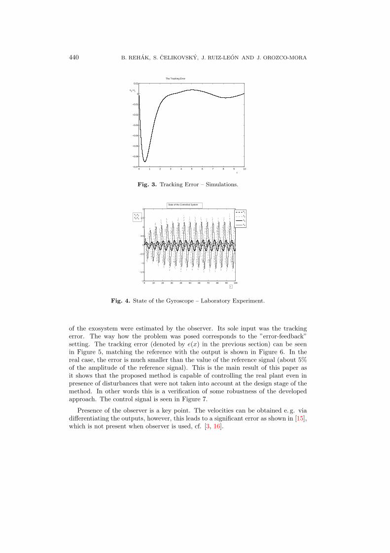
440 B. REHAK, S. CELIKOVSKY, J. RUIZ-LEON AND J. OROZCO-MORA
0 1 2 3 4 5 6 7 8 9 10−0.07
−0.06
−0.05
−0.04
−0.03
−0.02
−0.01
0
0.01
The Tracking Error
x3−v
1
t
Fig. 3. Tracking Error – Simulations.
0 10 20 30 40 50 60 70 80 90 100−2
−1.5
−1
−0.5
0
0.5
1
1.5
2
x
1
x2
x3
x4
State of the Controlled System
x1,x
2x
3,x
4
t
Fig. 4. State of the Gyroscope – Laboratory Experiment.
of the exosystem were estimated by the observer. Its sole input was the trackingerror. The way how the problem was posed corresponds to the ”error-feedback”setting. The tracking error (denoted by e(x) in the previous section) can be seenin Figure 5, matching the reference with the output is shown in Figure 6. In thereal case, the error is much smaller than the value of the reference signal (about 5%of the amplitude of the reference signal). This is the main result of this paper asit shows that the proposed method is capable of controlling the real plant even inpresence of disturbances that were not taken into account at the design stage of themethod. In other words this is a verification of some robustness of the developedapproach. The control signal is seen in Figure 7.
Presence of the observer is a key point. The velocities can be obtained e. g. viadifferentiating the outputs, however, this leads to a significant error as shown in [15],which is not present when observer is used, cf. [3, 16].

Methods for the Solution of the Nonlinear Output Regulation Problem 441
0 10 20 30 40 50 60 70 80 90 100−0.2
−0.15
−0.1
−0.05
0
0.05
0.1
0.15
Tracking Error
x3−w
1
t
Fig. 5. Tracking Error – Laboratory Experiment.
0 10 20 30 40 50 60 70 80 90 100−0.4
−0.3
−0.2
−0.1
0
0.1
0.2
0.3
0.4
x
3
w1
Output and Reference
w1,x
3
t
Fig. 6. Output and Reference – Laboratory Experiment.
0 10 20 30 40 50 60 70 80 90 100−1
−0.8
−0.6
−0.4
−0.2
0
0.2
0.4Control Signal
u(t)
t
Fig. 7. Control – Laboratory Experiment.
442 B. REHAK, S. CELIKOVSKY, J. RUIZ-LEON AND J. OROZCO-MORA
7. IMPLEMENTATION ASPECTS AND METHODS COMPARISON
The systems of partial differential equations were solved using the software packageFEMLAB 2.3. (Today, its successor is called Comsol Multiphysics). It is a powerfulsolver that easily enables to define the problem. Moreover, even the peculiar featuresof the regulator equation (first order, no boundary conditions) could be handled. Themesh on which the problem was solved was generated by the Femlab’s built-in meshgenerator. In order to guarantee the condition xi = 0, the mesh was refined in theneighborhood of the origin.
Femlab offers its own postprocessing functions to use the solution further. Theywere used to obtain simulations. This was necessary as this set of functions includesan interpolation function or computation of the integral defining the error functional.However, to use the results without Femlab, the results were interpolated on thenodes of a pre-defined grid (which may be different from the grid used for evaluationof the solution) so that standard Matlab interpolation can be used.
Both the newly developed methods proved to be viable for practical implementa-tion. They possess some features that are common to them but they differ in someothers. The main difference is the speed of computations. The method based on theminimization of the error functional requires a successive evaluation of the regulatorequation. Moreover, the optimization method also involves some extra expenses.The method based on singular-perturbation does not suffer from this drawback asthe solution of the equation (9) is evaluated once. On the other hand, the variablec is a part of the solution which implies higher demand for memory. This mightbe an issue if a fine mesh is required. A problem is also a not fully investigatedconvergence of this method. However, as in practice one has to solve the perturbedequation only, the Theorem gives a useful condition guaranteeing existence of solu-tion of the perturbed regulator equation.
The estimate of the tracking error when using the feedforward based on thenumerical approximation of the solution of the regulator equation is contained in[17]. Even if this article deals with the optimization-based method only, the estimateis applicable for the singular perturbation-based one as well as evaluating the errorfunctional for the solution of (9) can be carried out analogously in this case. Theeffect of the discretization of the equations solved by the FEM solver is discussedin the cited article as well, this analysis is also valid for both methods. A featurethat deserves a special note here is the high tolerance to coarse discretization of thedomain Ωb.
8. CONCLUSION
Several methods to solve the regulator equation arising in the output regulationproblem were presented and discussed. The detailed mathematical analysis of oneof them was performed, namely, of the singular perturbation based method. Furtherimplementation aspects of this method are discussed and compared to other knownpresented methods. Finally, the singular perturbation method was also tested onlaboratory system via experiment on a laboratory gyroscopical system to show thatit can be potentially applicable for real-time control design.

Methods for the Solution of the Nonlinear Output Regulation Problem 443
ACKNOWLEDGEMENT
This work was partially supported by the Czech Science Foundation through the grantsNos. 102/07/P413 and 102/08/0186 and by the National Council of Science and Technologyof Mexico (CONACyT).
(Received August 14, 2007.)
REFERENCES
[1] C. I. Byrnes, F. Delli Priscoli, A. Isidori, and W. Kang: Structurally stable outputregulation of nonlinear systems. Automatica 33 (1997), 369–285.
[2] S. Celikovsky and B. Rehak: Output regulation problem with nonhyperbolic zerodynamics: a FEMLAB-based approach. In: Proc. 2nd IFAC Symposium on System,Structure and Control 2004, Oaxaca 2004, pp. 700–705.
[3] S. Celikovsky and B. Rehak: FEMLAB-based error feedback design for the outputregulation problem. In: Proc. Asian Control Conference 2006. Bandung 2006.
[4] S. Devasia: Nonlinear inversion-based output tracking. IEEE Trans. Automat. Con-trol 41 (1996), 930–942.
[5] B.A. Francis and W.M. Wonham: The internal model principle of control theory.Automatica 12 (1976), 457–465.
[6] B.A. Francis: The linear multivariable regulator problem. SIAM J. Control Optim.15 (1977), 486–505.
[7] J. S.A. Hepburn and W.M. Wonham: Error feedback and internal models on differ-entiable manifolds. IEEE Trans. Automat. Control 29 (1981), 397–403.
[8] J. Huang: Nonlinear Output Regulation: Theory and Applications. SIAM, New York2004.
[9] J. Huang: Output regulation of nonlinear systems with nonhyperbolic zero dynamics.IEEE Trans. Automat. Control 40 (1995), 1497–1500.
[10] J. Huang: On the solvability of the regulator equations for a class of nonlinear sys-tems. IEEE Trans. Automat. Control 48 (2003), 880–885.
[11] J. Huang and W. J. Rugh: On a nonlinear multivariable servomechanism problem.Automatica 26 (1990), 963–972.
[12] A. Isidori and C. I. Byrnes: Output regulation of nonlinear systems. IEEE Trans.Automat. Control 35 (1990), 131–140.
[13] A. Isidori: Nonlinear Control Systems. Third edition. Springer, Berlin –Heidelberg –New York 1995.
[14] H.K. Khalil: Nonlinear Systems. Pearson Education Inc., Upper Saddle River 2000.
[15] B. Rehak, J. Orozco-Mora, S. Celikovsky, and J. Ruiz-Leon: FEMLAB-based outputregulation of nonhyperbolically nonminimum phase system and its real-time imple-mentation. In: Proc. 16th IFAC World Congress, Prague, IFAC 2005.
[16] B. Rehak, J. Orozco-Mora, S. Celikovsky, and J. Ruiz-Leon: Real-time error-feedbackoutput regulation of nonhyperbolically nonminimum phase system. In: Proc. Amer-ican Control Conference 2007, New York 2007.
444 B. REHAK, S. CELIKOVSKY, J. RUIZ-LEON AND J. OROZCO-MORA
[17] B. Rehak and S. Celikovsky: Numerical method for the solution of the regulatorequation with application to nonlinear tracking. Automatica 44 (2008), 1358–1365.
[18] H.-G. Roos, M. Stynes, and L. Tobiska: Numerical Methods for Singularly PerturbedDifferential Equations. Springer, Berlin 1996.
[19] J. Ruiz-Leon, J. L. Orozco-Mora, and D. Henrion: Real-time H2 and H∞ controlof a gyroscope using Polynomial Toolbox 2.5. In: Latin-American Conference onAutomatic Control CLCA 2002, Guadalajara 2002.
[20] A.B. Vasil’eva and B. F. Butuzov: Asymptotic Expansions of Solutions of SingularlyPerturbed Equations (in Russian). Nauka, Moscow 1973.
Sergej Celikovsky and Branislav Rehak, Institute of Information Theory and Automation
– Academy of Sciences of the Czech Republic, Pod Vodarenskou vezı 4, 182 08 Praha 8.
Czech Republic.
e-mails: [email protected], [email protected]
Javier Ruiz-Leon, CINVESTAV-IPN, Avenida Cientıfica 1145, Col. El Bajıo, 45015 Za-
popan, Jalisco. Mexico.
e-mail: [email protected]
Jorge Orozco-Mora, Instituto Tecnologico de Aguascalientes, Av. Tecnologico No. 1801
Ote. Fracc. Bona Gens, C.P. 20256, Aguascalientes, Ags. Mexico.
e-mail: [email protected]


![Generalized expectation with general kernels on g ...library.utia.cas.cz/separaty/2017/E/mesiar-0477104.pdfIn Markov diffusion process, Lerner [15] proved a Jensen’s inequality for](https://static.fdocuments.net/doc/165x107/5f0397777e708231d409cf59/generalized-expectation-with-general-kernels-on-g-in-markov-diffusion-process.jpg)


