������������������ �������������������������������� ����������������������� �������

Understanding Frequency Modulation (FM), Frequency Shift Keying (FSK), Sunde’s FSK and MSK andsome more

The process of modulation consists of mapping the information on to an electromagnetic medium (acarrier). This mapping can be digital or it can be analog. The modulation takes place by varying the threeparameters of the sinusoid carrier.

1. Map the info into amplitude changes of the carrier2. Map the info into changes in the phase of the carrier3. Map the info into changes in the frequency of the carrier.

The first method is known as amplitude modulation. The second and third are both a from of anglemodulation, with second known as phase and third as frequency modulation.

Let’s start with a sinusoid carrier given by its general equation

0( ) cos(2 )c cc t A f tπ φ= +

This wave has an amplitude Ac a starting phase of fð

0 and the carrier frequency, f

c. The carrier in Figure

1 has amplitude of 1 v, with fc of 4 Hz and starting phase of 45 degrees.

Generally when we refer to amplitude, we are talking about the maximum amplitude, but amplitude alsomeans any instantaneous amplitude at any time t, and so it is really a variable quantity depending on where youspecify it.

Figure 1 – A sinusoid carrier of frequency 4, starting phase of 45 degrees and amplitude of 1 volt.

The amplitude modulation changes the amplitude (instantaneous and maximum) in response to theinformation. Take the following two signals; one is analog and the other digital

.

a. Analog message signal, m(t)

b. Binary message signal, m(t)

Fig 2 – Two arbitrary message signals, m(t)

About Amplitude Modulation (AM)

The amplitude modulated wave is created by multiplying the amplitude of a sinusoid carrier with themessage signal.

( ) ( ) ( )s t m t c t=

0cos(2 )( )c cA m t f tπ φ= +

The modulated signal shown in Figure 3, is of carrier frequency fc but now the amplitude changes in

response to the information. We can see the analog information signal as the envelope of the modulated signal.Same is true for the digital signal.

a. Amplitude modulated carrier shown with analog message signal as its envelope

c. Amplitude modulated carrier shown with binary message signal as its envelope

Figure 3 – Amplitude modulated carrier, a. analog, b. digital

Let’s look at the argument of the carrier. What is it?

The argument is an angle in radians. The argument of a cosine function is always an angle we know thatfrom our first class in trigonometry. The second term is what is generally called the phase. In amplitudemodulation only the amplitude of the carrier changes as we can see above for both binary and analog messages.Phase and frequency retain their initial values.

Any modulation method that changes the angle instead of the amplitude is called angle modulation. Theangle consists of two parts, the phase and the frequency part. The modulation that changes the phase part iscalled phase modulation (PM) and one that changes the frequency part is called frequency modulation (FM).

How do you define frequency? Frequency is the number of 2 pð revolutions over a certain time period.Mathematically, we can write the expression for average frequency as

( ) ( )

2i i

t

t t tf

t

φ φπ∆

+ ∆ −=∆ 1

This equation says; the average frequency is equal to the difference in the phase at time t + Dðt andtime t, divided by 2pð (or 360 degrees if we are dealing in Hz.)

Example: a signal changes phase from 45 to 2700 degrees over 0.1 second. What is its average fre-quency?

2700 45

360*0.1

−= = 73.75 Hz

This is the average frequency over time period t = 0.1 secs. Perhaps it will be different over 0.2 secs orsome other time period or maybe not, we don’t know.

What is the instantaneous frequency of this signal at any particular moment in the 0.1 second period? Wedon’t really know given this information.

The instantaneous frequency is defined as the limit of the average frequency as Dðt gets smaller andsmaller and approaches 0. So we take limit of equation 1 to create an expression for instantaneous frequency,f

i(t),.

The fi(t) is the limit of f

Dðt(t) as Dðt goes to 0. The phase change over time Dðt is changed to a differential

to indicate change from discrete to continuous.

0

0

( ) lim ( )

( ) ( )lim

2

( )1

2

i tt

i i

t

i

f t f t

t t t

t

d t

dt

φ φπ

φπ

∆∆ →

∆ →

=

+ ∆ −=∆

=

This last result is very important in developing understanding of both phase and frequency modulation!The 2pð factor has been moved up front. The remaining is just the differential of the phase.

Another way we can state this is by recognizing that radial frequency wð is equal to

2 ( )if tω π=

It is also equal to the rate of change of phase,

( ( ))id t

dt

φω =

so again we get,

( )1( )

2i

t

d tf t

dt

φπ

= 2

Intuitively, it says; the frequency of a signal is equal to its phase change over time. When seen as aphasor, the signal phasor rotates in response to phase change. The faster it spins (phase change), the higher itsfrequency.

What does it mean, if I say: the phasor rotates for one cycle and then changes directions, goes the oppo-

site way for one cycle and then changes direction again? This is a representation of a phase modulation.Changing directions means the signal has changed its phase by 180 deg.

We can do a simple minded phase modulation this way. Go N spins in clockwise directions in response toa 1 and N spins in counterclockwise directions in response to a 0. Here N represents frequency of the phasor.

Figure 4 – The carrier as a phasor, the faster it spins, the higher the frequency.

If frequency is the rate of change of phase, then what is phase in terms of frequency? As we know fromdefinition of frequency that it is number of full 2 pð rotations in a time period.

Given, a signal has traveled for 0.3 seconds, at a frequency of 10 Hz with a starting phase of 0, what isits phase now?

2 10 2 .3 20iPhase now f t Hz radiansφ π π= = × × =

This is an integration of the total number of radians covered by the signal in 0.3 secs. Now we write thisas an integral,

.3

0( ) 2 ( )i it f t dtφ π= ∫

and since this is average frequency, it is constant over this time period, we get

2 10 2 .3 20iPhase now f t Hz radiansφ π π= = × × =

We note the phase and frequency are related by

Phase a Integral of frequency

Frequency a Differential of phase

Phase modulation

Let the phase be variable. Going back to the original equation of the carrier, change the phase (theunderlined term only) from a constant to a function of time.

2 () ))( cos(c cc tA tt fπ φ= + 3

We can phase modulate this carrier by changing the phase in response to the message signal.

( ) ( )i pt k m tφ =

Now we can write the equation for the carrier with a changing phase as

( ) cos(2 ( ))c pcs t A f kt m tπ= + 4

The factor pk is called the phase sensitivity factor or the modulation index of the message signal. For

analog modulation, this expression is called the phase modulation. In phasor representation of an analog PM,the phasor slows down gradually to full stop and then again picking up speed in the opposite direction gradu-ally.

In binary case, the phasor does not slow down gradually but stops abruptly. This is easy to imagine. Takea look at equation 4. Replace the underlined terms by a 0 or a 1, or better yet, replace it by 180oð if m(t) is 1and -180oð if it is a 0. Now, we have a binary PSK signal. The phase changes from -180oð to +180o in re-sponse to a message bit.

This is the main difference between analog and digital phase modulation in that in digital, the phasechanges are discrete and in analog, they are gradual and not obvious. For binary PSK, phase change is mappedvery simply as two discrete values of phase.

( ) cos(2 )c c js t a f tπ φ= + 0j orφ π=

a. Phase modulation is response to a binary message. The phase changes are abrupt.

b. Phase modulation is response to an analog message. The phase changes are smooth.

Figure 5 – Phase modulated carrier for both binary and analog messages.

Frequency modulation

FM is a variation of angle modulation where instead of phase, we change the frequency of the carrier inresponse to the message signal.

Vary the frequency by adding a time varying component to the carrier frequency.

( ) ( )t c ff t f k m t= +

where fc is the frequency of the unmodulated carrier, and k

f a scaling factor, and m(t), the message signal.

The term kf m(t) can called a deviation from the carrier frequency.

Example, a carrier with fc = 100, k

f = 8 and message bit rate = 1. Assume the message signal is polar so

we have 1 for a 1 and -1 for 0.

For m(t) = 1, we get

1f = 100+ 8(1) = 108 Hz

for m(t) = -1

2f = 100- 8(1) = 92 Hz

The phasor rotates at a frequency of 108 Hz, as long as it has a signal of 1 and at 92 Hz for a signalindicating a 0 bit.

Remember the equation relating phase and frequency

( )1( )

2i

i

d tf t

dt

θπ

= 5

which can also be written as

( ) 2 ( )t

i it f t dtφ π−∞

= ∫ 6

Now look at the carrier equation,

( ) cos(2 )c c is t A f tπ φ= + 7

We define the instantaneous frequency of this signal as the sum of a constant part, which is the carrierfrequency, and a changing part as show below.

( ) ( )t c ff t f k m t= + 8

The argument of the carrier is an angle. So we need to convert this frequency term to an angle. Do that by

taking the integral of this expression (invoke equation 6)

( ) 2 2 ( )t t

i c ft f dt k m t dtθ π π−∞ −∞

= +∫ ∫

and since fc is a constant, this is just equal to

( ) 2 2 ( )t

i c ft f t k m t dtθ π π−∞

= + ∫ 9

Now we plug this as the argument of the carrier into equation 7 and we get

( ) cos (2 2 ( ) )t

c c fs t A f t k m t dtπ π−∞

= + ∫ 10

This represent the equation of a FM modulated signal. A decidedly unpleasant looking equation! This isabout as far as you can get from intuitive. There is no resemblance at all to anything we can imagine.

Analog FM is one of the more complex ideas in communications. It is very difficult to develop an intuitivefeeling for it. Bessel functions rear their multi-heads here and things go from bad to worse. Thankfully this iswhere binary signals come to the rescue. The binary or digital form of Frequency Modulation is very easy tounderstand .

But before we do that, examine the following relationship between FM and PM.

Let’s write out both equations side by side so we can see what’s going on.

PM: ( ) cos(2 ( ))c pcs t A f kt m tπ= + 11

FM: ( ) cos (2 2 ( ) )t

c c fs t A f t k m t dtπ π−∞

= + ∫ 12

Note that in FM, we integrate the message signal before modulating. Both FM and PM modulated signalsare conceptually identical, the only difference being in the first case phase is modulated directly by the messagesignal and in FM case, the message signal is first integrated and then used in place of the phase.

Using a Phase modulator we can create a FM signal by just integrating the message signal first. Similarlywith a FM modulator we can create a PM signal by differentiating the message signal before modulation.

Differentiator

FrequencyModulator

Integrator

PhaseModulator

m(t)

Derivativeof m(t)

Integralof m(t)

A FM signal

A PM signal

Figure 6 – Phase and Frequency modulators are interchangeable by just changing the form of the message signal.Differentiate the message signal and then feed to a PM modulator to get a FM signal and vice-versa for FM.

Frequency Shift Keying – the digital form of FM

The binary version of FM is called the Frequency Shift Keying or FSK. Here the frequency does not keepchanging gradually over symbol time but changes in discrete amounts in response to a message similar tobinary PSK where phase change is discrete.

The modulated signal can be written very simply as consisting of two different carriers.

1 1

2 2

( ) cos(2 )

( ) cos(2 )c

c

s t A f t

s t A f t

ππ

==

s1(t) in response to a 1 and s

2(t) in response to a 0.

Getting sophisticated, this can be written as a deviation from the carrier frequency.

1

2

( ) cos(2 ( ) )

( ) cos(2 ( ) )c c

c c

s t A f f t

s t A f f t

ππ

= − ∆= + ∆

Here Dðf is called the frequency deviation. This is excursion of the signal above and below the carrierfrequency and indicates the quality of the signal such in stereo FM reception.

Each of these two frequencies f1 and f

2, are an offset from the carrier frequency, f

c. Let’s call the higher of

these fh and lower f

l,. Now we can create a very simple FM modulator as shown the Figure 7. We can use this

table to modulate the incoming message signal.

Amplitude ofm(t) f

h f

l

-1 0 1+1 1 0

We send fl in response to a -1 and 0 in response to a +1. When we get a change from a -1 to +1, we

switch frequency, so that only one signal, either fh or fl is transmitted.

The combined signal can be written as, keeping mind that two terms are orthogonal in time and neveroccur at the same time.

( ) cos(2 ) cos(2 )BFSK h h h l l ls t A f t A f tπ φ π φ= + + + 13

Figure 7 – A FSK modulator

In the modulator shown here, we are changing the amplitude Al and A

h which are either 0 or 1 in response

to the message signal, but never present at the same time.

The above process looks very much like amplitude modulation. The only difference is that the signalpolarity goes from 0 to 1(because A

h is either 0 or 1), rather than -1 to +1 as it does in BPSK. This is an

important difference and we can try to understand FM better by making this clever substitution (Ref. 1).

'

'

1 1( ) ( )

2 21 1

( ) ( )2 2

h h

l l

A t A t

A t A t

= +

= +14

These transformations turn Ah and A

l from 0,1 to -1, +1.

Now we substitute these into equation 13 and get,

' '

( ) cos(2 ) cos(2 )

cos(2 ) cos(2 )

BFSK h h l l

h h h l l l

s t f t f t

A f t A f t

π φ π φ

π φ π φ

= + + +

+ + + + 15

The first two terms are just cosines of frequencies fh and f

l, so their spectrum contribution is an impulse at

frequencies fh and f

l. The second two terms are amplitude modulated carriers. These last two terms give rise to

a sin x/x type of spectrum of the square pulse as shown below.

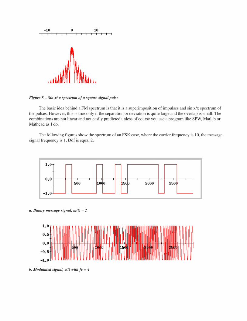
Figure 8 – Sin x/ x spectrum of a square signal pulse

The basic idea behind a FM spectrum is that it is a superimposition of impulses and sin x/x spectrum ofthe pulses. However, this is true only if the separation or deviation is quite large and the overlap is small. Thecombinations are not linear and not easily predicted unless of course you use a program like SPW, Matlab orMathcad as I do.

The following figures show the spectrum of an FSK case, where the carrier frequency is 10, the messagesignal frequency is 1, Dðf is equal 2.

a. Binary message signal, m(t) = 2

b. Modulated signal, s(t) with fc = 4

Figure 9- Spectrum of the modulated signal, Dðf is equal 2. Note the two impulses at frequencies 2 and 6 Hz.

Here we see clearly that there are two impulses representing the carrier frequencies, 2 and 6. If youignore, these, the remaining are just two sin x/ x spectrums centered at frequencies 2 and 6, added together.

We define a term called the modulation index of a FM signal.

m

fm

f

∆= 16

where Dðf is what is called the frequency deviation, and fm is the frequency of the message signal.

2 1

2

f ff

−∆ =

This factor m, determines the occupied bandwidth and is a measure of the bandwidth of the signal.

The FM broadcasting in the US takes place at carrier frequencies of app. 50 MHz. The message signalwhich is music, has frequency content up to about 15 kHz. The FCC allows deviation of 75 kHz. For this, them is

7515

5m

fm

f

∆= = =

m, is independent of the carrier frequency and depends only on the message signal frequency and theallowed deviation frequency. This factor is not constant for a particular signal as is the AM modulation index.In FM broadcasting m can go very high, since the message signal has some pretty low frequencies, such as 50Hz. For FM it can vary any where from 1500 to 5 on the low end.

FM signal is classified in two categories,

Signals with m << 1 are called Narrowband FM

Signals with m >> 1 are called Wideband FM

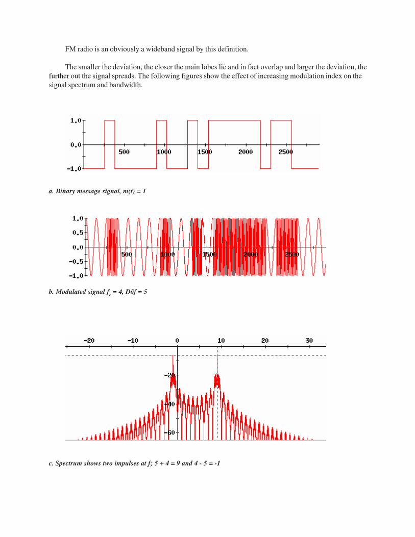
FM radio is an obviously a wideband signal by this definition.

The smaller the deviation, the closer the main lobes lie and in fact overlap and larger the deviation, thefurther out the signal spreads. The following figures show the effect of increasing modulation index on thesignal spectrum and bandwidth.

a. Binary message signal, m(t) = 1

b. Modulated signal fc = 4, Dðf = 5

c. Spectrum shows two impulses at f; 5 + 4 = 9 and 4 - 5 = -1

d. Modulated signal, fc = 4, Dðf = 10

e. Spectrum shows two impulses at f; 10 + 4 = 14 and 4-10 = -6Note that the spectrum does look like a superposition of impulses and sinc functions.

f. Modulated signal, fc = 4, Dðf = 1

g. Spectrum shows two impulses at f; 1 + 4 = 5 and 4 - 1 = 3

h. Modulated signal, fc = 4, Dðf = .4

i. Spectrum shows two impulses at f; 4 + .1 = 4.1 and 4 - .11 = 3.9

Figure 10 – Relationship of FM modulation index and its spectrum. As index gets large, the signal bandwidthincreases. In these figures, we can define the bandwidth as the space between the main lobes or impulses.

In fact as kf gets very small, the general rules of identifying the impulses do not apply and we have to

know about Bessel functions in order to compute the spectrum.

There are two very special cases of FM that bear discussing.

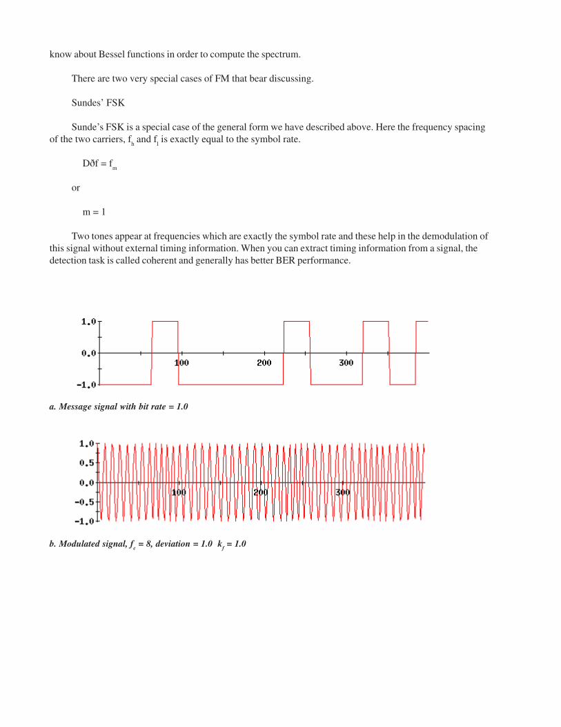
Sundes’ FSK

Sunde’s FSK is a special case of the general form we have described above. Here the frequency spacingof the two carriers, f

h and f

l is exactly equal to the symbol rate.

Dðf = fm

or

m = 1

Two tones appear at frequencies which are exactly the symbol rate and these help in the demodulation ofthis signal without external timing information. When you can extract timing information from a signal, thedetection task is called coherent and generally has better BER performance.

a. Message signal with bit rate = 1.0

b. Modulated signal, fc = 8, deviation = 1.0 k

f = 1.0

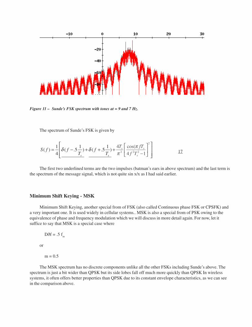
Figure 11 – Sunde’s FSK spectrum with tones at = 9 and 7 Hz.

The spectrum of Sunde’s FSK is given by

2

2 2 2

1 1 1( ) ( .5 ) ( .5 )

4

4 cos(

4 1s s

s s s

T fT

fS f f f

T T T

ππ

δ δ −

= − + + +

17

The first two underlined terms are the two impulses (batman’s ears in above spectrum) and the last term isthe spectrum of the message signal, which is not quite sin x/x as I had said earlier.

Minimum Shift Keying - MSK

Minimum Shift Keying, another special from of FSK (also called Continuous phase FSK or CPSFK) anda very important one. It is used widely in cellular systems.. MSK is also a special from of PSK owing to theequivalence of phase and frequency modulation which we will discuss in more detail again. For now, let itsuffice to say that MSK is a special case where

Dðf = .5 fm

or

m = 0.5

The MSK spectrum has no discrete components unlike all the other FSKs including Sunde’s above. Thespectrum is just a bit wider than QPSK but its side lobes fall off much more quickly than QPSK In wirelesssystems, it often offers better properties than QPSK due to its constant envelope characteristics, as we can seein the comparison above.

a. MSK modulated signal, m(t) = 2.0, Dðf = 1

MSK spectrums does look a lot like a QPSK spectrum but is not the same.

Figure 12 – MSK signal and spectrum. Note that it has no “Batman ears” as in all other FSKs.

The spectrum of MSK is given by

2

2 2 2

16 cos(

1(

1)

2

6s s

s

T fT

fS f

T

ππ

−

=

18

(We will discuss MSK again from PSK point of view in the next tutorial.)

M-ary FSK

A M-ary FSK is just an extension of BFSK. Instead of two carriers, we have M. These carriers can beorthogonal or not, but the orthogonal case would obviously give better BER.

M-ary FSK requires considerably larger bandwidth than M-PSK but as M increases, the BER goes downunlike M-PSK. Infact if number of frequencies are increased, M-FSK becomes an OFDM like modulation.

Analog FM

Response to a sinusoid – not as simple as we would like

I have side-skirted the issue of analog FM’s complicated spectrum. Binary or digital FSK allows us todelve into FM and is easy to understand but a majority of FM transmission such for radio is analog. So we willtouch on that aspect to give you the full understanding.

Now we will look at what happens to a message signal that is a single sinusoid of frequency fm

when it isFM modulated.

( ) cos (2 2 ( ) )t

c c fs t A f t k m t dtπ π−∞

= + ∫ 19

Let’s take a message signal as shown below.

Figure 13 – Just a lowly sinusoid that is about to be mangled to high-fidelity heights by a FM modulator.

( ) cos(2 2 sin )mc c fs t A f t k f tπ π= +

Now set Ac = 1 and switch to radial frequency for convenience ( less typing.)

( ) cos( sin )c f ms t t k tω ω= +

By the well-known trigonometric relationship, this equation is becomes

( ) cos( sin )

cos cos( sin ) sin sin( sin )c f m

c f m c f m

s t t k t

t k t t k t

ω ωω ω ω ω

= +

= − 20

Now the terms cos( sin )f mk tω can be expanded. How and why, we leave it to the mathematicians, and

see that we again get a pretty hairy looking result.

0 2 4cos( sin ) ( ) 2 ( )cos(2 ) 2 ( )cos(4f m f f m fk t J k J k t J kω ω ω= + + 21

The sin( sin )f mk tω is similarly written as

1 3 5sin( sin ) 2 ( )sin( ) 2 ( )sin(3 ) 2 (f m f m f mk t J k t J k t J kω ω ω= + +

22

(Note kf = m)

The underlined functions are Bessell functions and are function of the modulation index m or kf. They are

seen many places where harmonic signals analysis and despite my bad-mouthing, they are quite harmless andbenign. There are just so many of them. They ones here are of first kind and of order n. The terms of the cosineexpansion since it is an even function, contain only even harmonics of w

m and sin expansion has only odd

harmonics and this is obvious if you will examine the above equations even casually.

Figure 14 shows the general shape of 4 Bessel functions as the order is increased. The x-axis is modula-tion index k

f and the y-axis is the value of the Bessel function value. For example, for k

f = 2, the values of the

various Bessel functions are

J0 = .25J1 = .65J2 = .25J3 = .18

The FM carriers take their amplitude values from these functions as we will see below.

Figure 14 – Bessel function of the first kind of order n, shown for order = 0, 1, 2 and 4X-axis is read as the modulation index k

f, and y-axis is the value of the amplitude of the associated harmonic.

Except for the 0 – order function, all others start at 0.0 and damp down with cycle.

Below we see a plot of what the cos and sin expansions (equations 22, 21) containing the various Besselfunctions look like for just four terms.

0 0.2 0.4 0.61.5

1

0.5

0

0.5

10.96

1.028

expfcos 5 t,( )

0 t

Figure 15 – Plot of 0 2 4cos( sin ) ( ) 2 ( ) cos(2 ) 2 ( )cos(4f m f f m fk t J k J k t J kω ω ω= + +

0 0.2 0.4 0.62

1

0

1

21.085

1.085

expfsin 5 t,( )

0 t

Figure 16 – Plot of 1 3 5sin( sin ) 2 ( )sin( ) 2 ( )sin(3 ) 2 (f m f m f mk t J k t J k t J kω ω ω= + +

Now we put it all together (plug equations 21, 22 into equation 20)And by trigonometric magic get, an expression for the FM modulated signal.

[ ][ ][ ]

0

1

2

3

( ) ( ) cos( )

( ) cos( ) cos( )

( ) cos( 2 ) cos( 2 )

( ) cos( 3 ) cos( 3 )

...

f c

f c m c m

f c m c m

f c m c m

s t J k t

J k t t

J k t t

J k t t

ω

ω ω ω ω

ω ω ω ω

ω ω ω ω

=

− − − +

+ − − +

− − − +

+

Remember this is a response to just one single solitary sinusoid. This signal contains the carrier with

amplitude set by Bessel function of 0 order (the first underlined term), and sideband on each side of the carrier

at harmonically related separations of , 2 , 3 , 4 ,...m m m mω ω ω ω . This is very different from AM, in that we

know that in AM, a single sinusoid would give rise to just two sidebands (FFT of the sinusoid) on each side ofthe carrier. So many sidebands, in fact an infinite number of them, for just one sinusoid!

Each of these components has a Bessel function as its amplitude value. For certain values of kf, we can

see that J0 function can be 0. In such case there would no carrier at all (MSK) and all power is in sidebands.For the case of k

f = 0, which also means that there is no modulation, all power is in the carrier and all sideband

Bessel function values are zero.

FM is called a constant envelope modulation. As we know the power of a signal is function of its ampli-tude only. We note that the total power of the signal is constant and not a function of the frequency. For FM,the power gets distributed amongst the sidebands, the total power always remains equal to the square of theamplitude and is constant..

Here we plot the above signal for kf = 2 and k

f = 1.

Figure 17 – Modulated FM signal for kf = 2 and k

f = 1, the red signal is moving faster indicated higher frequency

components .

Examples of FM spectrums to a sinusoid.

In the following signals, the only thing we are changing is the modulation index kf. This increases the

frequency separation (or deviation and increases the bandwidth.)

kf = 0.5

kf = 1

kf = 2

kf = 4

Figure 18 – Time domain FM signals for various kf values.

Figure 19 – Spectrum of FM signals for various kf values.

Bandwidth of a FM signal

The bandwidth of an FM signal is kind of slippery thing. Carson’s rule states that is bandwidth of a FMsignal is equal to

. 2( )est mBandwidth f f= ∆ +

Here

2m

s

fT

=

or is equal to the baseband symbol rate, Rs.

If the frequencies f1 and f2 chosen satisfy the following equation, the cross-correlation between thecarriers is zero, then this is an orthogonal set.

0

1 2

0

cos(2 )cos(2 ) 0T

f t f t dtρ π π= =∫

The output of I is maximum just when output of Q channel is zero. The decision at the receiver is asimple matter of determining if the voltage is present.

The BER of a BFSK system is given by

2

0

1 11

2 2s

e

EP erf

N

= −

If however, if the cross-correlation is not zero,

0

1 2

0

cos(2 )cos(2 ) 0T

f t f t dtρ π π= ≠∫

then energy is present on both channels at the same time and in presence of noise, symbol decision may beflawed. Expanding above equation, we get,

2 1 2 1

2 1

sin( ( ) ) cos( ( ) )

( )s s

s

f f T f f T

f f T

π πρπ

− −=−

Now set

2 1

4( ) 4s f

m

ff f T k

f

∆− = =

sin(4 ) cos(4 )

4f f

f

k k

k

π πρ

π=

Figure 20 – Cross-correlation between I and Q FSK signals. The zero crossing points are the preferable points ofoperation.

Plotting this equation against the 2 times modulation index kf, we get Figure 20. The y-axis which is

correlation between I and Q channels is 0 at specific values of kf. These values are 1, 2, 3 and 4 and so on.

The point with the lowest correlation (negative value is considered the most efficient place to operate anFSK. At first zero crossing, we note that the symbols are located only half a symbol apart so, coherent detec-tion is not possible at this point. The next zero crossing, where kf = 1, is the Sunde’s FSK. Coherent detectionis possible at this point because symbols are at least ((f2-f1)Ts = 1) one symbol apart. The 4th zero crossing isMSK.

Bandwidth of Sunde’s FSK is given by

2 1

2 3( )

s s

B f f HzT T

= − + =

And for MSK,

2 1

4 5( )

s s

B f f HzT T

= − + =

Sunde’s FSK gives us the most spectrally efficient form of FSK that can be detected incoherently,whereas MSK gives us a spectrum that is a lot like QPSK but rolls-off much faster.

_______________________________________________

Questions, corrections?Please contact me,

Charan Langtonmntcastle@earthlink.netwww.complextoreal.com

Copyright Feb 2002, All rights reserved