Σ-Δ Background Subtraction and the Zipf Law

Antoine Manzanera

ENSTA - Elec. and Comp. Sc. lab32 Bd Victor, 75015 Paris, Franceantoine.manzanera@ensta.fr

http://www.ensta.fr/∼manzaner

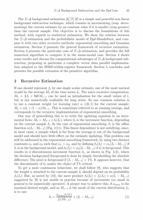
Abstract. The Σ-Δ background estimation is a simple non linear me-thod of background subtraction based on comparison and elementaryincrement/decrement. We propose here some elements of justification ofthis method with respect to statistical estimation, compared to other re-cursive methods: exponential smoothing, Gaussian estimation. We pointout the relation between the Σ-Δ estimation and a probabilistic model:the Zipf law. A new algorithm is proposed for computing the back-ground/foreground classification as the pixel-level part of a motion de-tection algorithm. Comparative results and computational advantages ofthe method are commented.

Keywords: Image processing, Motion detection, Background subtrac-tion, Σ-Δ modulation, Vector data parallelism.

1 Introduction

Background subtraction is a very popular class of methods for detecting movingobjects in a scene observed by a stationary camera [1] [2] [3] [4] [5]. In every pixelp of the image, the observed data is a time series It(p), corresponding to the val-ues taken by p in the video I, as a function of time t. As only temporal processingwill be considered in this paper, the argument p will be discarded. The princi-ple of background subtraction methods is to discriminate the pixels of movingobjects (the foreground) from those of the static scene (the background), by de-tecting samples which are significantly deviating from the statistical behaviourof the time series. To do this, one needs to estimate the graylevel distributionwith respect to time, i.e. ft(x) = P (It = x). As the conditions of the static sceneare subject to changes (lighting conditions typically), ft is not stationary, andmust be constantly re-estimated. For the sake of computational efficiency, whichis particularly critical for video processing, it is desirable that ft should be rep-resented by a small number of estimates which can be computed recursively. Inthis paper, we focus on recursive estimation of mono-modal distributions, whichmeans that we assume that the time series corresponding to the different valuespossibly taken by the background along time, presents one single mode. Thismay not be a valid assumption for every pixel, but it does not affect the interestof the principle since the technique presented can be extended to multi-modalbackground estimation.

L. Rueda, D. Mery, and J. Kittler (Eds.): CIARP 2007, LNCS 4756, pp. 42–51, 2007.c© Springer-Verlag Berlin Heidelberg 2007

Σ-Δ Background Subtraction and the Zipf Law 43

The Σ-Δ background estimation [6] [7] [8] is a simple and powerful non linearbackground subtraction technique, which consists in incrementing (resp. decre-menting) the current estimate by an constant value if it is smaller (resp greater)than the current sample. Our objective is to discuss the foundations of thismethod, with regards to statistical estimation. We show the relation betweenthe Σ-Δ estimation and the probabilistic model of Zipf-Mandelbrot, and com-pare it with two other recursive methods: exponential smoothing and Gaussianestimation. Section 2 presents the general framework of recursive estimation.Section 3 presents the particular case of Σ-Δ estimation, and provides the fullnumerical algorithm to compute it in the mono-modal case. Section 4 showssome results and discuss the computational advantages of Σ-Δ background sub-traction, proposing in particular a complete vector data parallel implementa-tion adapted to the SIMD-within-register framework. Section 5 concludes andpresents the possible extension of the primitive algorithm.

2 Recursive Estimation

If one should represent ft by one single scalar estimate, one of the most naturalwould be the average Mt of the time series It. The naive recursive computation:Mt = 1

t It + t−1t Mt−1 can be used as initialisation for the small values of t,

but is not numerically realisable for long series. So one common solution isto use a constant weight (or learning rate) α ∈]0, 1[ for the current sample:Mt = αIt + (1 − α)Mt−1. This is sometimes referred to as running average, andcorresponds to the recursive implementation of exponential smoothing.

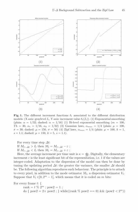
One way of generalising this is to write the updating equation in an incre-mental form: Mt = Mt−1 + δt(It), where δt is the increment function, dependingon the current sample It. In the case of exponential smoothing, δt is the affinefunction α(It −Mt−1) (Fig. 1(1)). This linear dependence is not satisfying, since,in most cases, a sample which is far from the average is out of the backgroundmodel and should have little effect on the estimate updating. This problem canstill be addressed in the exponential smoothing framework, by using two distinctconstants α1 and α2 such that α1 > α2, and by defining δt(It) = α1(It −Mt−1) ifIt is in the background model, and δt(It) = α2(It−Mt−1) if It is foreground. Thisresults in a discontinuous increment function δt, as shown in Fig. 1(2), wherethe decision background/foreground is done by simply thresholding the absolutedifference: The pixel is foreground if |It − Mt−1| > Th. It appears however, thatthe discontinuity of δt makes the choice of Th critical.

To get a more continuous behaviour, we shall follow [9], who suggests thatthe weight α attached to the current sample It should depend on its probabilityft(It). But, as noted by [10], the mere product δt(It) = ft(It) × α(It − Mt−1)suggested by [9] is not usable in practise because of increments too small ingeneral to be numerically operative. A proper way to achieve this, if αmax is themaximal desired weight, and as Mt−1 is the mode of the current distribution ft,is to use:

δt =αmaxft(It)ft(Mt−1)

× (It − Mt−1). (1)

44 A. Manzanera

If we use a Gaussian distribution as density model like in [9], we get thefollowing increment function:

δt = αmax × exp(−(It − Mt−1)2

2Vt−1) × (It − Mt−1). (2)

The model needs the temporal variance Vt. In [9], it is computed as the Gaus-sian estimation of the series (It −Mt)2. But this leads to a double auto-referencein the definitions of Mt and Vt, which is prejudicial to the adaptation capabil-ity of the algorithm. We recommend rather to compute Vt as the exponentialsmoothing of (It − Mt)2, using a fixed learning rate αV .

One of the interest of computing Vt is that it provides a natural criterion ofdecision background/foreground through the condition |It − Mt| > N ×

√Vt,

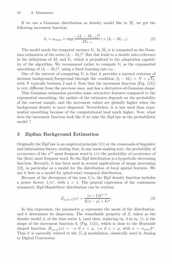
with N typically between 2 and 4. Note that the increment function (Fig. 1(3))is very different from the previous ones, and has a derivative-of-Gaussian shape.

This Gaussian estimation provides some attractive features compared to theexponential smoothing: the update of the estimates depends on the probabilityof the current sample, and the increment values are globally higher when thebackground density is more dispersed. Nevertheless, it is less used than expo-nential smoothing because of the computational load much higher. Now, whatdoes the increment function look like if we take the Zipf law as the probabilisticmodel ?

3 Zipfian Background Estimation

Originally the Zipf law is an empirical principle [11] at the crossroads of linguisticand information theory, stating that, in any sense-making text, the probability ofoccurrence of the nth most frequent word is 1/n the probability of occurrence ofthe (first) most frequent word. So the Zipf distribution is a hyperbolic decreasingfunction. Recently, it has been used in several applications of image processing[12], in particular as a model for the distribution of local spatial features. Weuse it here as a model for (pixel-wise) temporal distribution.

Because of the divergence of the sum 1/n, the Zipf density function includesa power factor: 1/ns, with s > 1. The general expression of the continuoussymmetric Zipf-Mandelbrot distribution can be written:

Z(μ,k,s)(x) =(s − 1)ks−1

2(|x − μ| + k)s. (3)

In this expression, the parameter μ represents the mode of the distribution,and k determines its dispersion. The remarkable property of Z, taken as thedensity model ft of the time series It (and then, replacing eq. 3 in eq. 1), is theshape of the increment function δt (Fig. 1(3)), which is close to the Heavisideshaped function: H(μ,κ)(x) = −κ if x < μ, +κ if x > μ, with κ = αmaxks.Thus it is naturally related to the Σ-Δ modulation, classically used in Analogto Digital Conversion:

Σ-Δ Background Subtraction and the Zipf Law 45

0 50 100 150 200 250

−8

−6

−4

−2

0

2

4

6

Affine increment function

graylevel

incr

emen

t

α=1/32

α=1/16

0 50 100 150 200 250−3

−2

−1

0

1

2

3

4

Piecewise affine increment function

graylevel

incr

emen

t

m = 100, Th=30, α1=1/16, α

2=1/32

(1) (2)

0 50 100 150 200 250

−6

−4

−2

0

2

4

6

Gaussian increment function

graylevel

incr

emen

t

μ=100,σ=30

μ=150,σ=50

0 50 100 150 200 250

−1

−0.8

−0.6

−0.4

−0.2

0

0.2

0.4

0.6

0.8

1

Zipfian increment function

graylevel

incr

emen

t

μ=100,s=1.1,k=1

μ=150,s=1.1,k=5

(3) (4)

Fig. 1. The different increment functions δt associated to the different distributionmodels: (X axis: graylevel It, Y axis: increment value δt(It)). (1) Exponential smoothing(plain: α = 1/32; dashed: α = 1/16) (1) Bi-level exponential smoothing (m = 100,Th = 30, α1 = 1/16, α2 = 1/32) (3) Gaussian laws, αmax = 1/4 (plain: μ = 100,σ = 30; dashed: μ = 150, σ = 50) (4) Zipf laws, αmax = 1/4 (plain: μ = 100, k = 1,s = 1.1; dashed: μ = 150, k = 5, s = 1.1).

For every time step Δt:If Mt−Δt > It then Mt = Mt−Δt − ε ;If Mt−Δt < It then Mt = Mt−Δt + ε ;Here, the average increment per time unit is κ = ε

Δt . Digitally, the elementaryincrement ε is the least significant bit of the representation, i.e. 1 if the values areinteger-coded. Adaptation to the dispersion of the model can then be done bytuning the updating period Δt: the greater the variance, the smaller Δt shouldbe. The following algorithm reproduces such behaviour. The principle is to attachto every pixel, in addition to the mode estimator Mt, a dispersion estimator Vt.Suppose that Vt ∈]0, 2m − 1[, which means that it is coded on m bits:

For every frame t: {rank = t % 2m ; pow2 = 1 ;do { pow2 = 2× pow2 ; } while((rank % pow2 == 0) && (pow2 < 2m))

46 A. Manzanera

If (Vt−1 > 2m

pow2) {If Mt−1 > It then Mt = Mt−1 − 1 ;If Mt−1 < It then Mt = Mt−1 + 1 ;}

Dt = |It − Mt| ;If (t % TV == 0) {

If Vt−1 > max(Vmin, N × Dt) then Vt = Vt−1 − 1 ;If Vt−1 < min(Vmax, N × Dt) then Vt = Vt−1 + 1 ;}

}

Here x%y is x modulo y. The purpose of the two first lines of the algorithm(which are computed once for all the pixels at every frame) is to find the greatestpower of two (pow2) that divides the time index modulo 2m (rank). Once thishas been determined, it is used to compute the minimal value of Vt−1 for whichthe Σ-Δ estimate Mt will be updated. Thus the (log-)period of update of Mt isinversely proportional to the (log-)dispersion: if Vt > 2m−1, Mt will be updatedevery frame, if 2m−2 ≤ Vt < 2m−1, Mt will be updated every 2 frames, andso on.

The dispersion factor Vt is computed here as the Σ-Δ estimation of the ab-solute differences Dt, amplified by a parameter N . Like in Gaussian estimation,we avoid double auto-reference by updating Vt at a fixed period TV . Vt can beused as a foreground criterion directly: the sample It is considered foreground ifDt > Vt. Vmin and Vmax are simply used to control the overflows ; 2 and 2m − 1are their typical values.

Note that the time constants, which represent the period response of thebackground estimation algorithm, are related here to the dynamics (the numberof significant bits) of Vt, and to its updating period TV . For the other methods,the time constants were associated to the inverse of the learning rates: 1/αi forthe exponential smoothing and 1/αmax and 1/αV for Gaussian estimation.

4 Results

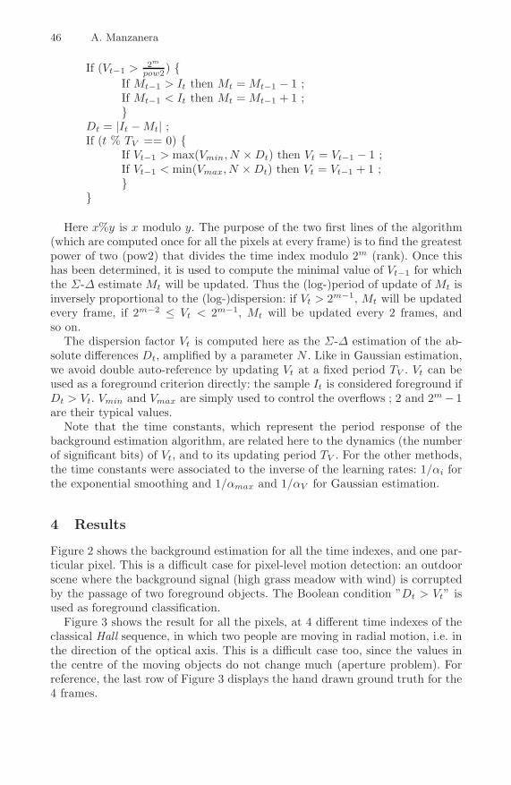
Figure 2 shows the background estimation for all the time indexes, and one par-ticular pixel. This is a difficult case for pixel-level motion detection: an outdoorscene where the background signal (high grass meadow with wind) is corruptedby the passage of two foreground objects. The Boolean condition ”Dt > Vt” isused as foreground classification.

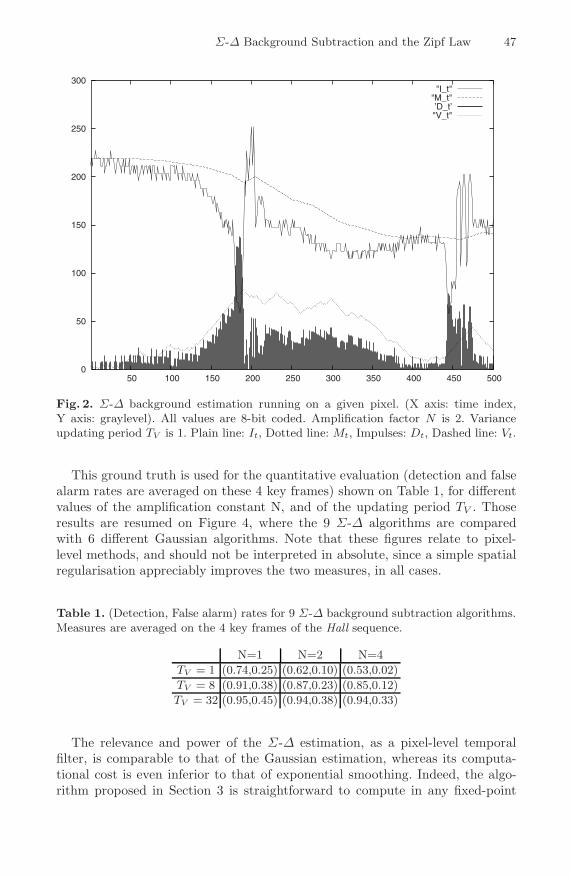
Figure 3 shows the result for all the pixels, at 4 different time indexes of theclassical Hall sequence, in which two people are moving in radial motion, i.e. inthe direction of the optical axis. This is a difficult case too, since the values inthe centre of the moving objects do not change much (aperture problem). Forreference, the last row of Figure 3 displays the hand drawn ground truth for the4 frames.

Σ-Δ Background Subtraction and the Zipf Law 47

0

50

100

150

200

250

300

50 100 150 200 250 300 350 400 450 500

"I_t""M_t"’D_t’"V_t"

Fig. 2. Σ-Δ background estimation running on a given pixel. (X axis: time index,Y axis: graylevel). All values are 8-bit coded. Amplification factor N is 2. Varianceupdating period TV is 1. Plain line: It, Dotted line: Mt, Impulses: Dt, Dashed line: Vt.

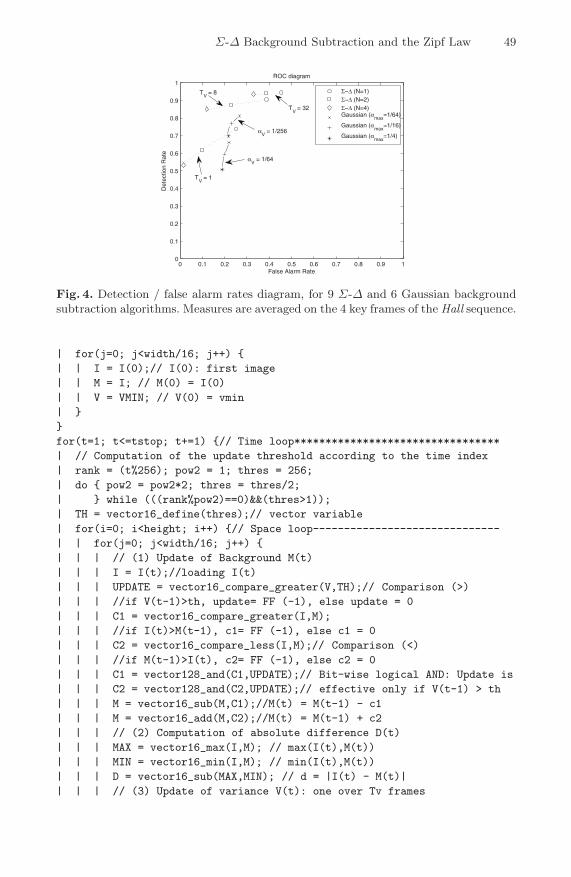
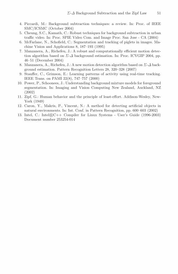
This ground truth is used for the quantitative evaluation (detection and falsealarm rates are averaged on these 4 key frames) shown on Table 1, for differentvalues of the amplification constant N, and of the updating period TV . Thoseresults are resumed on Figure 4, where the 9 Σ-Δ algorithms are comparedwith 6 different Gaussian algorithms. Note that these figures relate to pixel-level methods, and should not be interpreted in absolute, since a simple spatialregularisation appreciably improves the two measures, in all cases.

Table 1. (Detection, False alarm) rates for 9 Σ-Δ background subtraction algorithms.Measures are averaged on the 4 key frames of the Hall sequence.

N=1 N=2 N=4TV = 1 (0.74,0.25) (0.62,0.10) (0.53,0.02)TV = 8 (0.91,0.38) (0.87,0.23) (0.85,0.12)TV = 32 (0.95,0.45) (0.94,0.38) (0.94,0.33)

The relevance and power of the Σ-Δ estimation, as a pixel-level temporalfilter, is comparable to that of the Gaussian estimation, whereas its computa-tional cost is even inferior to that of exponential smoothing. Indeed, the algo-rithm proposed in Section 3 is straightforward to compute in any fixed-point

48 A. Manzanera

Fig. 3. Background subtraction shown at different frames of the Hall image sequence.Row 1: Original sequence, frames 38, 90, 170 and 250. Rows 2 and 3: Σ-Δ Backgroundand foreground, with N=2, and TV = 8. Row 4: (Fore)ground truth.

arithmetic, using an instruction set limited to: absolute difference, comparison,increment/decrement. Thus, it is well adapted to real-time implementation usingdedicated or programmable hardware.

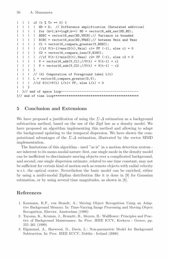
Another important computational property of Σ-Δ background subtraction,is that, once chosen the number of bits used to represent the estimates Mt andVt, every computation can be made at full precision without increasing the datawidth. This allows in particular to make the most of the data parallelism pro-vided by the SIMD-WAR (Single Instruction Multiple Data Within A Register)paradigm, which consists in concatenating many short operands in one singlevery long variable, and then applying scalar operations on the long variables.This implementation is available on most personal computers, using for exam-ple the SSE-2 (Streaming SIMD Extensions 2) instructions of the Intel R©C++compiler [13]. We provide hereunder the vectorised pseudo-code of the Σ-Δ back-ground subtraction. Here, a 16-times acceleration is achieved by performing theoperations on a 128-bit register made of 16 8-bit data.

vmin = 2; vmax = 255; logN = 1; Tv = 4;// Scalar constants definition// Vector constants definition: creates 128-bit constants// by concatenating 16 8-bit constantsVMIN = vector16_define(vmin);VMAX = vector16_define(vmax);// Sigma-Delta initializationsfor(i=0; i<height; i++) {

Σ-Δ Background Subtraction and the Zipf Law 49

0 0.1 0.2 0.3 0.4 0.5 0.6 0.7 0.8 0.9 10

0.1

0.2

0.3

0.4

0.5

0.6

0.7

0.8

0.9

1

False Alarm Rate

Det

ectio

n R

ate

ROC diagram

Σ−Δ (N=1)Σ−Δ (N=2)Σ−Δ (N=4)Gaussian (α

max=1/64)

Gaussian (αmax

=1/16)

Gaussian (αmax

=1/4)

TV = 1

αV = 1/64

αV = 1/256

TV = 8

TV = 32

Fig. 4. Detection / false alarm rates diagram, for 9 Σ-Δ and 6 Gaussian backgroundsubtraction algorithms. Measures are averaged on the 4 key frames of the Hall sequence.

| for(j=0; j<width/16; j++) {| | I = I(0);// I(0): first image| | M = I; // M(0) = I(0)| | V = VMIN; // V(0) = vmin| }}for(t=1; t<=tstop; t+=1) {// Time loop*********************************| // Computation of the update threshold according to the time index| rank = (t%256); pow2 = 1; thres = 256;| do { pow2 = pow2*2; thres = thres/2;| } while (((rank%pow2)==0)&&(thres>1));| TH = vector16_define(thres);// vector variable| for(i=0; i<height; i++) {// Space loop------------------------------| | for(j=0; j<width/16; j++) {| | | // (1) Update of Background M(t)| | | I = I(t);//loading I(t)| | | UPDATE = vector16_compare_greater(V,TH);// Comparison (>)| | | //if V(t-1)>th, update= FF (-1), else update = 0| | | C1 = vector16_compare_greater(I,M);| | | //if I(t)>M(t-1), c1= FF (-1), else c1 = 0| | | C2 = vector16_compare_less(I,M);// Comparison (<)| | | //if M(t-1)>I(t), c2= FF (-1), else c2 = 0| | | C1 = vector128_and(C1,UPDATE);// Bit-wise logical AND: Update is| | | C2 = vector128_and(C2,UPDATE);// effective only if V(t-1) > th| | | M = vector16_sub(M,C1);//M(t) = M(t-1) - c1| | | M = vector16_add(M,C2);//M(t) = M(t-1) + c2| | | // (2) Computation of absolute difference D(t)| | | MAX = vector16_max(I,M); // max(I(t),M(t))| | | MIN = vector16_min(I,M); // min(I(t),M(t))| | | D = vector16_sub(MAX,MIN); // d = |I(t) - M(t)|| | | // (3) Update of variance V(t): one over Tv frames

50 A. Manzanera

| | | if (t % Tv == 0) {| | | | ND = D; // Difference amplification (Saturated addition)| | | | for (k=1;k<=logN;k++) ND = vector16_add_sat(ND,ND);| | | | BDEC = vector16_max(ND,VMIN);// Variance is bounded| | | | BINC = vector16_min(ND,VMAX);// between Vmin and Vmax| | | | C1 = vector16_compare_greater(V,BDEC);| | | | //if V(t-1)>max(D(t),Vmin) c1= FF (-1), else c1 = 0| | | | C2 = vector16_compare_less(V,BINC);| | | | //if V(t-1)<min(D(t),Vmax) c2= FF (-1), else c2 = 0| | | | V = vector16_add(V,C1);//V(t) = V(t-1) + c1| | | | V = vector16_sub(V,C2);//V(t) = V(t-1) - c2| | | }| | | // (4) Computation of Foreground label L(t)| | | L = vector16_compare_greater(D,V);| | | //if D(t)>V(t) L(t)= FF, else L(t) = 0| | }| }// end of space loop------------------------------------------}// end of time loop**********************************************

5 Conclusion and Extensions

We have proposed a justification of using the Σ-Δ estimation as a backgroundsubtraction method, based on the use of the Zipf law as a density model. Wehave proposed an algorithm implementing this method and allowing to adaptthe background updating to the temporal dispersion. We have shown the com-putational advantages of the Σ-Δ estimation, illustrated by the vector SIMDimplementation.

The limitations of this algorithm - used ”as is” in a motion detection system -are inherent to its mono-modal nature: first, one single mode in the density modelcan be inefficient to discriminate moving objects over a complicated background,and second, one single dispersion estimate, related to one time constant, may notbe sufficient for certain kind of motion such as remote objects with radial velocityw.r.t. the optical centre. Nevertheless the basic model can be enriched, eitherby using a multi-modal Zipfian distribution like it is done in [9] for Gaussianestimation, or by using several time magnitudes, as shown in [8].

References

1. Karmann, K.P., von Brandt, A.: Moving Object Recognition Using an Adap-tive Background Memory. In: Time-Varying Image Processing and Moving ObjectRecognition, Elsevier, Amsterdam (1990)

2. Toyoma, K., Krumm, J., Brumitt, B., Meyers, B.: Wallflower: Principles and Prac-tice of Background Maintenance. In: Proc. IEEE ICCV, Kerkyra - Greece, pp.255–261 (1999)

3. Elgammal, A., Harwood, D., Davis, L.: Non-parametric Model for BackgroundSubtraction. In: Proc. IEEE ECCV, Dublin - Ireland (2000)

Σ-Δ Background Subtraction and the Zipf Law 51

4. Piccardi, M.: Background subtraction techniques: a review. In: Proc. of IEEESMC/ICSMC (October 2004)

5. Cheung, S.C., Kamath, C.: Robust techniques for background subtraction in urbantraffic video. In: Proc. SPIE Video Com. and Image Proc. San Jose - CA (2004)

6. McFarlane, N., Schofield, C.: Segmentation and tracking of piglets in images. Ma-chine Vision and Applications 8, 187–193 (1995)

7. Manzanera, A., Richefeu, J.: A robust and computationally efficient motion detec-tion algorithm based on Σ-Δ background estimation. In: Proc. ICVGIP 2004, pp.46–51 (December 2004)

8. Manzanera, A., Richefeu, J.: A new motion detection algorithm based on Σ-Δ back-ground estimation. Pattern Recognition Letters 28, 320–328 (2007)

9. Stauffer, C., Grimson, E.: Learning patterns of activity using real-time tracking.IEEE Trans. on PAMI 22(8), 747–757 (2000)

10. Power, P., Schoonees, J.: Understanding background mixture models for foregroundsegmentation. In: Imaging and Vision Computing New Zealand, Auckland, NZ(2002)

11. Zipf, G.: Human behavior and the principle of least-effort. Addison-Wesley, New-York (1949)

12. Caron, Y., Makris, P., Vincent, N.: A method for detecting artificial objects innatural environments. In: Int. Conf. in Pattern Recognition, pp. 600–603 (2002)

13. Intel, C.: Intel R©C++ Compiler for Linux Systems - User’s Guide (1996-2003)Document number 253254-014