© APT 2006© APT 2006

ICA And Hedge Fund Returns

Dr. Andrew RobinsonAPT

Program Trading Techniques and Financial Models for Hedge Funds

June 27th, 2007

© APT 2006

Overview of Talk

Preliminaries – Why Use a Factor Model?

Model Specification & It’s consequences

ICA vs. PCA

Simulation-Based Tests

Sample Analysis

Conclusions

© APT 2006

Factor Models: Motivation

In practice, factor models are employed across all asset classes

Why? Fundamental Issue: Lack of sufficient and reliable data.

‘The Curse of Dimensionality’

Other motivations: Increased Flexibility in Scenario Analysis / Risk Attribution Performance Analysis Stress Testing Computational Efficiency Parsimonious Framework for Advanced Analysis Derivative Pricing Risk

© APT 2006

Long-short optimization on TOPIX

Advantages of Factor Models For VAR:

– Short history securities

– Best of Breed Stress Testing

– Superior correlation forecasts,

– and…

  PREDICTED REALIZED

 

99% VAR (Historical)

99% VAR (APT)% OF VIOLATIONS

(Historical VAR)% OF VIOLATIONS

(APT VAR)

20050601 -0.17% -0.58% 6.15% 0.00%

20050831 -0.17% -0.76% 20.00% 0.00%

20051130 -0.17% -0.85% 27.69% 0.00%

20060301 -0.16% -0.51% 9.23% 0.00%

20060531 -0.12% -1.51% 43.94% 0.00%

AVERAGE -0.16% -0.84% 21.40% 0.00%

What’s Wrong With Historical VAR?

4

© APT 2006

Theoretical Interpretation

• Consider the standard expression for the efficient frontier (work in units of unit variance for simplicity)

• Consider the same expression, but in terms of the eigenvectors

© APT 2006

Model Specification

Consider the following returns-generating process:

Suppose that instead of observing the true latent variables, we observe another variable, namely:

Effect on depends on assumptions made for dynamics of error term

But in any case:

© APT 2006

The Effects of Measurement Error

Suppose (in general things will be more complicated) that the measurement error is uncorrelated with the true latent variables…

Consider the asymptotic estimates of :

In this case, one can show that:

© APT 2006

The Effect of Specification Error

• If a proxy is employed or a variable is dropped from a multivariate regression, all betas will be affected

• Relationship between omitted variables bias and measurement error.

• Compare, for simplicity, the vectors of biases in the cases of a single dropped and a single noisy regressor

• Where

© APT 2006

Extracting “True” Drivers

• The Arbitrage Pricing Theory

• But what are the “true” drivers of security market returns?

• Traditional statistical models employ techniques based on, for example, Principle Components Analysis or Factor Analysis

• In this case, latent variables have no clear interpretation

• Can we interpret them?

© APT 2006

Risk Attribution

We have argued that there are some advantages to employing a purely statistical framework.

These include: The ability to avoid Specification Error Flexibility for the incorporation of new asset classes/data

But what about interpretation? Is there a way to express the results in terms of “real-world” variables?

There are many methodologies. Here we mention three: Standard “Position-Based” Approach (and refinements) based on marginal

risks Transformation methods based on time series data Transformation methods based on fundamental data

© APT 2006

Coordinate transformations

© APT 2006

Systematic Risk Breakdown

© APT 2006

Ambiguities in Principle Components?

• Eigenvalue Decomposition of Covariance Matrix:

• “Whitening” Transformation

• But under any orthogonal transformation, we have

© APT 2006

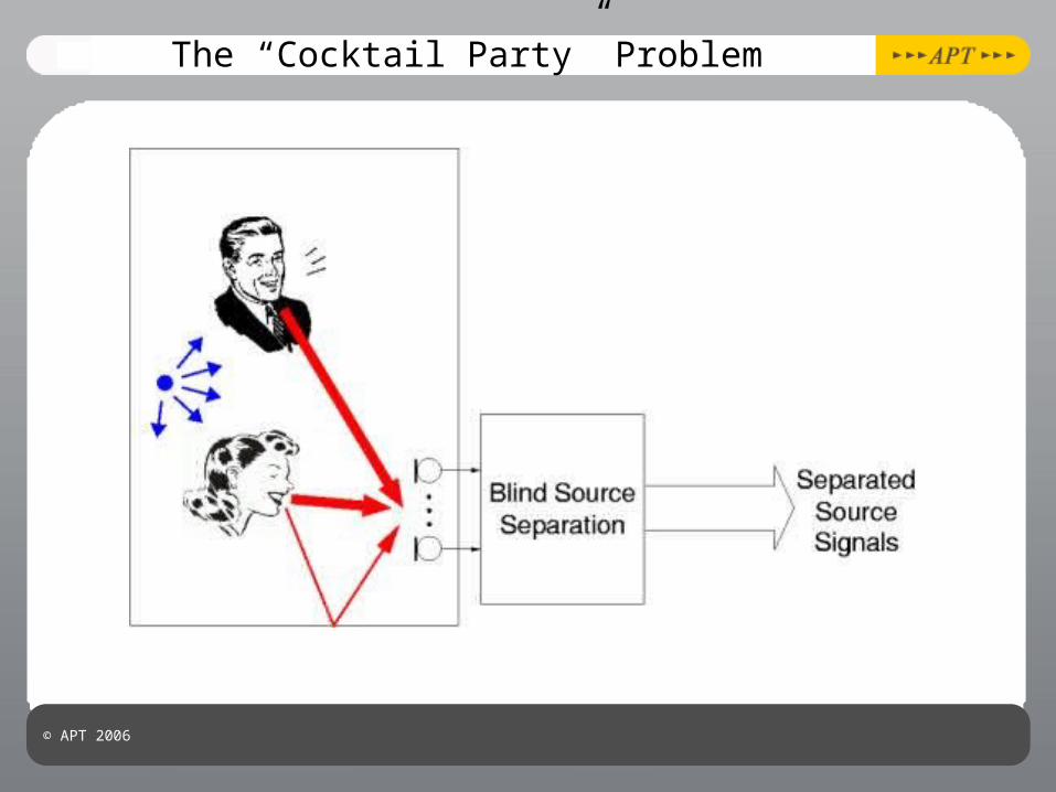
The “Cocktail Party” Problem

© APT 2006

Blind Source Separation

• Can we extract signals based only on the fact that we know they have certain properties?• Fat Tails (kurtosis, higher moments)• Autocorrelation

• Yes! • Principle Components Analysis• Independent Components Analysis• Second Order Blind Identification

• Back and Weigend (1997) were the first to apply ICA to financial data• Useful Adjunct to PCA

• Recent analyses (e.g. Korizis, et. al. (2007)) Have begun to reconsider application of modified, non-independent factorisation algorithms taking into account time series dynamics.

© APT 2006

Independent Component Analysis

• Technique employed for tackling the so-called ‘cocktail party problem’

• Searching for a set of latent variables for whom the joint probability distribution ‘factorises’

• Alternatively, we could formulate this in terms of the moments of the latent variables…

© APT 2006

ICA By Non-Gaussianity

-5 -4 -3 -2 -1 0 1 2 3 4 5-5

-4

-3

-2

-1

0

1

2

3

4

5

Standard Normal Quantiles

Qua

ntile

s of

Inp

ut S

ampl

e

QQ Plot of Sample Data versus Standard Normal

Κ = 11.3 Κ = 13.8

-5 -4 -3 -2 -1 0 1 2 3 4 5-5

-4

-3

-2

-1

0

1

2

3

4

5

Standard Normal Quantiles

Qua

ntile

s of

Inp

ut S

ampl

e

QQ Plot of Sample Data versus Standard Normal

Κ = 6.7

-5 -4 -3 -2 -1 0 1 2 3 4 5-5

-4

-3

-2

-1

0

1

2

3

4

5

Standard Normal Quantiles

Qua

ntile

s of

Inp

ut S

ampl

e

QQ Plot of Sample Data versus Standard Normal

+ =

• Can we employ the central limit theorem to our advantage?

• Consider sums of indepdendent GARCH(1,1) processes

© APT 2006

ICs via Kurtosis?

• First step, pre-processing or “whitening” to generate z.

• Consider linear combinations of z, s, such that some measure of non-Gaussianity, namley f(s) is maximized.

• And optimize by gradient ascent for each signal…

© APT 2006

ICs via Negentropy

• Consider Entropy of a Random Variable

• Well known fact that this is maximal for Gaussian variable.

• As such, maximize “negentropy”

• Statistically-speaking negentropy provides “optimal” discrimination and detection of NonGaussianity

© APT 2006

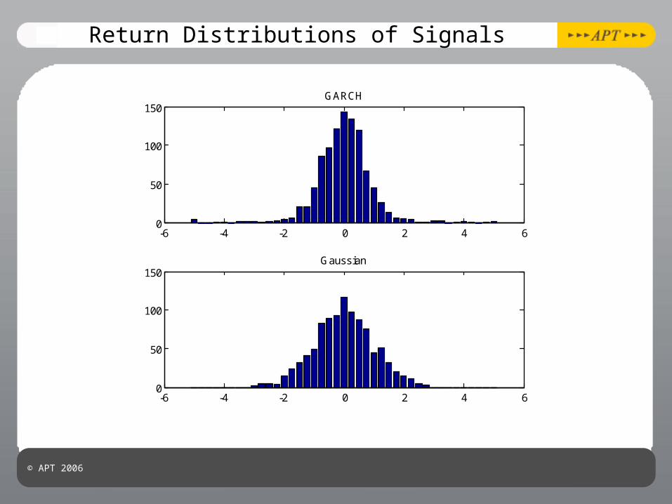
Simple GARCH Test Case

• We generate 1000 returns employing the following two proceses

• With Variances Defined By

• and

• Apply mixing with random matrix M to generate observed signals:

• Can ICA extract the original signals?

© APT 2006

Return Distributions of Signals

-6 -4 -2 0 2 4 60

50

100

150GARCH

-6 -4 -2 0 2 4 60

50

100

150Gaussian

© APT 2006

Distributions of Independent Components

-6 -4 -2 0 2 4 60

50

100

150IC 1

-6 -4 -2 0 2 4 60

50

100

150IC 2

© APT 2006

Scatter Plot

-8 -6 -4 -2 0 2 4 6 8 10-8

-6

-4

-2

0

2

4

6

8GARCH vs IC 1

GARCH

IC 1

Correlation = 0.999

© APT 2006

GARCH Tests

• Extend this analysis in order to accommodate multiple GARCH series

• Try five independent GARCH times series and one Gaussian

• Apply Random Mixing To Generate Observed Signals

0 500 1000-0.05

0

0.05GARCH 1

0 500 1000-0.05

0

0.05GARCH 2

0 500 1000-0.05

0

0.05GARCH 3

0 500 1000-0.02

0

0.02GARCH 4

0 500 1000-0.1

0

0.1GARCH 5

0 500 1000-5

0

5GAUSS

Sources (Latent) Signals (Observed)

0 500 1000-5

0

5MIX 1

0 500 1000-2

0

2MIX 2

0 500 1000-0.5

0

0.5MIX 3

0 500 1000-5

0

5MIX 4

0 500 1000-0.5

0

0.5MIX 5

0 500 1000-5

0

5MIX 6

© APT 2006

GARCH Tests

• Compare Extracted and Original Signals• Amplitudes and Signs Arbitrary

0 500 1000-0.05

0

0.05GARCH 1

0 500 1000-0.05

0

0.05GARCH 2

0 500 1000-0.05

0

0.05GARCH 3

0 500 1000-0.02

0

0.02GARCH 4

0 500 1000-0.1

0

0.1GARCH 5

0 500 1000-5

0

5GAUSS

Sources (Latent)

0 500 1000-10

0

10IC 1

0 500 1000-10

0

10IC 2

0 500 1000-5

0

5IC 3

0 500 1000-10

0

10IC 4

0 500 1000-5

0

5IC 5

0 500 1000-5

0

5IC 6

Components (Extracted)

© APT 2006

GARCH Tests

• Compare Correlations Between Sources and Recovered Components

  IC1 IC2 IC3 IC4 IC5 IC6

G1 -1.00 -0.05 0.01 -0.06 -0.04 0.00

G2 -0.05 -0.14 -0.94 0.27 -0.05 -0.15

G3 0.08 -0.01 -0.31 -0.94 0.11 -0.01

G4 -0.02 -0.09 0.05 0.12 0.99 -0.04

G5 0.06 -0.99 0.07 0.00 -0.06 0.03

G6 -0.02 -0.01 -0.13 0.06 0.10 0.99

© APT 2006

Common Feature Extraction

• Generate Six Time Series

• With the gi defined as before and

© APT 2006

Common Feature Extraction

N=0.1 IC 1 IC 2 IC 3 IC 4 IC 5 IC 6

g1 0.99 0.00 0.06 0.04 -0.04 0.02

g2 0.05 -0.94 -0.31 -0.10 0.01 0.00

g3 -0.09 -0.35 0.92 0.12 -0.07 -0.05

N=0.25 IC 1 IC 2 IC 3 IC 4 IC 5 IC 6

g1 -0.98 -0.01 0.07 -0.04 0.04 -0.02

g2 -0.05 -0.92 -0.32 0.11 0.01 -0.01

g3 0.11 -0.36 0.90 -0.11 0.08 0.09

© APT 2006

Common Feature Extraction

N=0.5 IC 1 IC 2 IC 3 IC 4 IC 5 IC 6

g1 -0.93 0.04 0.09 -0.05 -0.04 0.01

g2 -0.04 0.86 -0.37 0.11 -0.05 0.06

g3 0.13 0.40 0.82 -0.10 -0.09 -0.17

N=1.0 IC 1 IC 2 IC 3 IC 4 IC 5 IC 6

g1 -0.78 0.07 0.05 0.03 -0.05 0.08

g2 -0.02 0.62 -0.45 -0.29 -0.10 -0.05

g3 0.13 0.52 0.53 0.27 -0.13 0.07

© APT 2006

Interpretation of the Mixing Matrix

• Interpret Mixing Matrix, A, for N=0.5

1 2 3 4 5 6-1

0

1Mixture 1 IC Profile

1 2 3 4 5 6-1

0

1Mixture 2 IC Profile

1 2 3 4 5 6-1

0

1Mixture 3 IC Profile

1 2 3 4 5 6-1

0

1Mixture 4 IC Profile

1 2 3 4 5 6-1

0

1Mixture 5 IC Profile

1 2 3 4 5 6-1

0

1Mixture 6 IC Profile

© APT 2006

ICA-Based Clustering

• Very recently, there have been proposals for ICA-based clustering

• Yu & Wu (2006) employ a heuristic-based approach based on thresholded elements of the mixing matrix

• Instead, we employ the L1 norm:

• L1 preserves sensitivity to factor rotation!

• Combine with (standard) clustering algorithms (KMeans, etc…).

© APT 2006

Interpretation of the Mixing Matrix via Clustering

Garch #1

Garch #2

Garch #3

© APT 2006

Reality Check Dataset

• We can confirm the results for a standard “reality check” dataset

• Whether by linkage-based techniques or K-Means, we obtain “correct” clusters

• Not employing time series information (in particular autocorrelation)

• Reduction in dimensionality…

© APT 2006

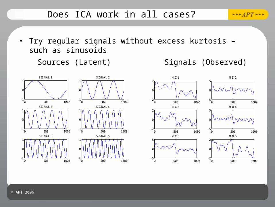
Does ICA work in all cases?

• Try regular signals without excess kurtosis – such as sinusoids

0 500 1000-1

0

1SIGNAL 1

0 500 1000-1

0

1SIGNAL 2

0 500 1000-1

0

1SIGNAL 3

0 500 1000-1

0

1SIGNAL 4

0 500 1000-1

0

1SIGNAL 5

0 500 1000-1

0

1SIGNAL 6

0 500 1000-2

0

2MIX 1

0 500 1000-5

0

5MIX 2

0 500 1000-2

0

2MIX 3

0 500 1000-5

0

5MIX 4

0 500 1000-5

0

5MIX 5

0 500 1000-2

0

2MIX 6

Sources (Latent) Signals (Observed)

© APT 2006

Time Series-Based Methods

• Compare Results for two different methods of signal separation

• ICA-based techniques do not, by default, employ time series information

• Techniques such as SOBI (Second-Order Blind Identification) do, however. (see Korzis, et al. for a related study!)

0 500 1000-5

0

5IC 1

0 500 1000-5

0

5IC 2

0 500 1000-5

0

5IC 3

0 500 1000-5

0

5IC 4

0 500 1000-5

0

5IC 5

0 500 1000-5

0

5IC 6

0 500 1000-2

0

2IC 1

0 500 1000-2

0

2IC 2

0 500 1000-2

0

2IC 3

0 500 1000-2

0

2IC 4

0 500 1000-2

0

2IC 5

0 500 1000-2

0

2IC 6

ICA SOBI (AR(2))

© APT 2006

ICA and HFRX Index Returns

• As a first attempt, can apply ICA to returns of HFRX indices• Looking for dependence on particular components (or

combinations)

Loadings Time Series (Mar 2000 to Feb 2007)

0 20 40 60 80-4

-2

0

2

4IC 1

0 20 40 60 80-4

-2

0

2

4IC 2

0 20 40 60 80-4

-2

0

2

4IC 3

0 20 40 60 80-4

-2

0

2

4IC 4

0 20 40 60 80-4

-2

0

2

4IC 5

0 20 40 60 80-4

-2

0

2

4IC 6

0 20 40 60 80-4

-2

0

2

4IC 7

0 20 40 60 80-4

-2

0

2

4IC 8

1 2 3 4 5 6 7 8-1

0

1HFRX Convertible Arbitrage Index

1 2 3 4 5 6 7 8-1

0

1HFRX Distressed Securities Index

1 2 3 4 5 6 7 8-1

0

1HFRX Equity Hedge Index

1 2 3 4 5 6 7 8-1

0

1HFRX Equity Market Neutral Index

1 2 3 4 5 6 7 8-1

0

1HFRX Event Driven Index

1 2 3 4 5 6 7 8-1

0

1HFRX Macro Index

1 2 3 4 5 6 7 8-1

0

1HFRX Merger Arbitrage Index

1 2 3 4 5 6 7 8-1

0

1HFRX Relative Value Arbitrage Index

© APT 2006

ICA-Based Clustering

Eq Hedge Ev Driv Macro Merger A Conv Arb Dist Secs Rel Val Eq M.N.

1.8

2

2.2

2.4

2.6

2.8

3

© APT 2006

AutoCorrelation in HFRX Index Returns

• Do we see autocorrelation in the returns – is there a time structure in the return or are they temporally independent?

• ICA Doesn’t Consider Temporal Relations

0 1 2 3 4 5-1

0

1

Lag

HFRX Convertible Arbitrage Index

0 1 2 3 4 5-1

0

1

Lag

HFRX Distressed Securities Index

0 1 2 3 4 5-1

0

1

Lag

HFRX Equity Hedge Index

0 1 2 3 4 5-1

0

1

Lag

HFRX Equity Market Neutral Index

0 1 2 3 4 5-1

0

1

Lag

HFRX Event Driven Index

0 1 2 3 4 5-1

0

1

Lag

HFRX Macro Index

0 1 2 3 4 5-1

0

1

Lag

HFRX Merger Arbitrage Index

0 1 2 3 4 5-1

0

1

Lag

HFRX Relative Value Arbitrage Index

0 1 2 3 4 5-1

0

1

Lag

IC 1

0 1 2 3 4 5-1

0

1

Lag

IC 2

0 1 2 3 4 5-1

0

1

Lag

IC 3

0 1 2 3 4 5-1

0

1

Lag

IC 4

0 1 2 3 4 5-1

0

1

Lag

IC 5

0 1 2 3 4 5-1

0

1

Lag

IC 6

0 1 2 3 4 5-1

0

1

Lag

IC 7

0 1 2 3 4 5-1

0

1

Lag

IC 8

HF Autocorrelations IC Autocorrelations

© APT 2006

Second-Order Blind Analysis

• What happens if we explicitly consider autocorrelations?• Results for joint diagonalization of order 2 serial

correlations…

1 2 3 4 5 6 7 8-1

0

1HFRX Convertible Arbitrage Index

1 2 3 4 5 6 7 8-1

0

1HFRX Distressed Securities Index

1 2 3 4 5 6 7 8-1

0

1HFRX Equity Hedge Index

1 2 3 4 5 6 7 8-1

0

1HFRX Equity Market Neutral Index

1 2 3 4 5 6 7 8-1

0

1HFRX Event Driven Index

1 2 3 4 5 6 7 8-1

0

1HFRX Macro Index

1 2 3 4 5 6 7 8-1

0

1HFRX Merger Arbitrage Index

1 2 3 4 5 6 7 8-1

0

1HFRX Relative Value Arbitrage Index

0 20 40 60 80-4

-2

0

2

4SOBI 1

0 20 40 60 80-4

-2

0

2

4SOBI 2

0 20 40 60 80-4

-2

0

2

4SOBI 3

0 20 40 60 80-4

-2

0

2

4SOBI 4

0 20 40 60 80-4

-2

0

2

4SOBI 5

0 20 40 60 80-4

-2

0

2

4SOBI 6

0 20 40 60 80-4

-2

0

2

4SOBI 7

0 20 40 60 80-4

-2

0

2

4SOBI 8

Loadings Time Series (Mar 2000 to Feb 2007)

© APT 2006

SOBI-Based Clustering

Eq Hedge Ev Driv Merger A Rel Val Conv Arb Dist Secs Macro Eq M.N.

1.8

2

2.2

2.4

2.6

2.8

3

© APT 2006

AutoCorrelation in HFRX Index Returns

• SOBI performs a joint decomposition based on the autocorrelation structure of the candidate signals

0 1 2 3 4 5-1

0

1

Lag

HFRX Convertible Arbitrage Index

0 1 2 3 4 5-1

0

1

Lag

HFRX Distressed Securities Index

0 1 2 3 4 5-1

0

1

Lag

HFRX Equity Hedge Index

0 1 2 3 4 5-1

0

1

Lag

HFRX Equity Market Neutral Index

0 1 2 3 4 5-1

0

1

Lag

HFRX Event Driven Index

0 1 2 3 4 5-1

0

1

Lag

HFRX Macro Index

0 1 2 3 4 5-1

0

1

Lag

HFRX Merger Arbitrage Index

0 1 2 3 4 5-1

0

1

Lag

HFRX Relative Value Arbitrage Index

HF Autocorrelations SOBI Autocorrelations

0 1 2 3 4 5-1

0

1

Lag

SOBI 1

0 1 2 3 4 5-1

0

1

Lag

SOBI 2

0 1 2 3 4 5-1

0

1

Lag

SOBI 3

0 1 2 3 4 5-1

0

1

Lag

SOBI 4

0 1 2 3 4 5-1

0

1

Lag

SOBI 5

0 1 2 3 4 5-1

0

1

Lag

SOBI 6

0 1 2 3 4 5-1

0

1

Lag

SOBI 7

0 1 2 3 4 5-1

0

1

Lag

SOBI 8

© APT 2006

Conclusions

• Correct Specification of factor models is vital

• Interpretation of Statistical Factors and Higher-Order Effects

• Latent Variable Estimation and Study• Blind Source Separation• Non-Gaussianity• Time-Series Models

• Future Directions• Out of Sample Tests of Higher Moments• Simulation / Risk Modelling

© APT 2006

References

• Hyvarinen, et al., Independent Component Analysis, Wiley, Ney York (2001).

• A.D. Back and A.S. Weigend, “A first application of independent component analysis to extracting structure from stock returns”, Int. Journal of Neural Systems, Vol. 8, No. 4, Aug. 1997 , pp. 473-484.

• A. Beloucharnai, et al., “A blind source separation technique based on second order statistics”. IEEE Trans. On Signal Processing, Vol. 45, No. 2, pp. 434-444, (1997).

• H. C. Wu a; Philip L. H. Yu, “A robust and scalable clustering model for time series via independent component analysis.”, International Journal of Systems Science, Volume 37, No. 13, October 2006 , pages 987 - 1001

• Korizis, et. al., Smooth Component Extraction From a Set of Finanacial Financial Data Mixtures, Proceedings of the Fourth IASTED International Conference on Signal Processing, Pattern Recognition, and Applications (2007).

• E. Keogh and T. Folias, ‘‘The UCR Time Series Data Mining Archive’’, [http://www.cs.ucr.edu/eamonn/TSDMA/index.html]. Riverside CA. University of California – Computer Science & Engineering Department, 2002