§ / Applied Bayesian Inference, KSU, April 29, 2012 §❺ Metropolis-Hastings sampling and general...

§ /

Applied Bayesian Inference, KSU, April 29, 2012

1

§❺ Metropolis-Hastings sampling and general MCMC approaches for GLMM

Robert J. Tempelman

§ /


2

Genetic linkage example…again

Recall plant genetic linkage analysis problem

or

Suppose flat constant prior (p(q) 1) was used. Then

4321

44

1

4

1

4

2

!!!!

!|

4321

yyyy

yyyy

nL

y

4321 112| yyyyL y

R

dL

Lp

y

yy

|

||

§ /


3

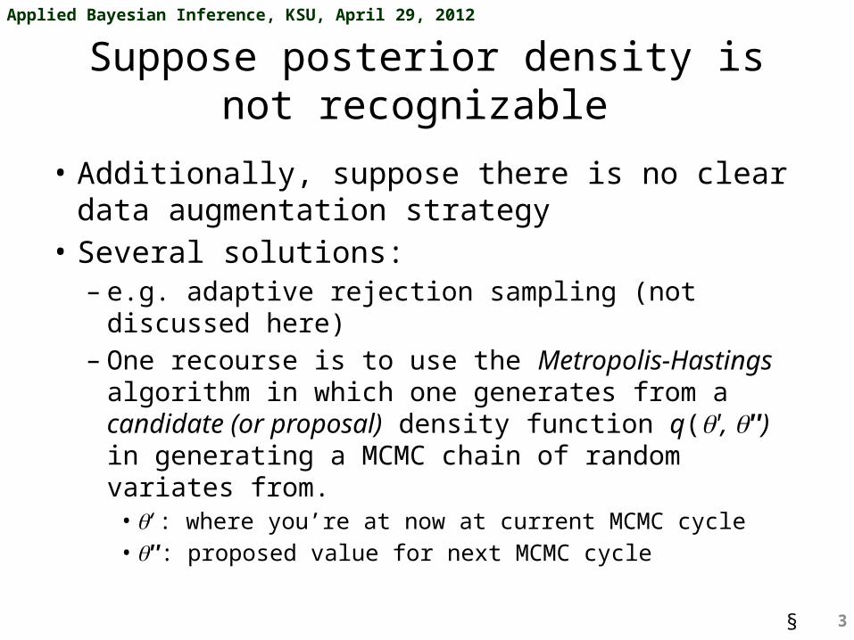
Suppose posterior density is not recognizable

• Additionally, suppose there is no clear data augmentation strategy

• Several solutions:– e.g. adaptive rejection sampling (not discussed here)– One recourse is to use the Metropolis-Hastings

algorithm in which one generates from a candidate (or proposal) density function q(q', q'') in generating a MCMC chain of random variates from.

• q‘ : where you’re at now at current MCMC cycle• q'': proposed value for next MCMC cycle

§ /


4

Metropolis Hastings

• Say MCMC cycle is currently at value q[t-1] from cycle t-1.

• Draw a proposed value q* from candidate density for cycle t.

• Accept move from q[t-1] to q[t] = q* with probability:

– Otherwise set q[t] = q*

0*,|*

,1

1,*,|

*,|*min

*, ]1[]1[]1[

]1[

]1[

ttt

t

t qpif

otherwiseqp

qp

y y

y

[ 1] , *tq

Good readable reference? Chib and Greenburg (1995)

§ /


5

How to compute this ratio “safely”

• Always use logarithms whenever evaluating ratios!!!

• Once you compute this…then backtransform

[ 1]

[ 1] [ 1]

[ 1] [ 1] [ 1]

* | *,log log

| , *

log * | log *, log | log , *

y

y

y y

t

t t

t t t

p q

p q

p q p q

exp log

§ /


6

Back to plant genetics exampleRecall y1=1997, y2=906, y3=904, y4=32.

Let’s use as the candidate generating function (based on likelihood approx.)1.Determine a starting value (i.e. 0th cycle) q[o]

2.For t = 1, m (number of MCMC cycles)a) Generate q * from q(q[t-1], q*) = N(0.0357,3.6338 x 10-5) b) Generate U from a Uniform(0,1) distributionc) If U<a(q[t-1], q*) then set q[t]= q *, else set q[t] = q[t-1]

• Note that this is an independence chains algorithm

q(q[t-1], q*) = N( =m 0.0357, s2 = 3.6338 x 10-5)

q(q[t-1], q*) = q(q*)

§ /


7

Independence chains Metropolis

• When candidate does not depend on q[t-1]

– i.e.

• However, in spite of this “independence” label, there is still serial autocorrelation between the samples.

• IML code online. Generate output for 9000 draws after 1000 burn-in samples. Save every 10.

0*|

,1

1,*|

|*min

*, ]1[]1[

]1[

]1[

qpif

otherwiseqp

qp

tt

t

t y y

y

q(q[t-1], q*) = q(q*)

§ /


8

Key plots and summaries

§ /


9

Monitoring MH acceptance rates over cycles for genetic linkage example

• Average MH acceptance rates (for every 10 cycles)

ALPHASAV

0.0

0.1

0.2

0.3

0.4

0.5

0.6

0.7

0.8

0.9

1.0

CYCLE

1000 2000 3000 4000 5000 6000 7000 8000 9000 10000

Many acceptance rates close to 1!

Is this good?

NO

Intermediate acceptance ratios (0.25-0.5) are optimal for MH mixing.

§ /


10

How to optimize Metropolis acceptance ratios

• Recall q(q[t-1], q*) = N(m,s2)– m = 0.0357, s2=3.6338 x 10-5

• Suggest using q(q[t-1], q*) = N(m,cs2) and modify c (during burn-in) so that MH acceptance rates are intermediate– Increase c ….decrease acceptance rates– Decrease c ….increase acceptance rates.

§ /


11

“Tuning” the MH-sampler:My strategy

• Every 10 MH cycles for first half of burnin, assess the following:– if average acceptance rate > .80, then set c = 1.2 c,– if average acceptance rate < .20 then set c = 0.7 c,– otherwise let c be.

• SAS PROC MCMC has a somewhat different strategy.

• Let’s rerun same PROC IML code again but with this modification.

§ /


12

Average acceptance ratio versus cycle(during 400 burn-in cycles)

C_CHG

1

2

3

4

5

6

7

CYCLE_SCALE

0 1000 2000 3000 4000

c

cycle

One should finish the tuning process not much later than half-ways through “burnin”

§ /


13

Monitoring MH acceptance rates over cycles

• Average MH acceptance rates (every 10 cycles) post burn-in (16000 cycles)

ALPHASAV

0.0

0.1

0.2

0.3

0.4

0.5

0.6

0.7

0.8

0.9

1.0

CYCLE

4000 5000 6000 7000 8000 9000 10000 11000 12000 13000 14000 15000 16000 17000 18000 19000 20000

§ /


14

Posterior density of q.

Analysis Variable : theta

Mean Median Std Dev 5th Pctl 95th Pctl

0.0366 0.0366 0.0064 0.0265 0.0471

§ /


15

Random walk Metropolis sampling• More common (especially when proposals based

on likelihood function are not plausible) than independence chains Metropolis.

• Proposal density is chosen to be symmetric in q* and q[t-1].– i.e. q(q[t-1], q*) = q(q*, q[t-1])

• Example: generate a random variate d from N(0,cs2) and add it to the previous cycle value q[t-1] to generate q* = q[t-1] + d: same as sampling from

]1[']1[

22

]1[ **2

1exp

2

1*, ttt

ccq

§ /


16

Random walk Metropolis (cont’d)

• Because of symmetricity of q(q[t-1], q*) in q[t-

1] and q*, MH acceptance ratio simplifies:

• i.e., because

0|

,1

1,|

|*min

*, ]1[]1[]1[

y y

yttt pif

otherwisep

p

[ 1] [ 1], * *,t tq q

§ /


17

Back to example.

• Start again with s2 = 0.00602 and a starting value for q[t-1] at t=1.

• Generate proposed value from

accept with probability

– i.e., generate from N(0,cs2) and add to q[t-1] • Tune c for intermediate acceptance rates during burn-in.

]1[']1[

22

]1[ **2

1exp

2

1*, ttt

ccq

0|

,1

1,|

|*min

*, ]1[]1[]1[

y y

yttt pif

otherwisep

p

§ /


18

Summary

§ /


19

What about “canned” software?

• WinBugs• AD Model Builder• Various R packages (MCMCglmm)• SAS PROC MCMC

– Will demonstrate shortly…functions a bit like PROC NLINMIXED (no class statement)

• They all work fine.– But sometimes they don’t recognize conjugacy in priors

• i.e., can’t distinguish between conjugate and non-conjugate (Metropolis) sampling.

• So often defaults to Metropolis. (PROC MCMC: random walk Metropolis)

§ /


20

Recall old split plot in time example

• Recall the “bunny” example from earlier.– We used PROC GLIMMIX and MCMC (SAS PROC IML) to

analyze the data.– Our MCMC implementation involved recognizeable FCD

• Split plot in time assumption.– Other alternatives?

• Marginal versus conditional specifications on CS• AR(1)• Others?

– Some FCD are not recognizeable• Metropolis updates necessary.• Let’s use SAS PROC MCMC.

§ /


21

First create the dummy variables using PROC TRANSREG (PROC MCMC does not have a “CLASS” statement)

(Dataset called ‘recodedsplit’)Obs _NA

ME_Intercept

trt1 trt2 time1

time2

time3

Trt1time1

Trt1time2

Trt1time3

Trt2time1

Trt2time2

Trt2time3

trt time y trtrabbit

1 -0.3 1 1 0 1 0 0 1 0 0 0 0 0 1 1 -0.3 1_1

2 -0.2 1 1 0 0 1 0 0 1 0 0 0 0 1 2 -0.2 1_1

3 1.2 1 1 0 0 0 1 0 0 1 0 0 0 1 3 1.2 1_1

4 3.1 1 1 0 0 0 0 0 0 0 0 0 0 1 4 3.1 1_1

5 -0.5 1 1 0 1 0 0 1 0 0 0 0 0 1 1 -0.5 1_2

6 2.2 1 1 0 0 1 0 0 1 0 0 0 0 1 2 2.2 1_2

7 3.3 1 1 0 0 0 1 0 0 1 0 0 0 1 3 3.3 1_2

8 3.7 1 1 0 0 0 0 0 0 0 0 0 0 1 4 3.7 1_2

9 -1.1 1 1 0 1 0 0 1 0 0 0 0 0 1 1 -1.1 1_3

10 2.4 1 1 0 0 1 0 0 1 0 0 0 0 1 2 2.4 1_3

Part of X matrix (full-rank) &_trgind

§ /


22

SAS PROC MCMC(“Conditional” specification)

proc mcmc data=recodedsplit outpost=ksu.postsplit propcov=quanew seed = &seed nmc=400000 thin=10monitor = (beta1-beta&nvar sigmae sigmag); array covar[&nvar] intercept &_trgind; array beta[&nvar] ; parms sige 1 ; * residual sd; parms sigg 1 ; * random ef sd; parms (beta1-beta&nvar) 1;

prior beta:~normal(0,var=1e6);/* prior beta: ~ general(0); could also do this too */ prior sige ~ general(0,lower=0); /* Gelman prior */ prior sigg ~ general(0,lower=0); /* Gelman prior */

Where to save the MCMC samples

Metropolis implementation strategy

data null; call symputx(‘seed', 8723); call symputx('nvar',12); run;

Save how often?

Total number of samples after burnin

NBI = 1000 (default number of burn-in cycles)

Fixed effects dummy variables

Fixed effects

Parms: starting values

Priors: b ~ N(0,106)p(se) ~ constant;p(su) ~ constant

§ /


23

SAS PROC MCMC(conditional specification)

beginnodata; sigmae = sige*sige; sigmau = sigg*sigg; endnodata;

call mult(covar, beta, mu); random u ~ normal (0,var=sigmau) subject=trtrabbit ; model y ~ normal(mu + u,var=sigmae);run;

'x βi i

' ' 2,x β z ui i i ey N 20,i uu N

22u u

22e e

§ /


24

PROC MCMC outputParametersBlock Parameter Sampling

MethodInitialValue

Prior Distribution

1 sige N-Metropolis 1.0000 general(0,lower=0)

2 sigg N-Metropolis 1.0000 general(0,lower=0)

3 beta1 N-Metropolis 1.0000 normal(0,var=1e6)

beta2 1.0000 normal(0,var=1e6)











Random Effects Parameters

Parameter Subject Levels Prior Distribution

u trtrabbit 15 normal(0,var=sigmau)

§ /


25

Posterior Summaries

Parameter N Mean StandardDeviation

Percentiles

25% 50% 75%

beta1 40000 0.2178 0.3910 -0.0434 0.2199 0.4823

beta2 40000 2.3706 0.5528 2.0007 2.3707 2.7360

beta3 40000 -0.2079 0.5524 -0.5761 -0.2063 0.1545

beta4 40000 -0.8958 0.5086 -1.2292 -0.8967 -0.5616

beta5 40000 0.0139 0.5066 -0.3172 0.0115 0.3501

beta6 40000 -0.6407 0.5006 -0.9753 -0.6429 -0.3033

beta7 40000 -1.9340 0.7151 -2.4049 -1.9339 -1.4548

beta8 40000 -1.2282 0.7134 -1.7030 -1.2309 -0.7548

beta9 40000 -0.0719 0.7071 -0.5445 -0.0763 0.3993

beta10 40000 0.3055 0.7127 -0.1721 0.3011 0.7832

beta11 40000 -0.5411 0.7097 -1.0132 -0.5395 -0.0682

beta12 40000 0.5758 0.7033 0.1095 0.5748 1.0406

sigmae 40000 0.6314 0.1478 0.5266 0.6124 0.7148

sigmau 40000 0.1276 0.1465 0.0285 0.0850 0.1748

Compare to conditional model results from § 82,84

§ /


26

Effective Sample Sizes

Parameter ESS AutocorrelationTime

Efficiency

beta1 4285.7 9.3334 0.1071

beta2 5778.0 6.9229 0.1444

beta3 5171.1 7.7353 0.1293

beta4 5639.7 7.0926 0.1410

beta5 3900.5 10.2550 0.0975

beta6 3901.6 10.2522 0.0975

beta7 4197.4 9.5297 0.1049

beta8 6248.7 6.4013 0.1562

beta9 6857.7 5.8329 0.1714

beta10 2890.5 13.8385 0.0723

beta11 6647.5 6.0173 0.1662

beta12 5563.2 7.1902 0.1391

sigmae 6173.6 6.4792 0.1543

sigmau 1364.3 29.3186 0.0341

§ /


27

LSMEANS USING PROC MIXED

trt Least Squares Means

trt Estimate Standard Error

1 1.4000 0.2135

2 -0.2900 0.2135

3 -0.1600 0.2135

time Least Squares Means

time Estimate Standard Error

1 -0.5000 0.2100

2 0.3667 0.2100

3 0.4667 0.2100

4 0.9333 0.2100

trt*time Least Squares Means

trt time Estimate Standard Error

1 1 -0.2400 0.3638

1 2 1.3800 0.3638

1 3 1.8800 0.3638

1 4 2.5800 0.3638

2 1 -0.5800 0.3638

2 2 -0.5200 0.3638

2 3 -0.06000 0.3638

2 4 5.5E-15 0.3638

3 1 -0.6800 0.3638

3 2 0.2400 0.3638

3 3 -0.4200 0.3638

3 4 0.2200 0.3638

§ /


28

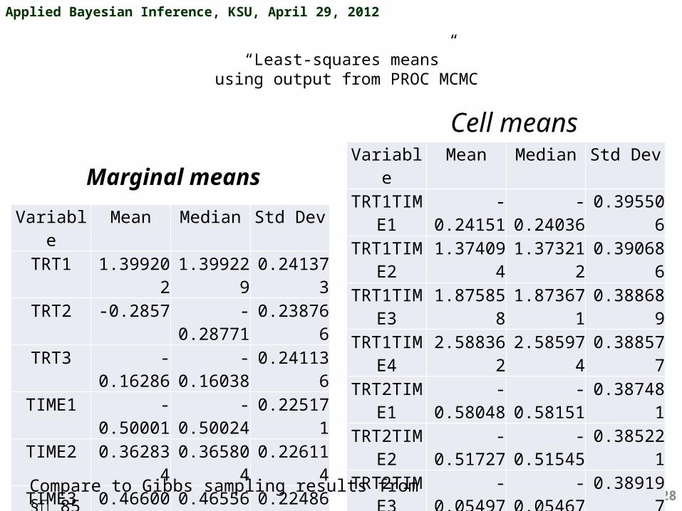
“Least-squares means”using output from PROC MCMC

Variable Mean Median Std DevTRT1 1.399202 1.399229 0.241373TRT2 -0.2857 -0.28771 0.238766TRT3 -0.16286 -0.16038 0.241136

TIME1 -0.50001 -0.50024 0.225171TIME2 0.362834 0.365804 0.226114TIME3 0.466009 0.465563 0.224869TIME4 0.938682 0.937432 0.223448

Variable Mean Median Std DevTRT1TIME1 -0.24151 -0.24036 0.395506TRT1TIME2 1.374094 1.373212 0.390686TRT1TIME3 1.875858 1.873671 0.388689TRT1TIME4 2.588362 2.585974 0.388577TRT2TIME1 -0.58048 -0.58151 0.387481TRT2TIME2 -0.51727 -0.51545 0.385221TRT2TIME3 -0.05497 -0.05467 0.389197TRT2TIME4 0.0099 0.008927 0.389475TRT3TIME1 -0.67805 -0.67985 0.393538TRT3TIME2 0.231677 0.2315 0.395277TRT3TIME3 -0.42287 -0.41975 0.38795TRT3TIME4 0.217785 0.219946 0.390986

Marginal means

Cell means

Compare to Gibbs sampling results from § 85

§ /


29

Posterior densities of s2u s2

e

Bounded above 0…by definition

§ /


30

The Marginal Model Specification (Type = CS)

• SAS PROC MIXED CODE

title "Marginal Model: Compound Symmetry using PROC MIXED";proc mixed data=ear ; class trt time rabbit; model temp = trt time trt*time /solution; repeated time /subject = rabbit(trt) type=cs rcorr; lsmeans trt*time;run;

§ /


31

• Now

• To ensure R is p.s.d,– nt: number of repeated measures per rabbit

2 2 2 2 2

2 2 2 2 22

( ) 2 2 2 2 2

2 2 2 2 2

1

1

1

1

R

u e u u u

u u e u uk i

u u u e u

u u u u e

2

2 2u

u e

2 2 2

u e

1

11

tn

§ /


32

Need to format data differentlyObs trt time trtrabbit first last y

1 1 1 1_1 1 0 -0.3

2 1 2 1_1 0 0 -0.2

3 1 3 1_1 0 0 1.2

4 1 4 1_1 0 1 3.1

5 1 1 1_2 1 0 -0.5

6 1 2 1_2 0 0 2.2

7 1 3 1_2 0 0 3.3

8 1 4 1_2 0 1 3.7

9 1 1 1_3 1 0 -1.1

10 1 2 1_3 0 0 2.4

data=recodedsplit1

§ /


33

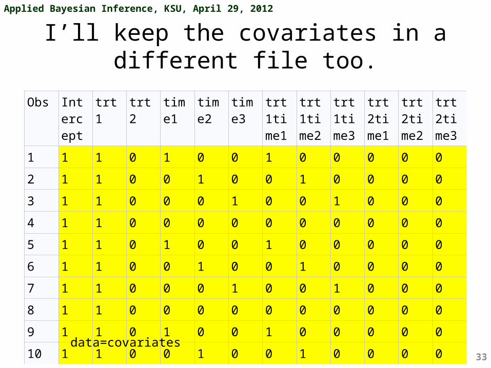
I’ll keep the covariates in a different file too.

Obs Intercept

trt1 trt2 time1

time2

time3

trt1time1

trt1time2

trt1time3

trt2time1

trt2time2

trt2time3

1 1 1 0 1 0 0 1 0 0 0 0 0

2 1 1 0 0 1 0 0 1 0 0 0 0

3 1 1 0 0 0 1 0 0 1 0 0 0

4 1 1 0 0 0 0 0 0 0 0 0 0

5 1 1 0 1 0 0 1 0 0 0 0 0

6 1 1 0 0 1 0 0 1 0 0 0 0

7 1 1 0 0 0 1 0 0 1 0 0 0

8 1 1 0 0 0 0 0 0 0 0 0 0

9 1 1 0 1 0 0 1 0 0 0 0 0

10 1 1 0 0 1 0 0 1 0 0 0 0

data=covariates

§ /


34

PROC MCMCdata a; run;

/* PROC MCMC WITH COMPOUND SYMMETRY ASSUMPTION */title1 "Bayesian inference on compound symmetry ";proc mcmc jointmodel data=a outpost=ksu.postcs propcov=quanew seed = &seed nmc=400000 thin=10 ;

array covar[1]/nosymbols ; array data[1]/nosymbols; array first1[1]/nosymbols; array last1[1]/nosymbols;

array beta[&nvar] ; array mu[&nrec]; array ytemp[&nrep]; array mutemp[&nrep]; array VCV[&nrep,&nrep];

This data step is a little silly but it is required.

jointmodel option implies that each observation contribution to likelihood function is NOT conditionally independent.

§ /


35

begincnst; rc = read_array("recodedsplit1",data,"y"); rc = read_array("recodedsplit1",first1,"first"); rc = read_array("recodedsplit1",last1,"last"); rc = read_array("covariates",covar);endcnst;

parms sige .25 ; * residual sd; parms intrcl .3 ; * intraclass correlation;

parms (beta1-beta&nvar) 1;

§ /


36

beginnodata; prior beta:~normal(0,var=1e6); prior sige ~ general(0, lower=0); /* Gelman prior */ prior intrcl ~ general(0,lower=&lbound1,upper=.999); sigmae = sige*sige; sigmag = intrcl*sigmae; call fillmatrix(VCV,sigmag);

do i = 1 to &nrep; VCV[i,i] = sigmae;end;call mult(covar,beta,mu);

endnodata;

ljointpdf = 0;

• &lbound1 = -1/3 (lower bound on CS correlation when blocksize = 4)

§ /


37

do irec = 1 to &nrec; if (first1[irec] = 1) then counter=0;

counter = counter + 1; ytemp[counter] = data[irec]; mutemp[counter] = mu[irec]; if (last1[irec] = 1) then do; do; ljointpdf = ljointpdf + lpdfmvn(ytemp, mutemp, VCV); end; end;

end; model general(ljointpdf);run;

§ /


38

PROC MCMCPosterior Summaries

Parameter N Mean StandardDeviation

Percentiles

25% 50% 75%

sige 40000 0.8643 0.1040 0.7921 0.8528 0.9225

intrcl 40000 0.1736 0.1453 0.0679 0.1599 0.2661

beta1 40000 0.2267 0.3909 -0.0313 0.2298 0.4869

beta2 40000 2.3553 0.5523 1.9916 2.3491 2.7140

beta3 40000 -0.2290 0.5536 -0.5965 -0.2327 0.1388

beta4 40000 -0.8982 0.5012 -1.2320 -0.8984 -0.5682

beta5 40000 0.0185 0.4937 -0.3080 0.0204 0.3433

beta6 40000 -0.6505 0.4985 -0.9830 -0.6529 -0.3221

beta7 40000 -1.9185 0.7058 -2.3900 -1.9170 -1.4498

beta8 40000 -1.2292 0.7038 -1.6901 -1.2329 -0.7667

beta9 40000 -0.0599 0.7024 -0.5232 -0.0555 0.4045

beta10 40000 0.3204 0.7087 -0.1426 0.3182 0.7891

beta11 40000 -0.5386 0.7072 -0.9975 -0.5438 -0.0748

beta12 40000 0.5890 0.7025 0.1227 0.5945 1.0596

§ /


39

PROC MIXED vs PROC MCMC

Covariance Parameter Estimates

Cov Parm Subject Estimate Standard Error

Z Value Pr Z

CS rabbit(trt) 0.08336 0.09910 0.84 0.4002

Residual 0.5783 0.1363 4.24 <.0001

Variable Median Std Dev Minimum Maximum

sigmau2 0.110874 0.15354 -0.34127 5.535211

sigmae2 0.592512 0.152743 0.246462 1.870365

PROC MCMC

PROC MIXED

§ /


40

Posterior marginal densities for s2u and s2

e under marginal model

Notice how much of the posterior density of s2

u is concentrated to the left of 0!

Potential “ripple effect” on inferences on K’b ? (Stroup and Littell., 2002) relative to conditional spec.?

§ /


41

First order autoregressive model (type = AR(1))

• SAS PROC MIXED CODE

title "Marginal Model: AR(1) using PROC MIXED";proc mixed data=ear ; class trt time rabbit; model temp = trt time trt*time /solution; repeated time /subject = rabbit(trt) type= AR(1) rcorr; lsmeans trt*time;run; CORRECTION!

§ /


42

Specifying VCV for AR(1)

• Note

• Might be easier to specify:

2 3

22

( ) 2

3 2

1

1

1

1

Rk i

2

1( ) 2 2 2

1 0 0

1 0 1

0 1 1

0 0 1

Rk i

Especially for large Rk(i)

Example MCMC code provided online.

§ /


43

Variance Component InferenceCovariance Parameter Estimates

Cov Parm Subject Estimate Standard Error

AR(1) rabbit(trt) 0.2867 0.1453

Residual 0.6551 0.141

Variable Median Std Dev 5th Pctl 95th Pctl

rho 0.286 0.149 0.0313 0.52

sigmae2 0.706 0.178 0.501 1.056

PROC MIXED MCMC

§ /


44

An example of a “sticky” situation

• Consider a Poisson (count data) example.• Simulated data from a split plot design.

– 4 whole plots per each of 3 levels of a whole plot factor.

• 3 subplots per whole plot -> 3 levels of a subplot factor.

• Whole plot variance: s2w = 0.50

• Overdispersion (G-side) variance:– B*wholeplot variance: s2

e = 1.00

§ /


45

GLIMMIX code:

proc glimmix data=splitplot method=laplace; class A B wholeplot subject ; model y = A|B /dist=poisson solution ; random wholeplot(A) B*wholeplot(A); lsmeans A B A*B/e ilink;run;

§ /


46

Inferences on variance components:

• PROC GLIMMIX

Covariance Parameter Estimates

Cov Parm Estimate Standard Error

wholeplot(A) 0.6138 0.3516

B*wholeplot(A) 0.9293 0.2514

§ /


47

Using PROC MCMCproc mcmc data=recodedsplit outpost=postout propcov=quanew seed = 9548 nmc=400000 thin=10; array covar[&nvar] intercept &_trgind; array beta[&nvar] ; parms sigmau .5; parms sigmae .5; parms (beta1-beta&nvar) 1; prior beta: ~ normal(0,var=10E6); prior sigmae ~ igamma(shape=.1,scale=.1); prior sigmau ~ igamma(shape=.1,scale=.1); call mult(covar, beta, mu); random u~ normal (0,var=sigmau) subject=plot ; random e~ normal (0,var=sigmae) subject= subject; lambda = exp(mu + u + e); model y ~ poisson(lambda);run;

'x βi i 20,j uu N

' 'exp x β z ui i i ie 20,i ee N

~i iy Poisson

2 0.1,0.1u IG 2 0.1,0.1e IG 6~ ,10β 0 IN

§ /


48

Some outputPosterior Summaries

Parameter

N Mean StandardDeviation

Percentiles

25% 50% 75%

sigmag 40000 0.7947 0.5956 0.3891 0.6635 1.0324

sigmae 40000 1.4055 0.4559 1.0802 1.3285 1.6449

beta1 40000 6.6630 0.3811 6.4611 6.6790 6.9158

beta2 40000 -3.8229 0.8258 -4.3769 -3.8290 -3.2845

beta3 40000 -4.2165 0.8073 -4.7672 -4.2412 -3.7257

beta4 40000 -0.7618 0.4472 -1.0997 -0.8095 -0.4266

beta5 40000 -1.5901 0.6757 -2.1210 -1.5089 -1.1206

beta6 40000 -2.0756 0.7286 -2.5323 -2.0938 -1.6069

beta7 40000 0.7144 1.1396 -0.0554 0.7189 1.4600

beta8 40000 0.6214 1.1488 -0.1162 0.6336 1.3851

beta9 40000 2.4683 1.0499 1.8227 2.4922 3.1429

beta10 40000 1.9011 1.1083 1.2645 1.9517 2.6003

beta11 40000 -0.8063 0.8887 -1.4099 -0.8112 -0.2278

beta12 40000 1.3887 0.9450 0.6332 1.4562 2.0298

In the same ball-park as the PROC GLIMMIX solutions/VC estimates…but there is a PROBLEM ->>>>>

§ /


49

Pretty slow mixingEffective Sample Sizes


Efficiency

sigmag 155.1 257.9 0.0039

sigmae 186.2 214.8 0.0047

beta1 43.0 931.1 0.0011

beta2 59.4 673.8 0.0015

beta3 61.8 646.8 0.0015

beta4 44.1 906.0 0.0011

beta5 42.5 940.4 0.0011

beta6 54.4 735.8 0.0014

beta7 62.5 639.9 0.0016

beta8 86.9 460.1 0.0022

beta9 58.6 682.1 0.0015

beta10 136.2 293.7 0.0034

beta11 53.7 745.5 0.0013

beta12 49.3 811.0 0.0012

§ /


50

sigmag

sigmae

beta1

beta2

§ /


51

From SAS log file:

Too sticky!!! Solution? Thin even more than saving every 10….and generate a lot more samples!

§ /


52

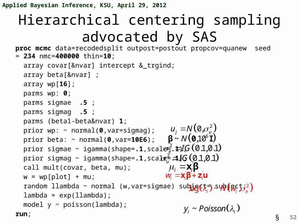
Hierarchical centering sampling advocated by SAS

proc mcmc data=recodedsplit outpost=postout propcov=quanew seed = 234 nmc=400000 thin=10; array covar[&nvar] intercept &_trgind; array beta[&nvar] ; array wp[16]; parms wp: 0; parms sigmae .5 ; parms sigmag .5 ; parms (beta1-beta&nvar) 1; prior wp: ~ normal(0,var=sigmag); prior beta: ~ normal(0,var=10E6); prior sigmae ~ igamma(shape=.1,scale=.1); prior sigmag ~ igamma(shape=.1,scale=.1); call mult(covar, beta, mu); w = wp[plot] + mu; random llambda ~ normal (w,var=sigmae) subject= subject; lambda = exp(llambda); model y ~ poisson(lambda);run;

20,j uu N 6~ ,10β 0 IN 2 0.1,0.1e IG 2 0.1,0.1u IG 'x βi i

' 'x β z ui i iw

~i iy Poisson

2log ~ ,i i eN w

§ /


53

Faster mixing!Effective Sample Sizes


Efficiency

wp1 497.2 80.4554 0.0124wp2 621.5 64.3569 0.0155wp3 336.4 118.9 0.0084wp4 669.9 59.7148 0.0167wp5 967.1 41.3624 0.0242wp6 1767.9 22.6263 0.0442wp7 1160.7 34.4624 0.0290wp8 1109.0 36.0701 0.0277wp9 1275.3 31.3651 0.0319wp10 717.9 55.7176 0.0179wp11 1518.0 26.3512 0.0379wp12 1223.3 32.6995 0.0306wp13 583.9 68.5094 0.0146wp14 606.2 65.9881 0.0152wp15 674.1 59.3384 0.0169wp16 799.2 50.0492 0.0200

Effective Sample Sizes


Efficiency

sigmae 3831.5 10.4397 0.0958sigmag 825.1 48.4794 0.0206beta1 850.1 47.0507 0.0213beta2 1475.5 27.1103 0.0369beta3 908.7 44.0188 0.0227beta4 907.1 44.0954 0.0227beta5 6352.5 6.2967 0.1588beta6 4736.8 8.4446 0.1184beta7 8021.8 4.9864 0.2005beta8 4565.9 8.7606 0.1141beta9 7303.8 5.4766 0.1826beta10 8076.8 4.9525 0.2019beta11 5080.2 7.8738 0.1270beta12 4005.2 9.9870 0.1001

§ /


54

sigmag

sigmae

beta1

beta2

§ /


55

Natural next step

• Compute marginal/cell means as function of effects (b)…just like before.– i.e., k’b

• Transform to the observed scale and look at posterior distribution:– Naturally(?): exp(k’b)

• But that is a “conditional specification”

– Marginally; it might be something different…..

§ /


56

Simple illustration of marginal versus conditional in overdispersed Poisson

• If Yi ~ Poisson (exp(m+ui)) then marginally

so we probably should look at this posterior density of this function instead for “population-averaged” inference.

• Conditionally on ui = 0

• Implications on what functions we look at for posterior distributions.

2

E exp exp2E

i

ui i

u

Y u

E | 0 expi iY u “subject-specific” inference

§ /


57

Enough with your probit link!

• I WANT TO DO MCMC ON A LOGISTIC MIXED EFFECTS MODEL.– I’m an odd(s ratio) kind of guy/girl. – Ok..fine. See worked out example for PROC

MCMC.• Chen Fang. 2011. The RANDOM statement and more:

moving on with PROC MCMC. SAS Global Forum 2011. http://support.sas.com/rnd/app/papers/abstracts/334-2011.html

http://support.sas.com/rnd/app/papers/abstracts/334-2011.html



§ /


58

Other SAS procedures doing Bayesian/MCMC inference?

• Yes, but primarily for fixed effects models.– PROC GENMOD, LIFEREG, PHREG.– Greater need might be for mixed model versions.

• PROC MIXED has some Bayesian MCMC capabilities for simple variance component models.– i.e., not repeated measures.

§ /


59

Repeated measures in generalized linear mixed models

• The G-Side versus R-side conundrum• In classical GLMM analyses (PROC GLMM,

GENMOD), the R-side process cannot be simulated.– Model is “vacuous” (Walt Stroup).

• So take the G-side route.– This would be easy to analyze using MCMC if

underlying liabilities were augmented (need a multivariate normal cdf otherwise).

§ / Applied Bayesian Inference, KSU, April 29, 2012 §❺ Metropolis-Hastings sampling and general...

Documents

Transcript of § / Applied Bayesian Inference, KSU, April 29, 2012 §❺ Metropolis-Hastings sampling and general...