and SONNIA Tutorial - Molecular Networks

ADRIANA.Code and SONNIA

Tutorial

Modeling Corticosteroid Binding Globulin Receptor Activity

Molecular Networks GmbH Computerchemie

July 2008

http://www.molecular-networks.com

Henkestr. 91 91052 Erlangen

Germany

Phone: +49-9131-815668 Fax: +49-9131-815669

Email: [email protected] WWW: www.molecular-networks.com

This document is copyright © 2007-2010 by Molecular Networks GmbH Computerchemie. All rights reserved. Except as permitted under the terms of the Software Licensing Agreement of Molecular Networks GmbH Computerchemie, no part of this publication may be reproduced or distributed in any form or by any means or stored in a database retrieval system without the prior written permission of Molecular Networks GmbH Computerchemie.

The software described in this document is furnished under a license and may be used and copied only in accordance with the terms of such license.

ADRIANA and SONNIA are registered trademarks in the Federal Republic of Germany. Other product names and company names may be trademarks or registered trademarks of their respective owners, in the Federal Republic of Germany and other countries. All rights reserved.

(Document version: CHS/LT-1.1-2010-07-13)

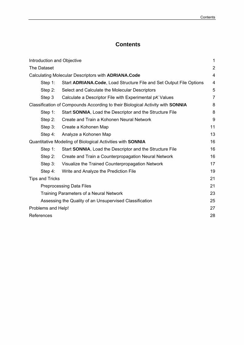
Contents

Contents

Introduction and Objective 1 The Dataset 2 Calculating Molecular Descriptors with ADRIANA.Code 4

Step 1: Start ADRIANA.Code, Load Structure File and Set Output File Options 4 Step 2: Select and Calculate the Molecular Descriptors 5 Step 3 Calculate a Descriptor File with Experimental pK Values 7

Classification of Compounds According to their Biological Activity with SONNIA 8 Step 1: Start SONNIA, Load the Descriptor and the Structure File 8 Step 2: Create and Train a Kohonen Neural Network 9 Step 3: Create a Kohonen Map 11 Step 4: Analyze a Kohonen Map 13

Quantitative Modeling of Biological Activities with SONNIA 16 Step 1: Start SONNIA, Load the Descriptor and the Structure File 16 Step 2: Create and Train a Counterpropagation Neural Network 16 Step 3: Visualize the Trained Counterpropagation Network 17 Step 4: Write and Analyze the Prediction File 19

Tips and Tricks 21 Preprocessing Data Files 21 Training Parameters of a Neural Network 23 Assessing the Quality of an Unsupervised Classification 25

Problems and Help! 27 References 28

Introduction and Objective

1

Introduction and Objective

Statistical or machine learning methods are widely used to establish relationships between biological activities, physical or chemical properties of a compound and its chemical structure. These methods, in combination with structure descriptors, are used to derive models that can be applied to predict properties of new compounds.

The objective of this tutorial is to show on an example how the methods

• descriptor calculation package ADRIANA.Code [1], and

• neural network package SONNIA [2]

can be applied in the area of qualitative and quantitative structure-activity relationship (QSAR) studies. The tutorial guides the user through the entire workflow starting from a dataset of chemical structures with experimentally derived biological activities and describes

• how to calculate molecular descriptors for a dataset of compounds with ADRIANA.Code,

• how to classify compounds according to their biological activity with a Kohonen neural network implemented in SONNIA, and

• how to quantitatively model a biological activity using the counterpropagation neural network implemented in SONNIA.

In addition, the tutorial gives some hints, tips and tricks that are valuable and helpful when ADRIANA.Code and SONNIA are applied to other datasets and in QSAR studies.

For further information about the usage as well as the methods that are implemented in the program packages ADRIANA.Code and SONNIA, please refer to the respective program manuals.

The example "Modeling Corticosteroid Binding Globulin (CBG) Receptor Activity" is taken from the literature [3]. The dataset comprises 31 steroid compounds and their experimental CBG receptor binding affinity values (pK values). Based on the pK values, the compounds were pre-classified into the three different classes, high, medium and low CBG binding affinity. In the example study, each molecule of the dataset is represented by a vector of 12 autocorrelation coefficients that encode the spatial distribution of the electrostatic potential on the molecular surface (calculated by ADRIANA.Code). These descriptors are then used to classify the compounds according to the three different CBG activity classes using an unsupervised Kohonen neural network technique (implemented in SONNIA). Finally, a supervised neural network method (counterpropagation neural network implemented in SONNIA) is used to quantitatively model the pK values.

The dataset of 31 steroid compounds can be downloaded from Molecular Networks' web server at http://www.molecular-networks.com.

The Dataset

2

The Dataset

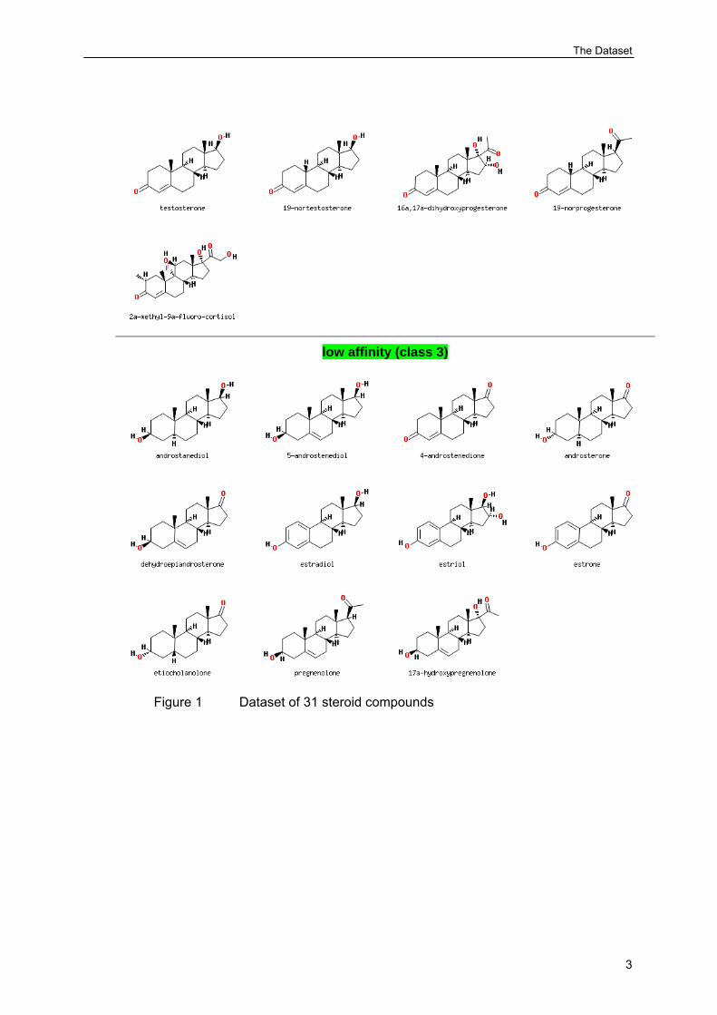
The dataset of 31 steroid compounds and their CBG receptor binding affinity values are stored in MDL SDFile format [4]. All chemical structures are fully defined including hydrogen atoms and stereo information (atom parity flags). For each record, the experimentally determined biological activity (pK value) is contained in the SDF data field <CBG_ACTIVITY_pK>. Furthermore, the compounds are pre-classified into three different affinity classes:

high affinity (class 1) medium affinity (class 2) low affinity (class 3)

The binding affinity class is stored in the SDF data field <CBG_ACTIVITY_CLASS>. Figure 1 shows the structures of the dataset sorted by their CBG receptor binding affinity class.

high affinity (class 1)

medium affinity (class 2)

The Dataset

3

low affinity (class 3)

Figure 1 Dataset of 31 steroid compounds

Calculating Molecular Descriptors with ADRIANA.Code

4


In the following sections, the calculation of a set of molecular descriptors with ADRIANA.Code is described. A descriptor file will be generated that represents each molecule of the dataset by a vector of 12 autocorrelation coefficients encoding the spatial distribution of the electrostatic potential on the molecular surface.

Step 1: Start ADRIANA.Code, Load Structure File and Set Output File Options

• Start the graphical user interface (GUI) of ADRIANA.Code by double-clicking on the desktop icon of ADRIANA.Code.

• Load the structure file steroids31_act.sdf by clicking on the button ... in the section Input of the ADRIANA.Code GUI and selecting the file in the dialog box Choose a structure file to open (see Figure 2).

Figure 2 Loading a chemical structure file.

• Set the output file format in the drop down menu Format in the section Output to SONNIA.

• Click on the button ... in the section Output and set the name of the output file to steroids31_actClass_mep_ac12.dat in the same directory where the input file is located in the dialog box Choose an output file to write to.


5

• Note: The full name of the output file (file name and path) is set automatically but can be changed by the user either in the field File in the section Output or by using the dialog box as described above.

• Click on the button Select properties in the section Output, choose NAME in the drop down menu Compound ID property, check the box CBG_ACTIVITY_CLASS in the list Select properties to copy and confirm with the button OK (see Figure 3).

Figure 3 Selecting the properties of the output file.

Step 2: Select and Calculate the Molecular Descriptors

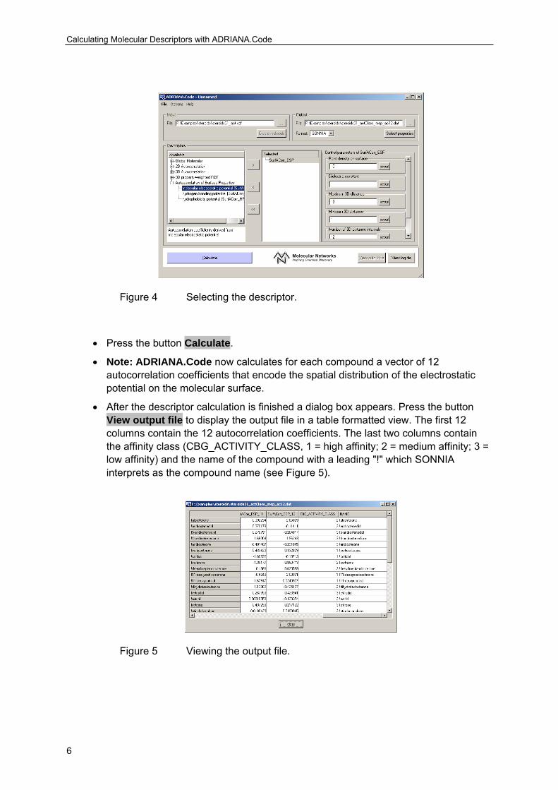
• Select Autocorrelation of Molecular Surface Properties → molecular electrostatic potential (SurfACorr_ESP) in the list Available in the section Descriptors and press the button > to select the descriptor for calculation.

• SurfACorr_ESP now appears in the list Selected. Use the default settings and parameters in the section Available Control Parameters (see Figure 4).


6

Figure 4 Selecting the descriptor.

• Press the button Calculate.

• Note: ADRIANA.Code now calculates for each compound a vector of 12 autocorrelation coefficients that encode the spatial distribution of the electrostatic potential on the molecular surface.

• After the descriptor calculation is finished a dialog box appears. Press the button View output file to display the output file in a table formatted view. The first 12 columns contain the 12 autocorrelation coefficients. The last two columns contain the affinity class (CBG_ACTIVITY_CLASS, 1 = high affinity; 2 = medium affinity; 3 = low affinity) and the name of the compound with a leading "!" which SONNIA interprets as the compound name (see Figure 5).

Figure 5 Viewing the output file.


7

Step 3 Calculate a Descriptor File with Experimental pK Values

• Change the name of the output file to steroids31_actpK_mep_ac12.dat.

• Select CBG_ACTIVITY_pK in the dialog box Select properties instead of CBG_ACTIVITY_CLASS and confirm with the button OK (see Figure 6).

Figure 6 Selecting the properties of the output file.

• Calculate the descriptors by pressing the button Calculate.

Classification of Compounds According to their Biological Activity with SONNIA

8


The following section describes the classification of the steroid compounds according to their CBG binding affinity class (CBG_ACTIVITY_CLASS) using the Kohonen neural network algorithm implemented in SONNIA. The Kohonen algorithm is an unsupervised, non-linear mapping technique that projects the twelve-dimensional descriptor space (12 autocorrelation coefficients) into a two-dimensional plane (Kohonen map). The information about the CBG affinity class is not used for the projection (unsupervised learning). The neurons of the resulting Kohonen map are color-coded according to the CBG receptor binding affinity class (high, medium or low) of the compounds that are assigned to a specific neuron.

Step 1: Start SONNIA, Load the Descriptor and the Structure File

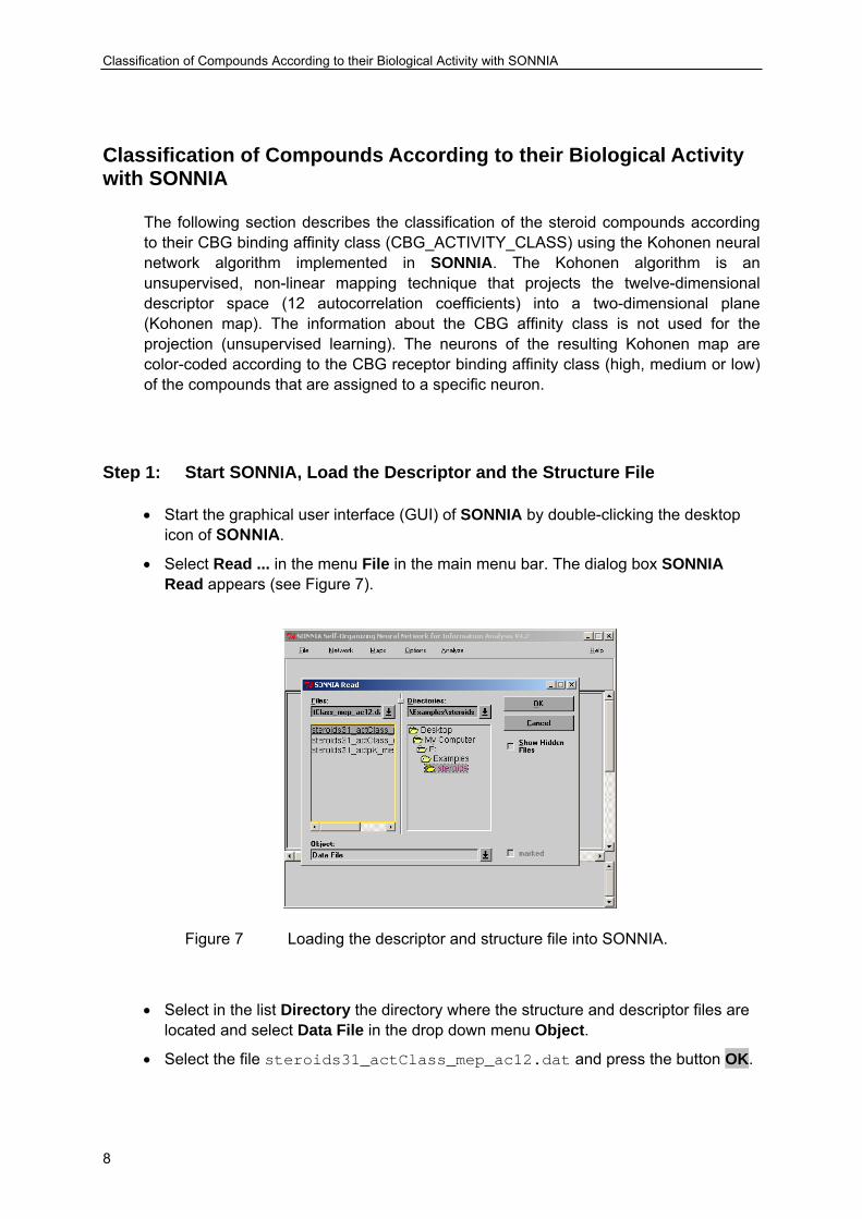
• Start the graphical user interface (GUI) of SONNIA by double-clicking the desktop icon of SONNIA.

• Select Read ... in the menu File in the main menu bar. The dialog box SONNIA Read appears (see Figure 7).

Figure 7 Loading the descriptor and structure file into SONNIA.

• Select in the list Directory the directory where the structure and descriptor files are located and select Data File in the drop down menu Object.

• Select the file steroids31_actClass_mep_ac12.dat and press the button OK.


9

• In order to load the structure file, repeat this procedure, but select Structure File in the drop down menu Object and select the file steroids31_act.sdf.

Step 2: Create and Train a Kohonen Neural Network

• Select Create ... in the menu Network in the main menu bar. The dialog box SONNIA Network appears (see Figure 8).

Figure 8 Creating a Kohonen neural network.

• Ensure that Kohonen is set in the drop-down menu in the section Algorithm and Topology is set to toroidal.

• The size of the network is set automatically by SONNIA. In this example, the network has a size of 5 (width) x 3 (height) = 15 neurons.

• Enter the number 12 in the field Input in the section Network Dimensions (this is the number of descriptors of each molecule). Use the default settings for all other parameters. In this case the network (plane) has a dimension of 5 (width) x 3 (height) = 15 neurons. Press the button Create.

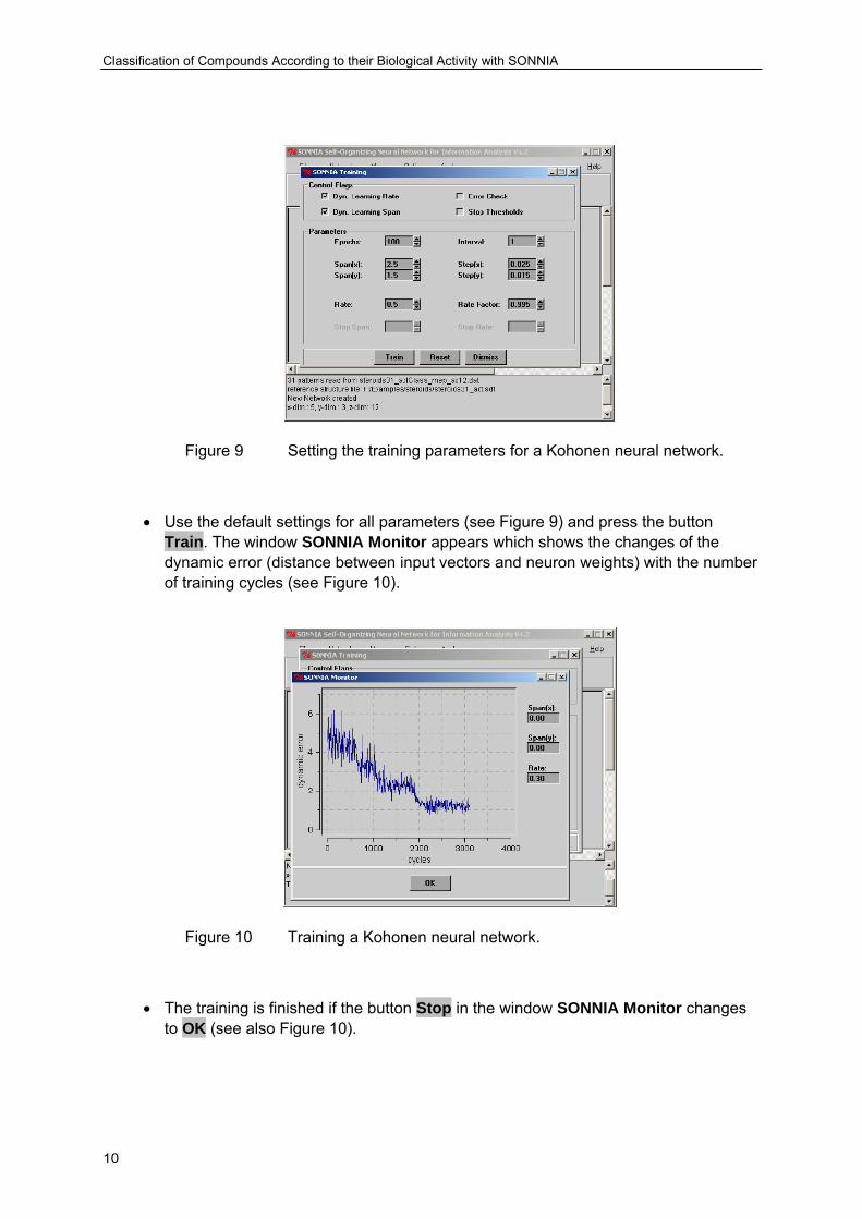
• Select Train ... in the menu Network in the main menu bar. The dialog box SONNIA Training appears (see Figure 9).


10

Figure 9 Setting the training parameters for a Kohonen neural network.

• Use the default settings for all parameters (see Figure 9) and press the button Train. The window SONNIA Monitor appears which shows the changes of the dynamic error (distance between input vectors and neuron weights) with the number of training cycles (see Figure 10).

Figure 10 Training a Kohonen neural network.

• The training is finished if the button Stop in the window SONNIA Monitor changes to OK (see also Figure 10).


11

Step 3: Create a Kohonen Map

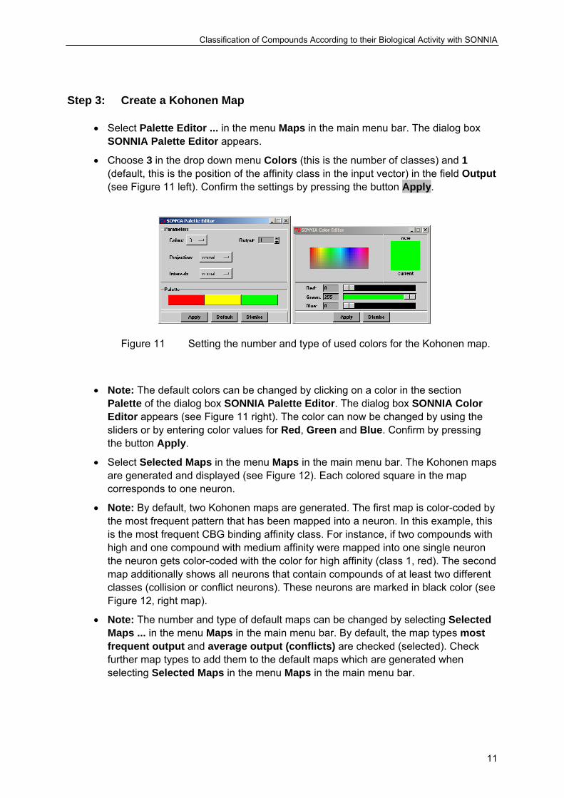
• Select Palette Editor ... in the menu Maps in the main menu bar. The dialog box SONNIA Palette Editor appears.

• Choose 3 in the drop down menu Colors (this is the number of classes) and 1 (default, this is the position of the affinity class in the input vector) in the field Output (see Figure 11 left). Confirm the settings by pressing the button Apply.

Figure 11 Setting the number and type of used colors for the Kohonen map.

• Note: The default colors can be changed by clicking on a color in the section Palette of the dialog box SONNIA Palette Editor. The dialog box SONNIA Color Editor appears (see Figure 11 right). The color can now be changed by using the sliders or by entering color values for Red, Green and Blue. Confirm by pressing the button Apply.

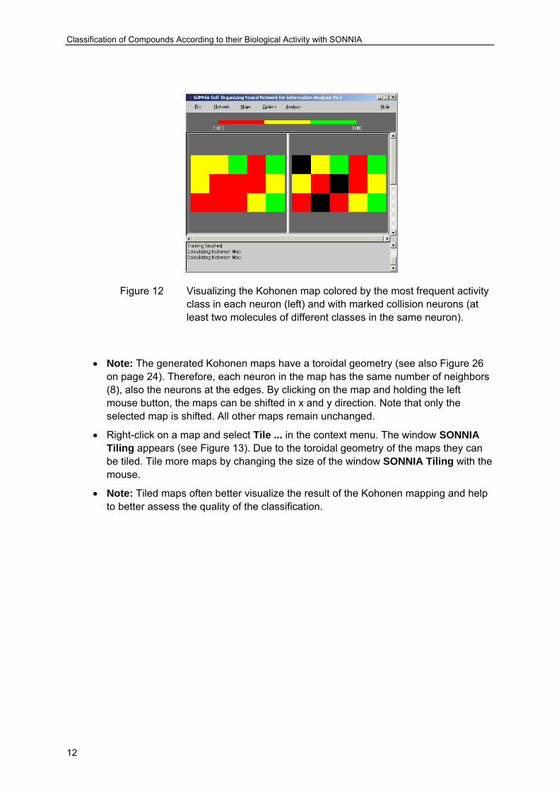
• Select Selected Maps in the menu Maps in the main menu bar. The Kohonen maps are generated and displayed (see Figure 12). Each colored square in the map corresponds to one neuron.

• Note: By default, two Kohonen maps are generated. The first map is color-coded by the most frequent pattern that has been mapped into a neuron. In this example, this is the most frequent CBG binding affinity class. For instance, if two compounds with high and one compound with medium affinity were mapped into one single neuron the neuron gets color-coded with the color for high affinity (class 1, red). The second map additionally shows all neurons that contain compounds of at least two different classes (collision or conflict neurons). These neurons are marked in black color (see Figure 12, right map).

• Note: The number and type of default maps can be changed by selecting Selected Maps ... in the menu Maps in the main menu bar. By default, the map types most frequent output and average output (conflicts) are checked (selected). Check further map types to add them to the default maps which are generated when selecting Selected Maps in the menu Maps in the main menu bar.


12

Figure 12 Visualizing the Kohonen map colored by the most frequent activity class in each neuron (left) and with marked collision neurons (at least two molecules of different classes in the same neuron).

• Note: The generated Kohonen maps have a toroidal geometry (see also Figure 26 on page 24). Therefore, each neuron in the map has the same number of neighbors (8), also the neurons at the edges. By clicking on the map and holding the left mouse button, the maps can be shifted in x and y direction. Note that only the selected map is shifted. All other maps remain unchanged.

• Right-click on a map and select Tile ... in the context menu. The window SONNIA Tiling appears (see Figure 13). Due to the toroidal geometry of the maps they can be tiled. Tile more maps by changing the size of the window SONNIA Tiling with the mouse.

• Note: Tiled maps often better visualize the result of the Kohonen mapping and help to better assess the quality of the classification.


13

Figure 13 Tiling of a Kohonen map.

Step 4: Analyze a Kohonen Map

• In order to visualize which compounds were mapped into which neurons, left-click on a neuron while keeping the Crtl key pressed. The neuron is now selected and is marked in light-grey color.

• Right-click on the selected neuron and select Export Structures ... in the context menu. The Structure Browser appears and displays the compounds that have been mapped into the selected neurons (see Figure 14).

Figure 14 Displaying the chemical structures that are mapped to a specific neuron.


14

• Note: The structure file must have been loaded into SONNIA (see also Figure 7) to use this functionality.

• Note: More than one neuron can be selected by a left-click on the map while keeping the Crtl key pressed and dragging the mouse over the map. The focus of the selection is shown by a temporary rectangle while dragging the mouse. All selected neurons are finally marked in light-gray color.

• Note: Neurons can be de-selected by left-clicking on the neuron while keeping the Crtl and the Shift key pressed.

• Note: Additional properties that are stored in the structure file (e.g., compound names, CBG affinity classes) can be displayed in the Structure Browser by selecting Chemical Properties ... in the menu Display of the main menu bar of the structure browser (Prop tabs in the Browser Annotation Display Style).

• Right-click on a map and select Export Centroids ... in the context menu. The Structure Browser appears. The browser now displays the centroid compounds of all neurons (see Figure 15). The arrangement of the structure browser always reproduces the size of the network (here: 5 x 3).

• Note: The centroid compound of a neuron is the compound having a descriptor vector (twelve dimensions) most similar to the weights of the neuron vector (also twelve dimensions). The descriptor vector of the centroid compound has the minimum Euclidean distance to the vector of the neuron weights of all compounds that have been mapped to this neuron.

Figure 15 Displaying the centroid structures of all neurons.

• In order to export the contents of all neurons (i.e., the information which compounds are mapped into which neurons), select Export Contents ... in the menu Analyze in the main menu bar. The dialog box SONNIA Write appears (see Figure 16).


15

Figure 16 Exporting the contents of all neurons.

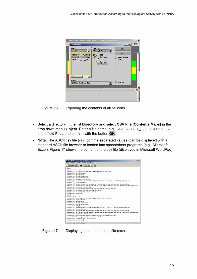
• Select a directory in the list Directory and select CSV File (Contents Maps) in the drop down menu Object. Enter a file name, e.g., steroids31_contentMap.csv, in the field Files and confirm with the button OK.

• Note: The ASCII csv file (csv: comma separated values) can be displayed with a standard ASCII file browser or loaded into spreadsheet programs (e.g., Microsoft Excel). Figure 17 shows the content of the csv file (displayed in Microsoft WordPad).

Figure 17 Displaying a contents maps file (csv).

Quantitative Modeling of Biological Activities with SONNIA

16


The following section describes the quantitative modeling of the CBG receptor binding affinity (CBG_ACTIVITY_pK) of the 31 steroid compounds using the counterpropagation neural network algorithm implemented in SONNIA. Again, each compound of the dataset is represented by a twelve-dimensional autocorrelation vector that encodes the spatial distribution of the electrostatic potential on the molecular surface. The counterpropagation algorithm is a supervised learning technique. In contrast to the Kohonen algorithm, the pK values of the CBG receptor binding affinity are now used to derive a model expressing the relationship between the descriptors (independent variables) and the biological activity (dependent variables).

Step 1: Start SONNIA, Load the Descriptor and the Structure File

• Start the graphical user interface (GUI) of SONNIA by double-clicking the desktop icon.

• Select Read ... in the menu File in the main menu bar. The dialog box SONNIA Read appears (see also Figure 7).

• Select in the list Directory the directory where the structure and descriptor files are located and select Data File in the drop down menu Object.

• Select the file steroids31_actpK_mep_ac12.dat and press the button OK.

• In order to load the structure file, repeat this procedure, but select Structure File in the drop down menu Object and select the file steroids31_act.sdf.

Step 2: Create and Train a Counterpropagation Neural Network

• Select Create ... in the menu Network in the main menu bar. The dialog box SONNIA Network appears (see Figure 18).


17

Figure 18 Creating a counterpropagation network.

• Select Counterprop. in the drop down menu of the section Algorithm. Ensure that Topology is set to toroidal.

• Enter the number 12 (dimension of descriptor vector) in the field Input and 1 in the field Output (dimension of the property to model, single value of CBG binding affinity) in the section Network Dimensions. Use the default settings for all other parameters and press the button Create.

• Select Train ... in the menu Network in the main menu bar. The dialog box SONNIA Training appears (see also Figure 9).

• Use the default settings for all parameters and press the button Train. The window SONNIA Monitor appears which shows the changes of the dynamic error (distance between input vectors and neuron weights) with the number of training cycles (see also Figure 10).

• The training is finished when the button Stop in the window SONNIA Monitor changes to OK (see also Figure 10).

Step 3: Visualize the Trained Counterpropagation Network

• Note: The trained counterpropagation network can be visualized in a style similar to a Kohonen map. In this example, a continuous value (pK value) is modeled which ranges from about -7.8 to -5.0. The number of colors that are available in SONNIA is limited to 10. Therefore, only ranges of the predicted values can be color-coded by a single color.


18

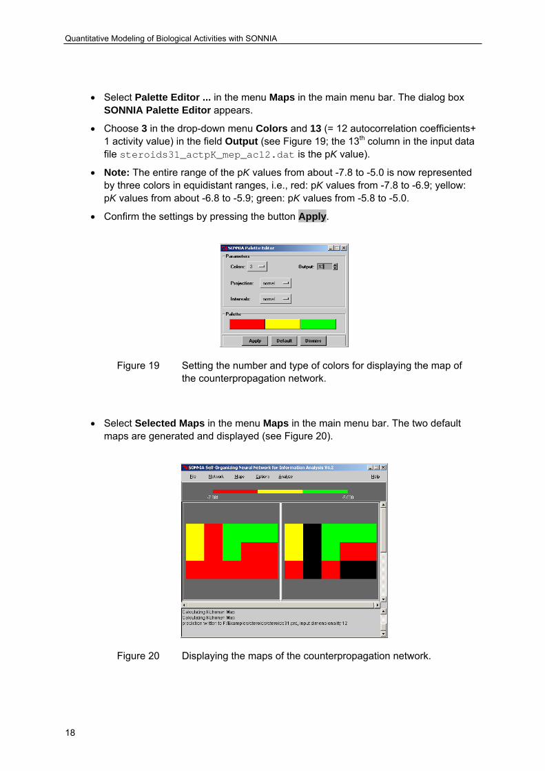
• Select Palette Editor ... in the menu Maps in the main menu bar. The dialog box SONNIA Palette Editor appears.

• Choose 3 in the drop-down menu Colors and 13 (= 12 autocorrelation coefficients+ 1 activity value) in the field Output (see Figure 19; the 13th column in the input data file steroids31_actpK_mep_ac12.dat is the pK value).

• Note: The entire range of the pK values from about -7.8 to -5.0 is now represented by three colors in equidistant ranges, i.e., red: pK values from -7.8 to -6.9; yellow: pK values from about -6.8 to -5.9; green: pK values from -5.8 to -5.0.

• Confirm the settings by pressing the button Apply.

Figure 19 Setting the number and type of colors for displaying the map of the counterpropagation network.

• Select Selected Maps in the menu Maps in the main menu bar. The two default maps are generated and displayed (see Figure 20).

Figure 20 Displaying the maps of the counterpropagation network.


19

Step 4: Write and Analyze the Prediction File

• In order to write out the predicted pK values by the counterpropagation network select Write in the menu File in the main menu bar. The dialog box SONNIA Write appears (see Figure 21).

• Select Prediction File in the drop down menu Object and enter a file name in the field Files (e.g., steroids31.prd).

• Confirm with the button OK. The dialog box Prediction appears and suggests in the field Input Dimensionality the figure 12 (see Figure 21; number of descriptors of each compound). Confirm with the button Apply.

Figure 21 Writing the prediction file.

• Note: The prediction file steroids31.prd is an ASCII file which lists the input Y variable(s) (experimental pK values), the predicted Y variable(s) (predicted pK values) and the name of the compound. The file can be loaded in spreadsheet applications or standard ASCII text browser for further analysis (see Figure 22 and Figure 23).


20

Figure 22 Loading a prediction file into a spreadsheet application (here: MS Excel).

Figure 23 Analyzing the prediction of SONNIA (here: MS Excel).

Tips and Tricks

21

Tips and Tricks

Preprocessing Data Files

Merging Structure and Property Data

Often, the chemical structure data is stored in an MDL SDFile whereas any additional information related to the chemical structures (e.g., any measured or experimental data) is stored in a separate file, e.g., in a table-like formatted ASCII file. A primary key (e.g., a unique name or number of the chemical structures) that is present in both the SD and the ASCII file is the only link between the structure and the additional data.

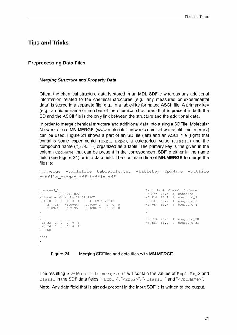
In order to merge chemical structure and additional data into a single SDFile, Molecular Networks' tool MN.MERGE (www.molecular-networks.com/software/split_join_merge/) can be used. Figure 24 shows a part of an SDFile (left) and an ASCII file (right) that contains some experimental (Exp1, Exp2), a categorical value (Class1) and the compound name (CpdName) organized as a table. The primary key is the given in the column CpdName that can be present in the correspondent SDFile either in the name field (see Figure 24) or in a data field. The command line of MN.MERGE to merge the files is:

mn.merge –tablefile tablefile.txt –tablekey CpdName –outfile outfile_merged.sdf infile.sdf

compound_1 CS 02280711002D 0 Molecular Networks 28.02.2007 54 58 0 0 0 0 0 0 0 0999 V2000 2.8729 -2.0044 0.0000 C 0 0 0 2.8920 -0.9195 0.0000 C 0 0 0 . . . 25 33 1 0 0 0 0 26 34 1 0 0 0 0 M END $$$$ . .

Exp1 Exp2 Class1 CpdName -6.279 71.5 2 compound_1 -5.316 63.4 3 compound_2 -5.334 69.7 3 compound_3 -5.763 65.7 3 compound_4 . . . -5.613 79.5 3 compound_30 -7.881 69.0 1 compound_31

Figure 24 Merging SDFiles and data files with MN.MERGE.

The resulting SDFile outfile_merge.sdf will contain the values of Exp1, Exp2 and Class1 in the SDF data fields "<Exp1>", "<Exp2>", "<Class1>" and "<CpdName>".

Note: Any data field that is already present in the input SDFile is written to the output.

Tips and Tricks

22

Standardization and Checking Structural State and Integrity of Structure Files

Chemical structure files may originate from different sources. Therefore, the chemical structures may differ in the way they are coded in their connection table representation or even show some errors. For instance, functional groups such as nitro groups may be coded with a pentavalent nitrogen atom or as a charged species, hydrogen atoms may be given implicitly or explicitly or charges in salts may not be balanced correctly. However, for a corporate compound database or a dataset under investigation it may be mandatory that all chemical structures and their connection table representation comply with a certain standard, i.e., are coded in a consistent and pre-defined fashion.

Molecular Networks' tool MN.CHECK (www.molecular-networks.com/software/check/) can be helpful to standardize chemical structure data by applying a set of business rules that can be selected by the user. MN.CHECK supports batch mode execution and is able to process large chemical files fast and efficient. Furthermore, MN.CHECK can be used to detect and correct errors in the structure coding (e.g., missing charges at counter ions in salts) and to identify and remove duplicate structures in large collections of chemical compounds (based on a 64bit hashcoding technique).

For example, the MN.CHECK command line

mn.check -hydrogen add -nitrostyle ionic -chargebalance -pedantic -unique -outfile outfile_checked.sdf infile.sdf

will read in the file infile.sdf, add implicit hydrogen atoms, re-code all nitro groups (and similar functional units) as charge pairs (with a tetravalent, positively charged nitrogen atom, and a negatively charged oxygen atom or another ligand atom), balance charges in salts, pedantically check the file formatting and structure coding and write out a message when errors are detected, identify and remove duplicate structures and write out the normalized and checked structures to the file outfile_checked.sdf.

Complementary Software

Another helpful and valuable tool in this area is Molecular Networks' file format converter MN.CONVERT that supports over 50 different file formats for chemical structure and reaction information and interconverts them with high conversion rates and reliability. A complete list of all supported file formats can be found at the product page of MN.CONVERT at www.molecular-networks.com/software/convert/.

2D structure diagrams (2D coordinates) in publishing quality can be generated with Molecular Networks' tool MN.2DCOOR. The tool offers a variety of options and features to customize the layout of 2D structure plots. For instance, structures can be aligned to their main x or y axes or to a template structure provided in a separate file (e.g., to align all structures in a combinatorial library to a predefined orientation of their common scaffold). Further information about MN.2DCOOR can be found at its product page at www.molecular-networks.com/software/2dcoor.

Tips and Tricks

23

Training Parameters of a Neural Network

Network Size

By default, SONNIA suggests a ratio of approximately one neuron per two compounds/patterns (1:2) which usually works fine for initial tests. Another possibility is to start with a ratio of 1:1 and to gradually reduce the size in following runs. If the size of the network gets too large there is a high likelihood that it will only memorize the input data without showing the maximum of the actual neighborhood relationship of the data patterns (e.g., by conflict neurons, neurons with patterns of more than one class, e.g., known actives and unknown).

Smaller networks (high neuron/pattern ratio) tend to produce more conflict neurons which might be of interest for some applications, e.g., for lead-hopping. However, in too small networks the data has to be compressed in a few neurons. This may lead to conflict neurons that are not very meaningful. A balanced ratio should be achieved. Another example for a rather high neuron/pattern ratio is the visualization of large chemical spaces. Figure 25 shows the projection of about 404,000 chemical compounds from different sources into a Kohonen map of the size 80 x 60 neurons.

# of compounds: 404,449# of neurons: 4,800 (80 x 60)# of occupied neurons: 4,799

Chemical supplierdatabases (139,961)

NCI database (193,339)

MDDR (71,149)

Color coding: most frequentpattern in neuron, scaled

Figure 25 Visualization of large chemical spaces with SONNIA.

Network Topology

SONNIA offers two different types of network topology, a toroidal and a rectangular topology

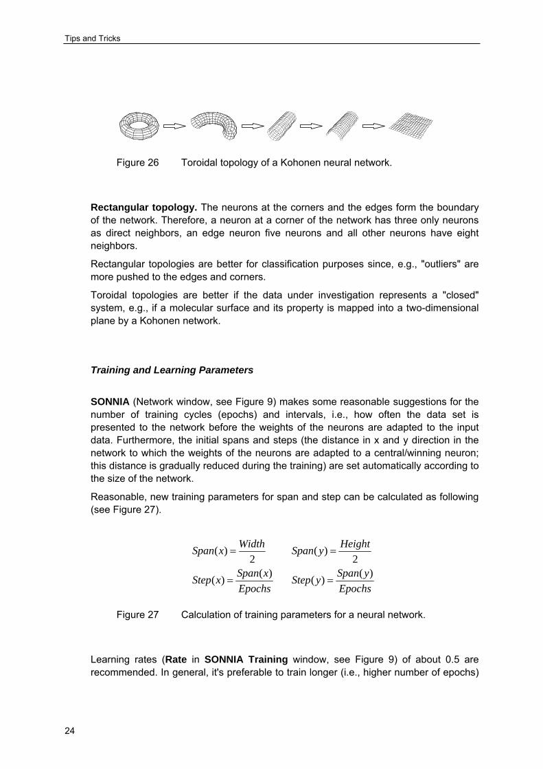
Toroidal topology. All neurons have the same neighbor relationship, i.e., eight direct neighbors. This means that in the resulting Kohonen map the neurons at the corners and edges are adjacent to the neurons at the opposite site of the map. This can be illustrated by a torus that is cut two times to obtain a plane (see Figure 26).

Tips and Tricks

24

Figure 26 Toroidal topology of a Kohonen neural network.

Rectangular topology. The neurons at the corners and the edges form the boundary of the network. Therefore, a neuron at a corner of the network has three only neurons as direct neighbors, an edge neuron five neurons and all other neurons have eight neighbors.

Rectangular topologies are better for classification purposes since, e.g., "outliers" are more pushed to the edges and corners.

Toroidal topologies are better if the data under investigation represents a "closed" system, e.g., if a molecular surface and its property is mapped into a two-dimensional plane by a Kohonen network.

Training and Learning Parameters

SONNIA (Network window, see Figure 9) makes some reasonable suggestions for the number of training cycles (epochs) and intervals, i.e., how often the data set is presented to the network before the weights of the neurons are adapted to the input data. Furthermore, the initial spans and steps (the distance in x and y direction in the network to which the weights of the neurons are adapted to a central/winning neuron; this distance is gradually reduced during the training) are set automatically according to the size of the network.

Reasonable, new training parameters for span and step can be calculated as following (see Figure 27).

EpochsySpanyStep

EpochsxSpanxStep

HeightySpanWidthxSpan

)()()()(

2)(

2)(

==

==

Figure 27 Calculation of training parameters for a neural network.

Learning rates (Rate in SONNIA Training window, see Figure 9) of about 0.5 are recommended. In general, it's preferable to train longer (i.e., higher number of epochs)

Tips and Tricks

25

but with lower learning rates. High learning rates may cause problems if several input patterns compete for one neuron.

The rate factor (Rate Factor in SONNIA Training window, see Figure 9) reduces the learning rate after each epoch by multiplying the learning rate with the rate factor. At the beginning of the training

In general, Kohonen (or SOM) mapping is quite powerful since you can very quickly do a visual inspection of a high dimensional space and it allows for a rapid assessment and evaluation if the used descriptors are able to reveal trends and patterns in the data.

Assessing the Quality of an Unsupervised Classification

Basically, there are three different criteria which can be used to assess the quality of a classification done by a Kohonen mapping. These three criteria, visual inspection, occupancy and number of collisions (conflict neurons) are described in the following. Note that all three criteria should be taken into account to support the decision whether a generated Kohonen map shows a "good" classification.

Visual Inspection

The strength of Kohonen maps is that they can be generated rather quickly and the results can be visually inspected. The visual inspection allows for a rapid assessment and evaluation if the used descriptors are able to reveal trends and patterns in the data ("... human inspection building on the powerful pattern recognition capabilities of the human mind") [7].

A Kohonen map that shows a clear separation of different classes of compounds in a dataset can be regarded as an indicator that there is a relationship between the used descriptor(s) and the property under investigation.

Occupancy

A well-trained Kohonen network should also show a balanced and even distribution of the patterns (i.e., compounds) over the resulting map as well as a low fraction of unoccupied neurons (shown as white squares in the map). The distribution of the patterns and the occupancy of each individual neuron can be checked with an "occupancy map" (menu Maps in the main menu bar of SONNIA, see Figure 28, right map). The occupancy map is color-coded by the number of patterns/compounds that are assigned to each neurons.

Tips and Tricks

26

Figure 28 Occupancy map of a Kohonen neural network (right map).

A Kohonen map with an unbalanced occupancy of the neurons (e.g., more than the half of the input patterns are located in only 10% of the total number of neurons) may have several reasons, e.g.,

• The training of the network was stopped too early: Train a newly created network and increase the number of Epochs (adjust the values for Step(x) and Step(y) accordingly).

• The input values of one or a few input patterns are rather different from the rest of the input patterns of the dataset ("outliers"): remove these patterns from your training set and train a newly created network with the reduced dataset.

Problems and Help!

27

Problems and Help!

If there are any difficulties with the installation of ADRIANA.Code or SONNIA or if any problems occur while running ADRIANA.Code or SONNIA please send all inquiries to the following address:

Molecular Networks GmbH Computerchemie Henkestr. 91 91052 Erlangen Germany or contact us by email [email protected]

or by Fax +49-9131-815669

References

28

References

[1] Descriptor Calculation Package ADRIANA.Code, developed and distributed by Molecular Networks GmbH, Erlangen, Germany (http://www.molecular-networks.com).

[2] Neural Networks Package SONNIA, developed and distributed by Molecular Networks GmbH, Erlangen, Germany (http://www.molecular-networks.com).

[3] Wagener, M.; Sadowski, J.; Gasteiger, J. Autocorrelation of Molecular Surface Properties for Modeling Corticosteroid Binding Globulin and Cytosolic Ah Receptor Activity by Neural Networks. J. Am. Chem. Soc. 1995, 117, 7769-7775.

[4] a) Dalby, A.; Nourse, J. G.; Hounshell, W. D.; Gushurst, A. K. I.; Grier, D. L.; Leland, B. A.; Laufer, J. Description of Several Chemical Structure File Formats Used by Computer Programs Developed at Molecular Design Limited. J. Chem. Inf. Comput. Sci. 1992, 32, 244-255. b) A detailed description of MDL file formats (Mol, SDF and RDF) is available for download as a PDF document at http://www.mdli.com.

[5] Sadowski, J.; Gasteiger, J.; Klebe, G. Comparison of Automatic Three-Dimensional Model Builders Using 639 X-Ray Structures. J. Chem. Inf. Comput. Sci. 1994, 34, 1000-1008.

[6] 3D Structure Generator CORINA, developed and distributed by Molecular Networks GmbH, Erlangen, Germany (http://www.molecular-networks.com).

[7] Zupan, J.; Gasteiger, J. Neural Network in Chemistry and Drug Design. Second Edition, Wiley-VCH, Weinheim, 1999, 380 pages, ISBN 3-527-29778-2.

and SONNIA Tutorial - Molecular Networks

Documents

Transcript of and SONNIA Tutorial - Molecular Networks