- · PDF filemembers of the structures. ... L.S. Negi & R.S. Jangid, Tata McGraw-Hill...
319
www.Vidyarthiplus.com www.Vidyarthiplus.com Page 1 CE2302 STRUCTURAL ANALYSIS – CLASSICAL METHODS 3 1 0 4 OBJECTIVE The members of a structure are subjected to internal forces like axial forces, shearing forces, bending and torsional moments while transferring the loads acting on it. Structural analysis deals with analysing these internal forces in the members of the structures. At the end of this course students will be conversant with classical method of analysis. UNIT I DEFLECTION OF DETERMINATE STRUCTURES 9 Principles of virtual work for deflections – Deflections of pin-jointed plane frames and rigid plane frames – Willot diagram - Mohr’s correction UNIT II MOVING LOADS AND INFLUENCE LINES 9 (DETERMINATE & INDETERMINATE STRUCTURES) Influence lines for reactions in statically determinate structures – influence lines for members forces in pin-jointed frames – Influence lines for shear force and bending moment in beam sections – Calculation of critical stress resultants due to concentrated and distributed moving loads. Muller Breslau’s principle – Influence lines for continuous beams and single storey rigid frames – Indirect model analysis for influence lines of indeterminate structures – Beggs deformeter UNIT III ARCHES 9 Arches as structural forms – Examples of arch structures – Types of arches – Analysis of three hinged, two hinged and fixed arches, parabolic and circular arches – Settlement and temperature effects. UNIT IV SLOPE DEFLECTION METHOD 9 Continuous beams and rigid frames (with and without sway) – Symmetry and antisymmetry – Simplification for hinged end – Support displacements. UNIT V MOMENT DISTRIBUTION METHOD 9 Distribution and carry over of moments – Stiffness and carry over factors – Analysis of continuous beams – Plane rigid frames with and without sway – Naylor’s simplification. TUTORIAL 15 TOTAL : 60 TEXT BOOKS 1. “Comprehensive Structural Analysis – Vol. 1 & Vol. 2”, Vaidyanadhan, R and Perumal, P, Laxmi Publications, New Delhi, 2003 2. “Structural Analysis”, L.S. Negi & R.S. Jangid, Tata McGraw-Hill Publications, New Delhi, Sixth Edition, 2003 3. Punmia B.C., Theory of Structures (SMTS ) Vol II laxmi Publishing Pvt ltd, New Delhi, 2004 REFERENCES 1. Analysis of Indeterminate Structures – C.K. Wang, Tata McGraw-Hill, 1992 Comment [R2]: Comment [R1]:
Transcript of - · PDF filemembers of the structures. ... L.S. Negi & R.S. Jangid, Tata McGraw-Hill...

www.Vidyarthiplus.com
www.Vidyarthiplus.com Page 1
CE2302 STRUCTURAL ANALYSIS – CLASSICAL METHODS 3 1 0 4 OBJECTIVE
The members of a structure are subjected to internal forces like axial forces, shearing forces, bending and torsional moments while transferring the loads acting on it. Structural analysis deals with analysing these internal forces in the members of the structures. At the end of this course students will be conversant with classical method of analysis. UNIT I DEFLECTION OF DETERMINATE STRUCTURES 9
Principles of virtual work for deflections – Deflections of pin-jointed plane frames and rigid plane frames – Willot diagram - Mohr’s correction
UNIT II MOVING LOADS AND INFLUENCE LINES 9 (DETERMINATE & INDETERMINATE STRUCTURES)
Influence lines for reactions in statically determinate structures – influence lines for members forces in pin-jointed frames – Influence lines for shear force and bending moment in beam sections – Calculation of critical stress resultants due to concentrated and distributed moving loads.
Muller Breslau’s principle – Influence lines for continuous beams and single storey rigid frames – Indirect model analysis for influence lines of indeterminate structures – Beggs deformeter UNIT III ARCHES 9
Arches as structural forms – Examples of arch structures – Types of arches – Analysis of three hinged, two hinged and fixed arches, parabolic and circular arches – Settlement and temperature effects.
UNIT IV SLOPE DEFLECTION METHOD 9
Continuous beams and rigid frames (with and without sway) – Symmetry and antisymmetry – Simplification for hinged end – Support displacements.
UNIT V MOMENT DISTRIBUTION METHOD 9
Distribution and carry over of moments – Stiffness and carry over factors – Analysis of continuous beams – Plane rigid frames with and without sway – Naylor’s simplification.
TUTORIAL 15 TOTAL : 60
TEXT BOOKS
1. “Comprehensive Structural Analysis – Vol. 1 & Vol. 2”, Vaidyanadhan, R and Perumal, P, Laxmi Publications, New Delhi, 2003
2. “Structural Analysis”, L.S. Negi & R.S. Jangid, Tata McGraw-Hill Publications, New Delhi, Sixth Edition, 2003
3. Punmia B.C., Theory of Structures (SMTS ) Vol II laxmi Publishing Pvt ltd, New Delhi, 2004
REFERENCES
1. Analysis of Indeterminate Structures – C.K. Wang, Tata McGraw-Hill, 1992
Comment [R2]:
Comment [R1]:

www.Vidyarthiplus.com
www.Vidyarthiplus.com Page 2
V SEMESTER CIVIL ENGINEERING
CE2302 STRUCTURAL ANALYSIS
NOTES OF LESSON
I UNIT – DEFLECTION OF DETERMINATE STRUCTURES
Theorem of minimum Potential Energy
Potential energy is the capacity to do work due to the position of body. A body of weight ‘W’ held at a height ‘h’
possess energy ‘Wh’. Theorem of minimum potential energy states that “ Of all the displacements which satisfy the
boundary conditions of a structural system, those corresponding to stable equilibrium configuration make the
total potential energy a relative minimum”. This theorem can be used to determine the critical forces causing
instability of the structure.
Law of Conservation of Energy
From physics this law is stated as “Energy is neither created nor destroyed”. For the purpose of structural analysis, the
law can be stated as “ If a structure and external loads acting on it are isolated, such that it neither receive nor
give out energy, then the total energy of the system remain constant”. With reference to figure 2, internal energy is
expressed as in equation (9). External work done We = -0.5 P dL. From law of conservation of energy Ui+We =0. From
this it is clear that internal energy is equal to external work done.
Principle of Virtual Work:
Virtual work is the imaginary work done by the true forces moving through imaginary displacements or vice versa. Real
work is due to true forces moving through true displacements. According to principle of virtual work “ The total virtual
work done by a system of forces during a virtual displacement is zero”.
Theorem of principle of virtual work can be stated as “If a body is in equilibrium under a Virtual force system and
remains in equilibrium while it is subjected to a small deformation, the virtual work done by the external forces
is equal to the virtual work done by the internal stresses due to these forces”. Use of this theorem for computation
of displacement is explained by considering a simply supported bea AB, of span L, subjected to concentrated load P at
C, as shown in Fig.6a. To compute deflection at D, a virtual load P’ is applied at D after removing P at C. Work done is
zero a s the load is virtual. The load P is then applied at C, causing deflection ∆C at C and ∆D at D, as shown in Fig. 6b.
External work done We by virtual load P’ is . If the virtual load P’ produces bending moment M’, then the
internal strain energy stored by M’ acting on the real deformation dθ in element dx over the beam equation (14)

www.Vidyarthiplus.com
www.Vidyarthiplus.com Page 3
Where, M= bending moment due to real load P. From principle of conservation of energy We=Wi
If P’=1 then
Similarly for deflection in axial loaded trusses it can be shown that
Where,
δ = Deflection in the direction of unit load
P’ = Force in the ith
member of truss due to unit load
P = Force in the ith
member of truss due to real external load
A B C D
a
x L
P
A B C D
a
x L
P P’ δδδδC δδδδD
Fig.6a
Fig.6b
∫=∴L
0
D
EI 2
dx MM'
2
δP'
(16) EI
dx MM' δ L
0D ∫=
(17) AE
dx PP' δ
n
0
∑=
www.Vidyarthiplus.com
www.Vidyarthiplus.com Page 4
n = Number of truss members
L = length of ith
truss members.
Use of virtual load P’ = 1 in virtual work theorem for computing displacement is called
Unit Load Method
Castiglione’s Theorems:
Castigliano published two theorems in 1879 to determine deflections in structures and redundant in statically
indeterminate structures. These theorems are stated as:
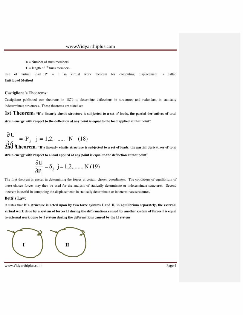
1st Theorem: “If a linearly elastic structure is subjected to a set of loads, the partial derivatives of total
strain energy with respect to the deflection at any point is equal to the load applied at that point”
2nd Theorem: “If a linearly elastic structure is subjected to a set of loads, the partial derivatives of total
strain energy with respect to a load applied at any point is equal to the deflection at that point”
The first theorem is useful in determining the forces at certain chosen coordinates. The conditions of equilibrium of
these chosen forces may then be used for the analysis of statically determinate or indeterminate structures. Second
theorem is useful in computing the displacements in statically determinate or indeterminate structures.
Betti’s Law:
It states that If a structure is acted upon by two force systems I and II, in equilibrium separately, the external
virtual work done by a system of forces II during the deformations caused by another system of forces I is equal
to external work done by I system during the deformations caused by the II system
(18) N ..... 1,2, j P δ
Uj
j
==∂
∂
(19) N .1,2,......j δ P
Uj
j
==∂
∂
I II

www.Vidyarthiplus.com
www.Vidyarthiplus.com Page 5
A body subjected to two system of forces is shown in Fig 7. Wij represents work done by ith system of force on
displacements caused by jth
system at the same point. Betti’s law can be expressed as Wij = Wji, where Wji represents
the work done by jth
system on displacement caused by ith
system at the same point.
Trusses Two Dimensional Structures ThreeDimensionalStructures
Conditions of Equilibrium and Static Indeterminacy
A body is said to be under static equilibrium, when it continues to be under rest after application of loads. During
motion, the equilibrium condition is called dynamic equilibrium. In two dimensional system, a body is in equilibrium
when it satisfies following equation.
ΣFx=0 ; ΣFy=0 ; ΣMo=0 ---1.1
Fig. 7

www.Vidyarthiplus.com
www.Vidyarthiplus.com Page 6
To use the equation 1.1, the force components along x and y axes are considered. In three dimensional system
equilibrium equations of equilibrium are
ΣFx=0 ; ΣFy=0 ; ΣFz=0;
ΣMx=0 ; ΣMy=0 ; ΣMz=0; ----1.2
To use the equations of equilibrium (1.1 or 1.2), a free body diagram of the structure as a whole or of any part of
the structure is drawn. Known forces and unknown reactions with assumed direction is shown on the sketch while
drawing free body diagram. Unknown forces are computed using either equation 1.1 or 1.2
Before analyzing a structure, the analyst must ascertain whether the reactions can be computed using equations
of equilibrium alone. If all unknown reactions can be uniquely determined from the simultaneous solution of the
equations of static equilibrium, the reactions of the structure are referred to as statically determinate. If they cannot be
determined using equations of equilibrium alone then such structures are called statically indeterminate structures. If
the number of unknown reactions are less than the number of equations of equilibrium then the structure is statically
unstable.
The degree of indeterminacy is always defined as the difference between the number of unknown forces and the
number of equilibrium equations available to solve for the unknowns. These extra forces are called redundants.
Indeterminacy with respect external forces and reactions are called externally indeterminate and that with respect to
internal forces are called internally indeterminate.
A general procedure for determining the degree of indeterminacy of two-dimensional structures are given below:
NUK= Number of unknown forces
NEQ= Number of equations available
IND= Degree of indeterminacy
IND= NUK - NEQ
Indeterminacy of Planar Frames
For entire structure to be in equilibrium, each member and each joint must be in equilibrium (Fig. 1.9)
NEQ = 3NM+3NJ
NUK= 6NM+NR
IND= NUK – NEQ = (6NM+NR)-(3NM+3NJ)
IND= 3NM+NR-3NJ ----- 1.3
Three independent reaction components
Free body diagram of Members and Joints

www.Vidyarthiplus.com
www.Vidyarthiplus.com Page 7
Degree of Indeterminacy is reduced due to introduction of internal hinge
NC= Number of additional conditions
NEQ = 3NM+3NJ+NC
NUK= 6NM+NR
IND= NUK-NEQ = 3NM+NR-3NJ-NC ------------1.3a
Indeterminacy of Planar Trusses
Members carry only axial forces
NEQ = 2NJ
NUK= NM+NR
IND= NUK – NEQ
IND= NM+NR-2NJ ----- 1.4
Indeterminacy of 3D FRAMES
A member or a joint has to satisfy 6 equations of equilibrium
NEQ = 6NM + 6NJ-NC
NUK= 12NM+NR
IND= NUK – NEQ
IND= 6NM+NR-6NJ-NC ----- 1.5
Indeterminacy of 3D Trusses
A joint has to satisfy 3 equations of equilibrium
NEQ = 3NJ
NUK= NM+NR
IND= NUK – NEQ
IND= NM+NR-3NJ ----- 1.6
Stable Structure:
Another condition that leads to a singular set of equations arises when the body or structure is improperly restrained
against motion. In some instances, there may be an adequate number of support constraints, but their arrangement
may be such that they cannot resist motion due to applied load. Such situation leads to instability of structure. A
structure may be considered as externally stable and internally stable.

www.Vidyarthiplus.com
www.Vidyarthiplus.com Page 8
Externally Stable:
Supports prevents large displacements
No. of reactions ≥ No. of equations
Internally Stable:
Geometry of the structure does not change appreciably
For a 2D truss NM ≥ 2Nj -3 (NR ≥ 3)
For a 3D truss NM ≥ 3Nj -6 (NR ≥ 3)
Examples:
Determine Degrees of Statical indeterminacy and classify the structures
f)

www.Vidyarthiplus.com
www.Vidyarthiplus.com Page 9
a)
b)
c)
d)
e)
f)
NM=2; NJ=3; NR =4; NC=0
IND=3NM+NR-3NJ-NC
IND=3 x 2 + 4 – 3 x 3 -0 = 1
INDETERMINATE
NM=3; NJ=4; NR =5; NC=2
IND=3NM+NR-3NJ-NC
IND=3 x 3 + 5 – 3 x 4 -2 = 0
DETERMINATE
NM=3; NJ=4; NR =5; NC=2
IND=3NM+NR-3NJ-NC
IND=3 x 3 + 5 – 3 x 4 -2 = 0
DETERMINATE
NM=3; NJ=4; NR =3; NC=0
IND=3NM+NR-3NJ-NC
IND=3 x 3 + 3 – 3 x 4 -0 = 0
DETERMINATE
NM=1; NJ=2; NR =6; NC=2
IND=3NM+NR-3NJ-NC
IND=3 x 1 + 6 – 3 x 2 -2 = 1
INDETERMINATE
NM=1; NJ=2; NR =5; NC=1
IND=3NM+NR-3NJ-NC
IND=3 x 1 + 5 – 3 x 2 -1 = 1
INDETERMINATE

www.Vidyarthiplus.com
www.Vidyarthiplus.com Page 10
NM=1; NJ=2; NR =5; NC=1
IND=3NM+NR-3NJ-NC
IND=3 x 1 + 5 – 3 x 2 -1 = 1
INDETERMINATE
Each support has 6 reactions
NM=8; NJ=8; NR =24; NC=0
IND=6NM+NR-6NJ-NC
IND=6 x 8 + 24 – 6 x 8 -0 = 24
INDETERMINATE
Each support has 3 reactions
NM=18; NJ=15; NR =18; NC=0
IND=6NM+NR-6NJ-NC
IND=6 x 18 + 18 – 6 x 15 = 36
INDETERMINATE
Truss NM=2; NJ=3; NR =4;
IND=NM+NR-2NJ
IND= 2 + 4 – 2 x 3 = 0
DETERMINATE

www.Vidyarthiplus.com
www.Vidyarthiplus.com Page 11
Truss NM=11; NJ=6; NR =4; IND=NM+NR-2NJ IND= 11 + 4– 2 x 6 = 3 INDETERMINATE Degree of freedom or Kinematic Indeterminacy
Members of structure deform due to external loads. The minimum number of parameters required to uniquely
describe the deformed shape of structure is called “Degree of Freedom”. Displacements and rotations at various
points in structure are the parameters considered in describing the deformed shape of a structure. In framed structure
the deformation at joints is first computed and then shape of deformed structure. Deformation at intermediate points
on the structure is expressed in terms of end deformations. At supports the deformations corresponding to a reaction
is zero. For example hinged support of a two dimensional system permits only rotation and translation along x and
y directions are zero. Degree of freedom of a structure is expressed as a number equal to number of free
displacements at all joints. For a two dimensional structure each rigid joint has three displacements as shown in
In case of three dimensional structure each rigid joint has six displacement.
• Expression for degrees of freedom
≥3 1. 2D Frames: NDOF = 3NJ – NR NR
≥6 2. 3D Frames: NDOF = 6NJ – NR NR
≥3 3. 2D Trusses: NDOF= 2NJ – NR NR
≥6 4. 3D Trusses: NDOF = 3NJ – NR NR
Where, NDOF is the number of degrees of freedom
In 2D analysis of frames some times axial deformation is ignored. Then NAC=No. of axial condition is deducted
from NDOF
Examples:
1.2 Determine Degrees of Kinermatic Indeterminacy of the structures given below
Truss NM=14; NJ=9; NR =4;
IND=NM+NR-2NJ
IND= 14+ 4 – 2 x 9 = 0
www.Vidyarthiplus.com
www.Vidyarthiplus.com Page 12
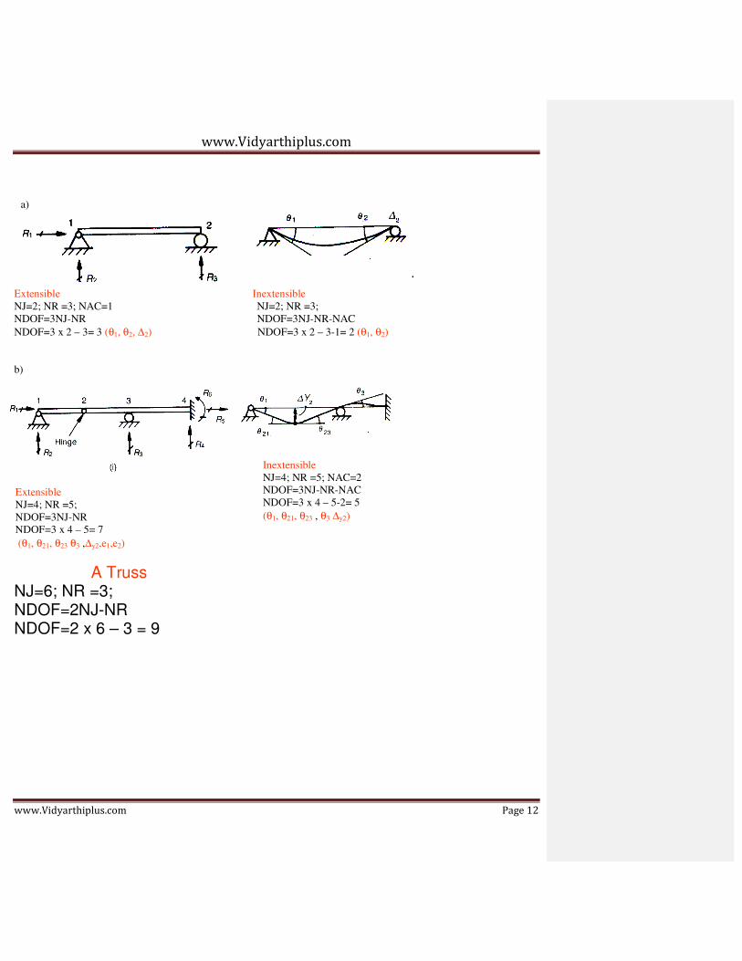
Extensible Inextensible
NJ=2; NR =3; NAC=1 NJ=2; NR =3;
NDOF=3NJ-NR NDOF=3NJ-NR-NAC
NDOF=3 x 2 – 3= 3 (θ1, θ2, ∆2) NDOF=3 x 2 – 3-1= 2 (θ1, θ2)
b)
A Truss NJ=6; NR =3; NDOF=2NJ-NR NDOF=2 x 6 – 3 = 9
a)
Extensible
NJ=4; NR =5;
NDOF=3NJ-NR
NDOF=3 x 4 – 5= 7
(θ1, θ21, θ23 θ3 ,∆y2,e1,e2)
Inextensible
NJ=4; NR =5; NAC=2
NDOF=3NJ-NR-NAC
NDOF=3 x 4 – 5-2= 5
(θ1, θ21, θ23 , θ3 ∆y2)

www.Vidyarthiplus.com
www.Vidyarthiplus.com Page 13
NJ=6; NR =4;
NDOF=2NJ-NR
NDOF=2 x 6 – 4 = 8
Stress-Strain Graph
Virtual Work
Virtual work is defined as the following line integral
where
C is the path or curve traversed by the object, keeping all constraints satisfied;

www.Vidyarthiplus.com
www.Vidyarthiplus.com Page 14
is the force vector;
is the infinitesimal virtual displacement vector.
Virtual work is therefore a special case of mechanical work. For the work to be called virtual, the motion undergone by the
system must be compatible with the system's constraints, hence the use of a virtual displacement.
One of the key ideas of Lagrangian mechanics is that the virtual work done by the constraint forces should be zero. This is a
reasonable assumption, for otherwise a physical system might gain or lose energy simply by being constrained (imagine a
bead on a stationary hoop moving faster and faster for no apparent reason)!
The idea of virtual work also plays a key role in interpreting D'Alembert's principle:
Equilibrium of forces (“staic” treatment)
virtual work produced by inertia force

www.Vidyarthiplus.com
www.Vidyarthiplus.com Page 15
virtual work rpoduced by net applied force.
Note:
Requirements on :
- compatible with the kinematic constraints, but otherwise arbitrary
- instantaneous
- increasingly small
For a single body Bi :
For a system of n bodies B:
“Lagrange form of d’Alembert’s Principle”
This formalism is convenient, as the constraint (non-working) loads disappear. (forces, torques) → where
iis the vector of independent degrees-of-freedom.
Example (i)
The motivation for introducing virtual work can be appreciated by the following simple example from statics of particles.
Suppose a particle is in equilibrium under a set of forces Fxi, Fyi, Fzi i = 1,2,...n:

www.Vidyarthiplus.com
www.Vidyarthiplus.com Page 16
Multiplying the three equations with the respective arbitrary constants δx, δy, δz :
(b)
When the arbitrary constants δx, δy, δz are thought of as virtual displacements of the particle, then the left-hand-sides of (b)
represent the virtual work. The total virtual work is:
(c)
Since the preceding equality is valid for arbitrary virtual displacements, it leads back to the equilibrium equations in (a). The
equation (c) is called the principle of virtual work for a particle. Its use is equivalent to the use of many equilibrium equations.
Applying to a deformable body in equilibrium that undergoes compatible displacements and deformations, we can find the
total virtual work by including both internal and external forces acting on the particles. If the material particles experience
compatible displacements and deformations, the work done by internal stresses cancel out, and the net virtual work done
reduces to the work done by the applied external forces. The total virtual work in the body may also be found by the volume
integral of the product of stresses and virtual strains :
Thus, the principle of virtual work for a deformable body is:

www.Vidyarthiplus.com
www.Vidyarthiplus.com Page 17
This relation is equivalent to the set of equilibrium equations written for the particles in the deformable body. It is valid
irrespective of material behaviour, and hence leads to powerful applications in structural analysis and finite element analysis.
Now consider a block on a surface
Applying formula (c) gives:
leads to
Observe virtual work formalism leads directly to Newton’s equation of motion in the kinematically allowable direction.
Example (ii)
Two bodies connected by a rotary joint.

www.Vidyarthiplus.com
www.Vidyarthiplus.com Page 18
Virtual wotk produced by these constranit loads:
drop out of the expression!
By assuming the contributions to virtual work produced by all forces in and an all system elements, the constraint loads
disappear.
For multi-body system, the derivation of the equatios of motion now becomes much more simple.
Example 1:

www.Vidyarthiplus.com
www.Vidyarthiplus.com Page 19
Note: Internal forces do no work since these forces are always equal and opposite.
Example 2
The physical quantity work is defined as the product of force times a conjugate displacement, i.e., a displacement in the
same direction as the force we are considering. We are familiar with real work, i.e., the product of a real force and a real

www.Vidyarthiplus.com
www.Vidyarthiplus.com Page 20
displacement, i.e., a force and a displacement that both actually occur. The situation is illustrated in Part 1 of the following
figure:
We can extend the concept of real work to a definition of virtual work, which is the product of a real force and a conjugate
displacement, either real or virtual. In Part 2 of the example shown above, we assume that the cantilever column loaded with
force P undergoes a virtual rotation of magnitude θ at its base. We compute the virtual work corresponding to this virtual
displacement by summing the products of real forces times conjugate virtual displacements.
For this calculation, we must introduce unknown sectional forces at those locations where we have cut the structure to create
the virtual displacement. In the example shown above, therefore, we have introduced bending moment at the base, Mb. For
completeness, we would also have to introduce a shear force V and an axial force N at the base of the column, but, as we
shall see, there is no component of virtual displacement conjugate to these forces. They have therefore not been shown in
the example.
We calculate the virtual displacements of the structure corresponding to all known and unknown forces. For a rotation θ at
the base, horizontal translation of the tip of the cantilever is θ · L. We then multiply force times displacement and sum these
products to obtain the following expression for virtual work corresponding to the assumed virtual displacement:
U = P · L · θ – Mb · θ

www.Vidyarthiplus.com
www.Vidyarthiplus.com Page 21
We treat the virtual work done by force Mb as negative since the direction of Mb as drawn is opposite to the direction of the
virtual rotation θ.
The principle of virtual work states that a system of real forces is in equilibrium if and only if the virtual work performed by
these forces is zero for all virtual displacements that are compatible with geometrical boundary conditions.
For the example given in the previous subsection, this implies that the virtual work of the simple cantilever, U, must be zero
for the system to be in equilibrium:
U = P · L · θ – Mb · θ = 0
Since θ is nonzero, it follows that Mb = P · L, which is precisely the familiar expression for bending moment at the base of a
cantilever loaded with force P at its tip.
A more general mathematical statement of the principle of virtual work is as follows:
Let Qi be a set of real loads acting on a given structure
Let Ri be the corresponding real support reactions
Let Mi, Vi, and Ni be the sectional forces (bending moment, shear, and axial force) introduced at the locations where the
structure has been cut to allow it to undergo a virtual displacement.
Let δQi, δRi, δMi, δVi, and δNi be virtual displacements compatible with the geometrical boundary conditions and conjugate to
the forces defined previously.
Then the structure is in equilibrium if and and only if:
Σ(Qi · δQi) + Σ(Ri · δRi) + Σ(Mi · δMi) + Σ(Vi · δVi) + Σ(Ni · δNi) = 0
Williot diagram The Williot diagram is a graphical method to obtain an approximate value for displacement of a structure which
submitted to a certain load. The method consists of, from a graph representation of a structural system, representing the
structure's fixed vertices as a single, fixed starting point and from there sequentially adding the neighbouring vertices'
relative displacements due to strain

www.Vidyarthiplus.com
www.Vidyarthiplus.com Page 22

www.Vidyarthiplus.com
www.Vidyarthiplus.com Page 23
II-UNIT-MOVING LOADS AND INFLUENCE LINES
In engineering, an influence line graphs the variation of a function (such as the shear felt in a structure member) at a
specific point on a beam or truss caused by a unit load placed at any point along the structure.[1][2][3][4][5]
Some of the
common functions studied with influence lines include reactions (the forces that the structure’s supports must apply in
order for the structure to remain static), shear, moment, and deflection. Influence lines are important in the designing
beams and trusses used in bridges, crane rails, conveyor belts, floor girders, and other structures where loads will move
along their span.[5]
The influence lines show where a load will create the maximum effect for any of the functions
studied.
Influence lines are both scalar and additive.[5]
This means that they can be used even when the load that will be applied
is not a unit load or if there are multiple loads applied. To find the effect of any non-unit load on a structure, the ordinate
results obtained by the influence line are multiplied by the magnitude of the actual load to be applied. The entire
influence line can be scaled, or just the maximum and minimum effects experienced along the line. The scaled
maximum and minimum are the critical magnitudes that must be designed for in the beam or truss.
In cases where multiple loads may be in effect, the influence lines for the individual loads may be added together in
order to obtain the total effect felt by the structure at a given point. When adding the influence lines together, it is
necessary to include the appropriate offsets due to the spacing of loads across the structure. For example, if it is known
that load A will be three feet in front of load B, then the effect of A at x feet along the structure must be added to the
effect of B at (x – 3) feet along the structure—not the effect of B at x feet along the structure Many loads are distributed
rather than concentrated. Influence lines can be used with either concentrated or distributed loadings. For a concentrated
(or point) load, a unit point load is moved along the structure. For a distributed load of a given width, a unit-distributed
load of the same width is moved along the structure, noting that as the load nears the ends and moves off the structure
only part of the total load is carried by the structure. The effect of the distributed unit load can also be obtained by
integrating the point load’s influence line over the corresponding length of the structures.

www.Vidyarthiplus.com
www.Vidyarthiplus.com Page 24
When designing a beam or truss, it is necessary to design for the scenarios causing the maximum expected reactions, shears, and moments within the structure members in order to ensure that no member will fail during the life of the
structure. When dealing with dead loads (loads that never move, such as the weight of the structure itself), this is
relatively easy because the loads are easy to predict and plan for. For live loads (any load that will be moved during the
life of the structure, such as furniture and people), it becomes much harder to predict where the loads will be or how
concentrated or distributed they will be throughout the life of the structure.
Influence lines graph the response of a beam or truss as a unit load travels across it. The influence line allows the
designers to discover quickly where to place a live load in order to calculate the maximum resulting response for each of
the following functions: reaction, shear, or moment. The designer can then scale the influence line by the greatest
expected load to calculate the maximum response of each function for which the beam or truss must be designed.
Influence lines can also be used to find the responses of other functions (such as deflection or axial force) to the applied
unit load, but these uses of influence lines is less common.
Influence Lines The major difference between shear and moment diagrams as compared to influence lines is that shear and bending moment diagrams show the variation of the shear and the moment over the entire structure for loads at a fixed position. An influence line for shear or moment shows the variation of the function at one section cause by a moving load. Influence lines for functions of deterministic structures consists of a set of straight lines. The shape of influence lines for truss members are a bit more deceptive.

www.Vidyarthiplus.com
www.Vidyarthiplus.com Page 25
What we have looked at is quantitative influence lines. These have numerical values and can be computed. Qualitative influence lines are based on a principle by Heinrich Müller Breslau, which states: " The deflected shape of a structure represents to some scale the influence line for a function such as reaction, shear or moment, if the function in question is allowed to act through a small distance. " In other words, is that the structure draws its own influence lines from the deflection curves. The shape of the influence lines can be created by deflecting the location in question by a moment, or shear or displacement to get idea of the behavior of the influence line. Realizing that the supports are zero values or poles. Müller's principle for statically determinate structures is useful, but for indeterminated structures it is of great value. You can get an idea of the behavior of the shear and moment at a point in the beam.
Using influence lines to calculate values From the previous examples of a twenty foot beam for the reactions, shear, and moment. We can use the values from the influence lines to calculate the shear and moment at a point.
RAy = Σ (Fi)* Value of the influence line of RAy @ location of the force
V11 = Σ (Fi)* Value of the influence line of V11 @ location of the force
M11 = Σ (Fi)* Value of the influence line of M11 @ location of the force
If we are looking at the forces due to uniform loads over the beam at point. The shear or moment is equal to the area under the influence line times the distributed load.
RAy = Σ (wi)* Area of the influence line of RAy over which w covers
V11 = Σ (wi)* Area of the influence line of V11 over which w covers
M11 = Σ (wi)* Area of the influence line of M11 over which w covers
For moving set of loads the influence lines can be used to calculate the maximum function. This can be done by moving the loads over the influence line find where they will generate the largest value for the particular point.
Panels or floating floor The method can be extend to deal with floor joist and floating floors in which we deal with panels, which are simple beam elements acting on the floor joist. You will need to find the fore as function of the intersection. You are going to find the moment and the shear as you move across the surface of the beam. An example problem is used to show how this can be used to find the shear and moment at a point for a moving load. This technique is similar to that used in truss members.
Methods for constructing influence lines
There are three methods used for constructing the influence line. The first is to tabulate the influence values for multiple
points along the structure, then use those points to create the influence line. The second is to determine the influence-
line equations that apply to the structure, thereby solving for all points along the influence line in terms of x, where x is
the number of feet from the start of the structure to the point where the unit load is applied. The third method is called

www.Vidyarthiplus.com
www.Vidyarthiplus.com Page 26
the Müller-Breslau principle. It creates a qualitative influence line. This nfluence line will still provide the designer with
an accurate idea of where the unit load will produce the largest response of a function at the point being studied, but it
cannot be used directly to calculate what the magnitude that response will be, whereas the influence lines produced by
the first two methods can.
Influence-line equations
It is possible to create equations defining the influence line across the entire span of a structure. This is done by solving
for the reaction, shear, or moment at the point A caused by a unit load placed at x feet along the structure instead of a
specific distance. This method is similar to the tabulated values method, but rather than obtaining a numeric solution,
the outcome is an equation in terms of x.[5]
It is important to understanding where the slope of the influence line changes for this method because the influence-line
equation will change for each linear section of the influence line. Therefore, the complete equation will be a piecewise
linear function which has a separate influence-line equation for each linear section of the influence line.[5]
Müller-Breslau Principle
The Müller-Breslau Principle can be utilized to draw qualitative influence lines, which are directly proportional to the
actual influence line.”[2]
Instead of moving a unit load along a beam, the Müller-Breslau Principle finds the deflected
shape of the beam caused by first releasing the beam at the point being studied, and then applying the function (reaction,
shear, or moment) being studied to that point. The principle states that the influence line of a function will have a scaled
shape that is the same as the deflected shape of the beam when the beam is acted upon by the function.
In order to understand how the beam will deflect under the function, it is necessary to remove the beam’s capacity to
resist the function. Below are explanations of how to find the influence lines of a simply supported, rigid beam
• When determining the reaction caused at a support, the support is replaced with a roller, which cannot
resist a vertical reaction. Then an upward (positive) reaction is applied to the point where the support
was. Since the support has been removed, the beam will rotate upwards, and since the beam is rigid, it
will create a triangle with the point at the second support. If the beam extends beyond the second support
as a cantilever, a similar triangle will be formed below the cantilevers position. This means that the
reaction’s influence line will be a straight, sloping line with a value of zero at the location of the second
support.
• When determining the shear caused at some point B along the beam, the beam must be cut and a roller-
guide (which is able to resist moments but not shear) must be inserted at point B. Then, by applying a
positive shear to that point, it can be seen that the left side will rotate down, but the right side will rotate
up. This creates a discontinuous influence line which reaches zero at the supports and whose slope is
equal on either side of the discontinuity. If point B is at a support, then the deflection between point B
and any other supports will still create a triangle, but if the beam is cantilevered, then the entire
cantilevered side will move up or down creating a rectangle.
• When determining the moment caused by at some point B along the beam, a hinge will be placed at point
B, releasing it to moments but resisting shear. Then when a positive moment is placed at point B, both
sides of the beam will rotate up. This will create a continuous influence line, but the slopes will be equal
and opposite on either side of the hinge at point B. Since the beam is simply supported, its end supports
(pins) cannot resist moment; therefore, it can be observed that the supports will never experience
moments in a static situation regardless of where the load is placed.

www.Vidyarthiplus.com
www.Vidyarthiplus.com Page 27
The Müller-Breslau Principle can only produce qualitative influence lines. This means that engineers can use it to
determine where to place a load to incur the maximum of a function, but the magnitude of that maximum cannot be
calculated from the influence line. Instead, the engineer must use statics to solve for the functions value in that loading
case.
For example, the influence line for the support reaction at A of the structure shown in Figure 1, is found by applying a
unit load at several points (See Figure 2) on the structure and determining what the resulting reaction will be at A. This
can be done by solving the support reaction YA as a function of the position of a downward acting unit load. One such
equation can be found by summing moments at Support B.
Figure 1 - Beam structure for influence line example
Figure 2 - Beam structure showing application of unit load
MB = 0 (Assume counter-clockwise positive moment)
-YA(L)+1(L-x) = 0
YA = (L-x)/L = 1 - (x/L)
The graph of this equation is the influence line for the support reaction at A (See Figure 3). The graph illustrates that if
the unit load was applied at A, the reaction at A would be equal to unity. Similarly, if the unit load was applied at B, the
reaction at A would be equal to 0, and if the unit load was applied at C, the reaction at A would be equal to -e/L.
Figure 3 - Influence line for the support reaction at A
Once an understanding is gained on how these equations and the influence lines they produce are developed, some
general properties of influence lines for statically determinate structures can be stated.
1. For a statically determinate structure the influence line will consist of only straight line segments between
critical ordinate values.
2. The influence line for a shear force at a given location will contain a translational discontinuity at this location.
The summation of the positive and negative shear forces at this location is equal to unity.
3. Except at an internal hinge location, the slope to the shear force influence line will be the same on each side of
the critical section since the bending moment is continuous at the critical section.
4. The influence line for a bending moment will contain a unit rotational discontinuity at the point where the
bending moment is being evaluated.
5. To determine the location for positioning a single concentrated load to produce maximum magnitude for a
particular function (reaction, shear, axial, or bending moment) place the load at the location of the maximum

www.Vidyarthiplus.com
www.Vidyarthiplus.com Page 28
ordinate to the influence line. The value for the particular function will be equal to the magnitude of the
concentrated load, multiplied by the ordinate value of the influence line at that point.
6. To determine the location for positioning a uniform load of constant intensity to produce the maximum
magnitude for a particular function, place the load along those portions of the structure for which the ordinates to
the influence line have the same algebraic sign. The value for the particular function will be equal to the
magnitude of the uniform load, multiplied by the area under the influence diagram between the beginning and
ending points of the uniform load.
There are two methods that can be used to plot an influence line for any function. In the first, the approach described
above, is to write an equation for the function being determined, e.g., the equation for the shear, moment, or axial force
induced at a point due to the application of a unit load at any other location on the structure. The second approach,
which uses the Müller Breslau Principle, can be utilized to draw qualitative influence lines, which are directly
proportional to the actual influence line.
The following examples demonstrate how to determine the influence lines for reactions, shear, and bending moments of
beams and frames using both methods described above.
For example, the influence line for the support reaction at A of the structure shown in Figure 1, is found by applying a
unit load at several points (See Figure 2) on the structure and determining what the resulting reaction will be at A. This
can be done by solving the support reaction YA as a function of the position of a downward acting unit load. One such
equation can be found by summing moments at Support B.
Figure 1 - Beam structure for influence line example
Figure 2 - Beam structure showing application of unit load
MB = 0 (Assume counter-clockwise positive moment)
-YA(L)+1(L-x) = 0
YA = (L-x)/L = 1 - (x/L)
The graph of this equation is the influence line for the support reaction at A (See Figure 3). The graph illustrates that if
the unit load was applied at A, the reaction at A would be equal to unity. Similarly, if the unit load was applied at B, the
reaction at A would be equal to 0, and if the unit load was applied at C, the reaction at A would be equal to -e/L.
Figure 3 - Influence line for the support reaction at A

www.Vidyarthiplus.com
www.Vidyarthiplus.com Page 29
problem statement
Draw the influence lines for the reactions YA, YC, and the shear and bending moment at point B, of the simply supported
beam shown by developing the equations for the respective influence lines.
Figure 1 - Beam structure to analyze
� Reaction YA
The influence line for a reaction at a support is found by independently applying a unit load at several points on the
structure and determining, through statics, what the resulting reaction at the support will be for each case. In this
example, one such equation for the influence line of YA can be found by summing moments around Support C.
Figure 2 - Application of unit load
MC = 0 (Assume counter-clockwise positive moment)
-YA(25)+1(25-x) = 0
YA = (25-x)/25 = 1 - (x/25)
The graph of this equation is the influence line for YA (See Figure 3). This figure illustrates that if the unit load is
applied at A, the reaction at A will be equal to unity. Similarly, if the unit load is applied at B, the reaction at A will be
equal to 1-(15/25)=0.4, and if the unit load is applied at C, the reaction at A will be equal to 0.
Figure 3 - Influence line for YA, the support reaction at A
The fact that YA=1 when the unit load is applied at A and zero when the unit load is applied at C can be used to quickly
generate the influence line diagram. Plotting these two values at A and C, respectively, and connecting them with a
straight line will yield the the influence line for YA. The structure is statically determinate, therefore, the resulting
function is a straight line.
� Reaction at C

www.Vidyarthiplus.com
www.Vidyarthiplus.com Page 30
The equation for the influence line of the support reaction at C is found by developing an equation that relates the
reaction to the position of a downward acting unit load applied at all locations on the structure. This equation is found
by summing the moments around support A.
Figure 4 - Application of unit load
MA = 0 (Assume counter-clockwise positive moment)
YC(25)-1(x) = 0
YC = x/25
The graph of this equation is the influence line for YC. This shows that if the unit load is applied at C, the reaction at C
will be equal to unity. Similarly, if the unit load is applied at B, the reaction at C will be equal to 15/25=0.6. And, if the
unit load is applied at A, the reaction at C will equal to 0.
Figure 5 - Influence line for the reaction at support C
The fact that YC=1 when the unit load is applied at C and zero when the unit load is applied at A can be used to quickly
generate the influence line diagram. Plotting these two values at A and C, respectively, and connecting them with a
straight line will yield the the influence line for YC. Notice, since the structure is statically determinate, the resulting
function is a straight line.
� Shear at B
The influence line for the shear at point B can be found by developing equations for the shear at the section using
statics. This can be accomplished as follows:
a) if the load moves from B to C, the shear diagram will be as shown in Fig. 6 below, this demonstrates that the shear at
B will equal YA as long as the load is located to the right of B, i.e., VB = YA. One can also calculate the shear at B from
the Free Body Diagram (FBD) shown in Fig. 7.
Figure 6 - Shear diagram for load located between B and C

www.Vidyarthiplus.com
www.Vidyarthiplus.com Page 31
Figure 7 - Free body diagram for section at B with a load located between B and C
b) if the load moves from A to B, the shear diagram will be as shown in Fig. 8, below, this demonstrates that the shear at
B will equal -YC as long as the load is located to the left of B, i.e., VB = - YC. One can also calculate the shear at B from
the FBD shown in Fig. 9.
Figure 8 - Shear diagram for load located between A and B
Figure 9 - Free body diagram for section at B with a load located between A and B
The influence line for the Shear at point B is then constructed by drawing the influence line for YA and negative YC.
Then highlight the portion that represents the sides over which the load was moving. In this case, highlight the the part
from B to C on YA and from A to B on -YC. Notice that at point B, the summation of the absolute values of the positive
and negative shear is equal to 1.
Figure 10 - Influence line for shear at point B
� Moment at B
The influence line for the moment at point B can be found by using statics to develop equations for the moment at the
point of interest, due to a unit load acting at any location on the structure. This can be accomplished as follows.
a) if the load is at a location between B and C, the moment at B can be calculated by using the FBD shown in Fig. 7
above, e.g., at B, MB = 15 YA - notice that this relation is valid if and only if the load is moving from B to C.
b) if the load is at a location between A and B, the moment at B can be calculated by using the FBD shown in Fig. 9
above, e.g., at B, MB = 10 YC - notice that this relation is valid if and only if the load is moving from A to B.
The influence line for the Moment at point B is then constructed by magnifying the influence lines for YA and YC by 15
and 10, respectively, as shown below. Having plotted the functions, 15 YA and 10 YC, highlight the portion from B to C
of the function 15 YA and from A to B on the function 10 YC. These are the two portions what correspond to the correct

www.Vidyarthiplus.com
www.Vidyarthiplus.com Page 32
moment relations as explained above. The two functions must intersect above point B. The value of the function at B
then equals (1 x 10 x 15)/25 = 6. This represents the moment at B if the load was positioned at B.
Figure 11 - Influence line for moment at point B
Influence Lines | Index of Examples | CCE Homepage
Influence Lines
Qualitative Influence Lines using the Müller Breslau Principle
� Müller Breslau Principle
The Müller Breslau Principle is another alternative available to qualitatively develop the influence
lines for different functions. The Müller Breslau Principle states that the ordinate value of an influence
line for any function on any structure is proportional to the ordinates of the deflected shape that is
obtained by removing the restraint corresponding to the function from the structure and introducing a
force that causes a unit displacement in the positive direction.
Figure 1 - Beam structure to analyze
For example, to obtain the influence line for the support reaction at A for the beam shown in Figure 1,
above, remove the support corresponding to the reaction and apply a force in the positive direction that
will cause a unit displacement in the direction of YA. The resulting deflected shape will be proportional
to the true influence line for this reaction. i.e., for the support reaction at A. The deflected shape due to
a unit displacement at A is shown below. Notice that the deflected shape is linear, i.e., the beam rotates
as a rigid body without any curvature. This is true only for statically determinate systems.
Figure 2 - Support removed, unit load applied, and resulting influence line for support reaction at A
Similarly, to construct the influence line for the support reaction YB, remove the support at B and apply
a vertical force that induces a unit displacement at B. The resulting deflected shape is the qualitative
influence line for the support reaction YB.

www.Vidyarthiplus.com
www.Vidyarthiplus.com Page 33
Figure 3 - Support removed, unit load applied, and resulting influence line for support reaction at B
Once again, notice that the influence line is linear, since the structure is statically determinate.
This principle will be now be extended to develop the influence lines for other functions.
� Shear at s
To determine the qualitative influence line for the shear at s, remove the shear resistance of the beam at
this section by inserting a roller guide, i.e., a support that does not resist shear, but maintains axial
force and bending moment resistance.
Figure 4 - Structure with shear capacity removed at s
Removing the shear resistance will then allow the ends on each side of the section to move
perpendicular to the beam axis of the structure at this section. Next, apply a shear force, i.e., Vs-R and
Vs-L that will result in the relative vertical displacement between the two ends to equal unity. The
magnitude of these forces are proportional to the location of the section and the span of the beam. In
this case,
Vs-L = 1/16 x 10 = 10/16 = 5/8
Vs-R = 1/16 x 6 = 6/16 = 3/8
The final influence line for Vs is shown below.
Figure 5 - Influence line for shear at s
� Shear just to the left side of B
The shear just to the left side of support B can be constructed using the ideas explained above. Simply
imagine that section s in the previous example is moved just to the left of B. By doing this, the
magnitude of the positive shear decreases until it reaches zero, while the negative shear increases to 1.

www.Vidyarthiplus.com
www.Vidyarthiplus.com Page 34
Figure 6 - Influence line for shear just to the left of B
� Shear just to the right side of B
To plot the influence line for the shear just to the right side of support B, Vb-R, release the shear just to
the right of the support by introducing the type of roller shown in Fig. 7, below. The resulting deflected
shape represents the influence line for Vb-R. Notice that no deflection occurs between A and B, since
neither of those supports were removed and hence the deflections at A and B must remain zero. The
deflected shape between B and C is a straight line that represents the motion of a rigid body.
Figure 7 - Structure with shear capacity removed at just to the right of B and the resulting influence
line
� Moment at s
To obtain a qualitative influence line for the bending moment at a section, remove the moment restraint
at the section, but maintain axial and shear force resistance. The moment resistance is eliminated by
inserting a hinge in the structure at the section location. Apply equal and opposite moments
respectively on the right and left sides of the hinge that will introduce a unit relative rotation between
the two tangents of the deflected shape at the hinge. The corresponding elastic curve for the beam,
under these conditions, is the influence line for the bending moment at the section. The resulting
influence line is shown below.
Figure 8 - Structure with moment capacity removed at s and the resulting influence line
The values of the moments shown in Figure 8, above, are calculated as follows:
a. when the unit load is applied at s, the moment at s is YA x 10 = 3/8 x 10 = 3.75
(see the influence line for YA, Figure 2, above, for the value of YA with a unit load applied at s)
b. when the unit load is applied at C, the moment at s is YA x 10 = -3/8 x 10 = -3.75
(again, see the influence line for YA for the value of YA with a unit load applied at C)
Following the general properties of influence lines, given in the Introduction, these two values are
plotted on the beam at the locations where the load is applied and the resulting influence line is
constructed.

www.Vidyarthiplus.com
www.Vidyarthiplus.com Page 35
� Moment at B
The qualitative influence line for the bending moment at B is obtained by introducing a hinge at
support B and applying a moment that introduces a unit relative rotation. Notice that no deflection
occurs between supports A and B since neither of the supports were removed. Therefore, the only
portion that will rotate is part BC as shown in Fig. 9, below.
Figure 9 - Structure with moment capacity removed at B and the resulting influence line
� Shear and moment envelopes due to uniform dead and live loads
The shear and moment envelopes are graphs which show the variation in the minimum and maximum
values for the function along the structure due to the application of all possible loading conditions. The
diagrams are obtained by superimposing the individual diagrams for the function based on each
loading condition. The resulting diagram that shows the upper and lower bounds for the function along
the structure due to the loading conditions is called the envelope.
The loading conditions, also referred to as load cases, are determined by examining the influence lines
and interpreting where loads must be placed to result in the maximum values. To calculate the
maximum positive and negative values of a function, the dead load must be applied over the entire
beam, while the live load is placed over either the respective positive or negative portions of the
influence line. The value for the function will be equal to the magnitude of the uniform load, multiplied
by the area under the influence line diagram between the beginning and ending points of the uniform
load.
For example, to develop the shear and moment envelopes for the beam shown in Figure 1, first sketch
the influence lines for the shear and moment at various locations. The influence lines for Va-R, Vb-L, Vb-
R, Mb, Vs, and Ms are shown in Fig. 10.

www.Vidyarthiplus.com
www.Vidyarthiplus.com Page 36
Figure 10 - Influence lines
These influence lines are used to determine where to place the uniform live load to yield the maximum
positive and negative values for the different functions. For example;
Figure 11 - Support removed, unit load applied, and resulting influence line for support reaction at A
The maximum value for the positive reaction at A, assuming no partial loading, will occur when the
uniform load is applied on the beam from A to B (load case 1)
Figure 12 - Load case 1
The maximum negative value for the reaction at A will occur if a uniform load is placed on the
beam from B to C (load case 2)
Figure 13 - Load case 2
Load case 1 is also used for:
• maximum positive value of the shear at the right of support A
• maximum positive moment Ms

www.Vidyarthiplus.com
www.Vidyarthiplus.com Page 37
Load case 2 is also used for:
• maximum positive value of the shear at the right of support B
• maximum negative moments at support B and Ms
Load case 3 is required for:
• maximum positive reaction at B
• maximum negative shear on the left side of B
Figure 14 - Load case 3
Load case 4 is required for the maximum positive shear force at section s
Figure 15 - Load case 4
Load case 5 is required for the maximum negative shear force at section s
Figure 16 - Load case 5
To develop the shear and moment envelopes, construct the shear and moment diagrams for each load
case. The envelope is the area that is enclosed by superimposing all of these diagrams. The maximum
positive and negative values can then be determined by looking at the maximum and minimum values
of the envelope at each point.
Individual shear diagrams for each load case;

www.Vidyarthiplus.com
www.Vidyarthiplus.com Page 38
Figure 17 - Individual shear diagrams
Superimpose all of these diagrams together to determine the final shear envelope.
Figure 18 - Resulting superimposed shear envelope
Individual moment diagrams for each load case;

www.Vidyarthiplus.com
www.Vidyarthiplus.com Page 39
Figure 19 - Individual moment diagrams
Superimpose all of these diagrams together to determine the final moment envelope.
Figure 20 - Resulting superimposed moment envelope
Influence Lines | Index of Examples | CCE Homepage
Influence Lines
Qualitative Influence Lines for a Statically Determinate Continuous Beam
problem statement
Draw the qualitative influence lines for the vertical reactions at the supports, the shear and moments at sections s1 and
s2, and the shear at the left and right of support B of the continuous beam shown.

www.Vidyarthiplus.com
www.Vidyarthiplus.com Page 40
Figure 1 - Beam structure to analyze
� Reactions at A, B, and C
Qualitative influence lines for the support reactions at A, B, and C are found by using the Müller Breslau Principle for
reactions, i.e., apply a force which will introduce a unit displacement in the structure at each support. The resulting
deflected shape will be proportional to the influence line for the support reactions.
The resulting influence lines for the support reactions at A, B, and C are shown in Figure 2, below.
Figure 2 - Influence lines for the reactions at A, B, and C
Note: Beam BC does not experience internal forces or reactions when the load moves from A to h. In other words,
influence lines for beam hC will be zero as long as the load is located between A and h. This can also be explained by
the fact that portion hC of the beam is supported by beam ABh as shown in Figure 3, below.
Figure 3 - Beam hC supported by beam ABh
Therefore, the force Yh required to maintain equilibrium in portion hC when the load from h to C is provided by portion
ABh. This force, Yh, is equal to zero when the load moves between A an h, and hence, no shear or moment will be
induced in portion hC.

www.Vidyarthiplus.com
www.Vidyarthiplus.com Page 41
� Shear and moment at section S1 and S2
To determine the shear at s1, remove the shear resistance of the beam at the section by inserting a support that does not
resist shear, but maintains axial force and bending moment resistance (see the inserted support in Figure 4). Removing
the shear resistance will allow the ends on each side of the section to move perpendicular to the beam axis of the
structure at this section. Next, apply shear forces on each side of the section to induce a relative displacement between
the two ends that will equal unity. Since the section is cut at the midspan, the magnitude of each force is equal to 1/2.
Figure 4 - Structure with shear capacity removed at s1 and resulting influence line
For the moment at s1, remove the moment restraint at the section, but maintain axial and shear force resistance. The
moment resistance is eliminated by inserting a hinge in the structure at the section location. Apply equal and opposite
moments on the right and left sides of the hinge that will introduce a unit relative rotation between the two tangents of
the deflected shape at the hinge. The corresponding elastic curve for the beam, under these conditions, is the influence
line for the bending moment at the section.
Figure 5 - Structure with moment capacity removed at s1 and resulting influence line
The value of the moment shown in Figure 5, above, is equal to the value of Ra when a unit load is applied at s1,
multiplied by the distance from A to s1. Ms1 = 1/2 x 4 = 2.
The influence lines for the shear and moment at section s2 can be constructed following a similar procedure. Notice that
when the load is located between A and h, the magnitudes of the influence lines are zero for the shear and moment at s1.
The was explained previously in the discussion of the influence line for the support reaction at C (see Figures 2 and 3).
Figure 6 - Structure with shear capacity removed at s2 and resulting influence line

www.Vidyarthiplus.com
www.Vidyarthiplus.com Page 42
Figure 7 - Structure with moment capacity removed at s2 and resulting influence line
� Shear at the left and right of B
Since the shear at B occurs on both sides of a support, it is necessary to independently determine the shear for each side.
To plot the influence line for Vb-L, follow the instructions outlined above for plotting the influence line for the shear at
s1. To construct the shear just to the left of support B, imagine that the section s1 has been moved to the left of B. In this
case, the positive ordinates of the influence line between A and B will decrease to zero while the negative ordinates will
increase to 1 (see Figure 8).
Figure 8 - Structure with shear capacity removed at the left of B and the resulting influence line
The influence line for the shear forces just to the right of support B, Vb-R, is represented by the resulting deflected shape
of the beam induced by shear forces acting just to the right of support B. Notice that the portion of the beam from B to h
moves as a rigid body (see explanation in the Simple Beam with a Cantilever example) while the influence line varies
linearly from h to C. This is due to the fact that the deflection at C is zero and the assumption that the deflection of a
statically determinate system is linear.
Figure 9 - Structure with shear capacity removed at the right of B and the resulting influence line
Influence Lines | Index of Examples | CCE Homepage

www.Vidyarthiplus.com
www.Vidyarthiplus.com Page 43
Influence Lines
Calculation of Maximum and Minimum Shear Force and Moments on a Statically Determinate Continuous Beam
problem statement
Determine the resulting forces for RA, RB, RC, Ms1, Vs1, Ms1, Vs2, VBL, and VBR under a uniform live load of 2 k/ft and a
uniform dead load of 3 k/ft for the beam below.
note: influence lines for this beam are developed in the Statically Determinate Continuous Beam example.
Figure 1 - Beam structure to analyze
� Influence lines
From the Continuous Beam with a Hinge example, the required influence lines for the structure are:

www.Vidyarthiplus.com
www.Vidyarthiplus.com Page 44
� Calculate forces
In order to calculate the forces due to uniform dead and live loads on a structure, a relationship between the influence
line and the uniform load is required. Referring to Figure 2, each segment dx, of a uniform load w, creates an equivalent
concentrated load, dF = w dx, acting a distance x from an origin.
From the general properties for influence lines, given in the introduction, it is known that the resulting value of the
function for a force acting at a point is equivalent to the magnitude of the force, dF, multiplied by the ordinate value, y,
of the influence line at the point of application.
Figure 2 - Equivalent concentrated load
In order to determine the effect of the uniform load, the effect of all series loads, dF, must be determined for the beam.
This is accomplished by integrating y dF over the length of the beam, i.e., w y dx = w y dx. The integration of y
dx equal to the area under the influence line. Thus, the value of the function caused by a uniform load is equal to the
magnitude of the uniform load multiplied by the area under the influence line diagram.
In order to find the resulting minimum and maximum values for the reactions, shears, and moments required, create a
table which contains the resulting positive and negative values for the areas enclosed by the influence lines for each
function. The effect of the dead load is determined by multiplying the net area under the influence line by the dead load.
For the live load, multiply the respective positive and negative areas by the live load, yields to the positive and negative
forces, respectively. The resulting maximum and minimum forces for dead load plus the effects of positive and negative
live loads are then found by adding the respective values.
The resulting forces due to a uniformly distributed dead load = 3 k/ft and a live load = 2 k/ft applied to the beam above,
are as follows:
Force
I
Positive area
under the influence line
II
Negative area
under the influence line
III
Net area
IV
Force
due to DL
V
Positive
force due to LL
VI
Negative
force due to LL
VII
Maximum
force (DL+LL)
VIII
Minimum
force (DL-LL)
IX
RA 4 -1 3 9 8 -2 17 7
RB 10 - 10 30 20 - 50 30
RC 3 - 3 9 6 - 15 9
www.Vidyarthiplus.com
www.Vidyarthiplus.com Page 45
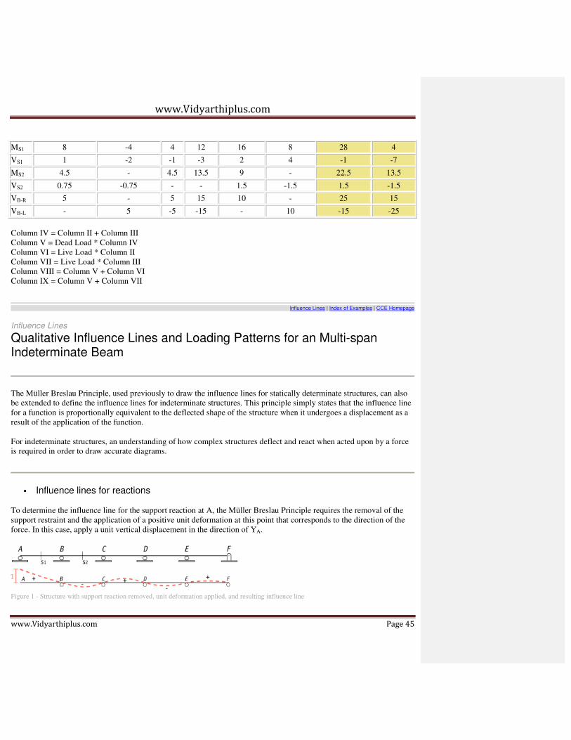
MS1 8 -4 4 12 16 8 28 4
VS1 1 -2 -1 -3 2 4 -1 -7
MS2 4.5 - 4.5 13.5 9 - 22.5 13.5
VS2 0.75 -0.75 - - 1.5 -1.5 1.5 -1.5
VB-R 5 - 5 15 10 - 25 15
VB-L - 5 -5 -15 - 10 -15 -25
Column IV = Column II + Column III
Column V = Dead Load * Column IV
Column VI = Live Load * Column II
Column VII = Live Load * Column III
Column VIII = Column V + Column VI
Column IX = Column V + Column VII
Influence Lines | Index of Examples | CCE Homepage
Influence Lines
Qualitative Influence Lines and Loading Patterns for an Multi-span Indeterminate Beam
The Müller Breslau Principle, used previously to draw the influence lines for statically determinate structures, can also
be extended to define the influence lines for indeterminate structures. This principle simply states that the influence line
for a function is proportionally equivalent to the deflected shape of the structure when it undergoes a displacement as a
result of the application of the function.
For indeterminate structures, an understanding of how complex structures deflect and react when acted upon by a force
is required in order to draw accurate diagrams.
� Influence lines for reactions
To determine the influence line for the support reaction at A, the Müller Breslau Principle requires the removal of the
support restraint and the application of a positive unit deformation at this point that corresponds to the direction of the
force. In this case, apply a unit vertical displacement in the direction of YA.
Figure 1 - Structure with support reaction removed, unit deformation applied, and resulting influence line

www.Vidyarthiplus.com
www.Vidyarthiplus.com Page 46
The resulting deflected shape, due to the application of the unit deformation, is then proportionally equivalent to the
influence line for the support reaction at A. Notice that in statically indeterminate structures, the deflected shape is not a
straight line, but rather a curve. The ordinates of the deflected shape decrease as the distance increases from the point of
application of the unit deformation.
Similarly, for the other support reactions, remove the support restraint and apply a unit deformation in the direction of
the removed restraint. For example, the influence line for the support reaction at C is obtained by removing the reaction
at C and applying a unit displacement in the vertical direction at C. The resulting deflected shape is a qualitative
representation of the influence line at RC (see Figure 2).
Figure 2 - Structure with support reaction removed, unit deformation applied, and resulting influence line
Influence lines for the remaining support reactions are found in a similar manner.
� Influence lines for shears
For shear at a section, using the Müller Breslau Principle, the shear resistance at the point of interest is removed by
introducing the type of support shown in Figure 3, below. Shear forces are applied on each side of the section in order to
produce a relative displacement between the two sides which is equal to unity. The deflected shape of the beam under
these conditions will qualitatively represent the influence line for the shear at the section. Notice that unlike the
statically determinate structure, the magnitude of the shear force on the right and left can not easily be determined.
Figure 3 - Structure with shear carrying capacity removed at section S1, deformations applied, and resulting influence line
� Influence lines for moments
For the moment at a section, using the Müller Breslau Principle, the moment resistance at the point of interest is
removed by introducing a hinge at the section as shown in Figure 4, below. Then a positive moment that introduces a
relative unit rotation is applied at the section. The deflected shape of the beam under these conditions will qualitatively
represent the influence line for the moment at the section.
Figure 4 - Structure with moment capacity removed at section S1, unit rotation applied, and resulting influence line

www.Vidyarthiplus.com
www.Vidyarthiplus.com Page 47
For the moment at a support, the moment resistance is again removed by inserting a hinge at the support. This hinge
only prevents the transfer of moments, so the vertical translation remains fixed due to the support. By applying negative
moments that induces a relative rotation of unity at this section, a deflected shape is generated. Again, this deflected
shape qualitatively represents the influence line for the moment at a support.
Figure 5 - Structure with moment capacity removed at support B, unit rotation applied, and resulting influence line
� Loading cases for moment and shear envelopes
Using the influence lines found above, illustrate the loading cases needed to calculate the maximum positive and
negative RA, RC, MB, VS1, and MS1.
The load cases are generated for the maximum positive and negative values by placing a distributed load on the spans
where the algebraic signs of the influence line are the same. i.e., to get a maximum positive value for a function, place a
distributed load where the influence line for the function is positive.
Figure 6 - Multi-span structure
Load case for maximum positive reaction at support A
Figure 7 - Maximum positive reaction at support A
Load case for maximum negative reaction at support A
Figure 8 - Maximum negative reaction at support A
Load case for maximum positive reaction at support C
Figure 9 - Maximum positive reaction at support C
Load case for maximum negative reaction at support C
Figure 10 - Maximum negative reaction at support C

www.Vidyarthiplus.com
www.Vidyarthiplus.com Page 48
Load case for maximum positive moment at support B
Figure 11 - Maximum positive moment at support B
Load case for maximum negative moment at support B
Figure 12 - Maximum negative moment at support B
Load case for maximum positive shear at s
Figure 13 - Maximum positive shear at s
Load case for maximum negative shear at s
Figure 14 - Maximum negative shear at s
Load case for maximum positive moment at s
Figure 16 - Maximum positive moment at s
Load case for maximum negative moment at s
Figure 17 - Maximum negative moment at s
Influence Lines | Index of Examples | CCE Homepage
Influence Lines
Qualitative Influence Lines and Loading Patterns for an Indeterminate Frame
problem statement
Using the Müller Breslau Principle, draw the influence lines for the moment and shear at the midspan of beam AB, and
the moment at B in member BC. Draw the loading cases to give the maximum positive moment at the midpsan of beam
AB, the maximum and minimum shear at the midspan of beam AB, and the maximum negative moment at B in member
BC in the indeterminate frame below.

www.Vidyarthiplus.com
www.Vidyarthiplus.com Page 49
Figure 1 - Frame structure to analyze
� Influence lines
Influence line for moment at midspan of AB, and the loading case for maximum positive moment at this location.
The influence line for beam ABCD can be constructed by following the procedure outlined in the Multi-span
Indeterminate Beam example. To construct the rest of the influence line, make use of the fact that the angles between a
column and a beam after deformation must be equal to that before deformation. In this example, these angles are 90°.
Therefore, once the deflected shape of beam ABCD is determined, the deflected shape for the columns can be
constructed by keeping the angles between the tangent of the deflect shape of the beam and the column equal to 90° (see
Figure 2).
To get the maximum positive result for the moment, apply a distributed load at all locations where the value of the
influence line is positive (see Figure 3).
Figure 2 - Influence lines for moment at midspan of AB
Figure 3 - Load case for maximum positive moment at midspan of AB
Influence line for shear at the midspan of member AB, and the load case for maximum positive shear at this location.

www.Vidyarthiplus.com
www.Vidyarthiplus.com Page 50
Figure 4 - Influence lines for shear at midspan of AB
Figure 5 - Load case for maximum positive shear at midspan of AB Figure 6 - Load case for maximum negative shear at midspan of AB
Influence line for moment at B in member BC, and the load case for maximum negative moment at this location.
Figure 7 - Influence lines for moment at B Figure 8 - Load case for maximum positive moment at B

www.Vidyarthiplus.com
www.Vidyarthiplus.com Page 51
III-UNIT ARCHES
THREE HINGED ARCHES
An arch is a curved beam in which horizontal movement at the support is wholly or partially prevented. Hence
there will be horizontal thrust induced at the supports. The shape of an arch doesn’t change with loading and therefore
some bending may occur.
Types of Arches On the basis of material used arches may be classified into and steel arches, reinforced concrete arches, masonry
arches etc.,
On the basis of structural behavior arches are classified as :
Three hinged arches:- Hinged at the supports and the crown.
Two hinged arches:- Hinged only at the support
Hinges at the
support
Rib of the arch Rise
Span
Hinged at the
support
Hinged at the
crown
Springing
Rise
Span

www.Vidyarthiplus.com
www.Vidyarthiplus.com Page 52
The supports are fixed
A 3-hinged arch is a statically determinate structure. A 2-hinged arch is an indeterminate structure of degree of
indeterminancy equal to 1. A fixed arch is a statically indeterminate structure. The degree of indeterminancy is 3.
Depending upon the type of space between the loaded area and the rib arches can be classified as open arch or closed
arch (solid arch).
Analysis of 3-hinged arches It is the process of determining external reactions at the support and internal quantities such as normal thrust,
shear and bending moment at any section in the arch.
Procedure to find reactions at the supports Step 1. Sketch the arch with the loads and reactions at the support.
Apply equilibrium conditions namely 0,Fx =∑ 0Fy =∑ 0Mand =∑
Apply the condition that BM about the hinge at the crown is zero (Moment of all the forces either to the left or to the
right of the crown).
Solve for unknown quantities.
A 3-hinged arch has a span of 30m and a rise of 10m. The arch carries UDL of 0.6 kN/m on the left half of the span. It
also carries 2 concentrated loads of 1.6 kN and 1 kN at 5 m and 10 m from the ‘rt’ end. Determine the reactions at the
support. (sketch not given).
∑ = 0Fx
0HHBA
=−
B HB = 4.275
0.6 kN/m C
5 m 5 m
h = 10m
L = 30m VA = 7.35 VB = 4.25
HB = 4.275 A
1 kN 1.6 kN
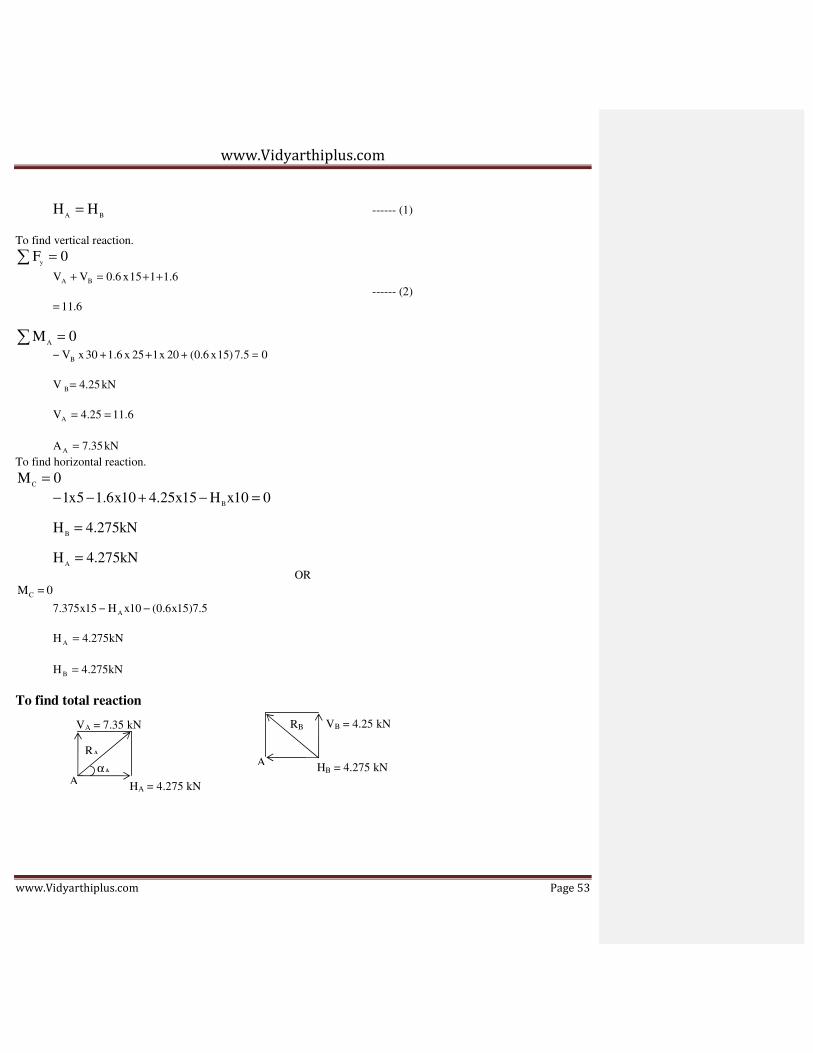
www.Vidyarthiplus.com
www.Vidyarthiplus.com Page 53
BA
HH = ------ (1)
To find vertical reaction.
∑ = 0Fy
6.11
6.1115x6.0VV BA
=
++=+ ------ (2)
∑ = 0MA
kN35.7A
6.1125.4V
kN25.4V
05.7)15x6.0(20x125x6.130xV
A
A
B
B
=
==
=
=+++−
To find horizontal reaction.
0MC
=
kN275.4H
kN275.4H
010xH15x25.410x6.15x1
A
B
B
=
=
=−+−−
OR
0MC =
kN275.4H
kN275.4H
5.7)15x6.0(10xH15x375.7
B
A
A
=
=
−−
To find total reaction
RA
αA
A HA = 4.275 kN
VA = 7.35 kN RB
A HB = 4.275 kN
VB = 4.25 kN

www.Vidyarthiplus.com
www.Vidyarthiplus.com Page 54
83.44H
Vtan
kN02.6VHR
82.59H
Vtan
kN5.8
35.7275.4
VHR
B
B1
B
2
B
2
BB
0
A
A1
A
22
2
A
2
AA
=
=α
=+=
=
=α
=
+
==
−
−
A 3-hinged parabolic arch of span 50m and rise 15m carries a load of 10kN at quarter span as shown in figure.
Calculate total reaction at the hinges.
∑ = 0Fx
BA
HH =
To find vertical reaction.
∑ = 0Fy
10VV BA =+ ------ (1)
∑ = 0MA
kN5.7VkN5.2V
05.12x1050xV
AB
B
==
=+−
To find Horizontal reaction
B HB
10 kN C
15 m
50 m VA VB
HA A
12.5 m

www.Vidyarthiplus.com
www.Vidyarthiplus.com Page 55
0MC =
015H25VBB
=×−×
To find total reaction.
94.30H
Vtan
kN861.4R
VHR
92.60H
Vtan
kN581.8R
5.717.4R
HkN17.4H
0
B
B1
B
B
2
B
2
AB
0
A
A1
A
A
22
A
AB
=
=α
=
+=
=
=α
=
+=
==
−
−
RA
αA
A HA = 4.17
VA = 7.5
RB
HB = 4.17
VB = 4.25

www.Vidyarthiplus.com
www.Vidyarthiplus.com Page 56
Problem: Determine the reaction components at supports A and B for 3-hinged arch shown in fig.
To find Horizontal reaction
∑ = 0Fx
0HHBA
=−
BA
HH = ------ (1)
To find vertical reaction.
∑ = 0Fy
280VV
10x10180VV
BA
BA
=+
+=+ ------ (2)
∑ = 0MA
33.1558V10H
3740V24H4.2
05x10x1018x1804.2xH24xV
BB
BB
BB
−=−
−=−
=+++−
------ (3)
0M C =
B HB
10 kN/m C
2.5 m
10 m
VA
VB
HA A
2 .4 m
180 kN
8 m 6 m

www.Vidyarthiplus.com
www.Vidyarthiplus.com Page 57
87.293V857.2H
144014V9.4xH
09.4xH14xV8x180
BB
BB
BB
+=+−
−=−
=−−−
------ (4)
Adding 2 and 3
AB
B
A
B
BB
HkN67.211H
33.1558177x10H
kN103V
kN177V
87.29333.1558V857.2V10
==
−=−
=
=
+−=+−
Problem: A symmetrical 3-hinged parabolic arch has a span of 20m. It carries UDL of intensity 10 kNm over the entire
span and 2 point loads of 40 kN each at 2m and 5m from left support. Compute the reactions. Also find BM, radial
shear and normal thrust at a section 4m from left end take central rise as 4m.
∑ =0Fx
BA
BA
HH
0HH
=
=− ------ (1)
∑ = 0Fy
280VV
020x104040VV
BA
BA
=+
=−−−+ ------ (2)
C
4 m
20 m
40 kN
M
2 m 3m
10 kN/m 40 kN

www.Vidyarthiplus.com
www.Vidyarthiplus.com Page 58
∑ =0MA
kN166V
kN114V
020xV10)20x10(5x402x40
A
B
B
=
=
=−+++
0M c =
kN160H
kN160H
010x1144xH5)10x10(
A
B
B
=
=
=+−−
BM at M
= - 160 x 2.56
+ 166 x 4 – 40 x 2
- (10 x 4)2
= + 94.4 kNm
( )xLL
hx4y
2−=
( )42020
4x4x42
−=
m56.2y =
tan ( )x2LL
h42
−=φ
= ( )4x22020
4x42
−
VERTICAL
NORMAL
HORIZONT
AL
64.35
160 kN
φ = 25.64 M
REDIAL
10 kN/m
160 kN
4 m
y = 2.56
86 kN
40 kN
2 m
166 kN

www.Vidyarthiplus.com
www.Vidyarthiplus.com Page 59
64.250=φ
Normal thrust = N = + 160 Cos 25.64
+ 86 Cos 64.36
= 181.46 kN
S = 160 Sin 25.64
- 86 x Sin 64.36
S = - 8.29 kN
IV UNIT SLOPE DEFLECTION METHOD
The slope deflection method is a structural analysis method for beams and frames introduced in 1915 by George A.
Maney.[1]
The slope deflection method was widely used for more than a decade until the moment distribution method
was developed.
Introduction
By forming slope deflection equations and applying joint and shear equilibrium conditions, the rotation angles (or the
slope angles) are calculated. Substutituting them back into the slope deflection equations, member end moments are
readily determined.
Slope deflection equations
The slope deflection equations express the member end moments in terms of rotations angles. The slope deflection
equations of member ab of flexural rigidity EIab and length Lab are:
where θa, θb are the slope angles of ends a and b respectively, ∆ is the relative lateral displacement of ends a and b. The
absence of cross-sectional area of the member in these equations implies that the slope deflection method neglects the
effect of shear and axial deformations.
The slope deflection equations can also be written using the stiffness factor and the chord
rotation :

www.Vidyarthiplus.com
www.Vidyarthiplus.com Page 60
Derivation of slope deflection equations
When a simple beam of length Lab and flexural rigidity E Iab is loaded at each end with clockwise moments Mab and Mba,
member end rotations occur in the same direction. These rotation angles can be calculated using the unit dummy force
method or the moment-area theorem.
Rearranging these equations, the slope deflection equations are derived.
Equilibrium conditions
Joint equilibrium
Joint equilibrium conditions imply that each joint with a degree of freedom should have no unbalanced moments i.e. be
in equilibrium. Therefore,
Here, Mmember are the member end moments, Mf are the fixed end moments, and Mjoint are the external moments directly
applied at the joint.
Shear equilibrium
When there are chord rotations in a frame, additional equilibrium conditions, namely the shear equilibrium conditions
need to be taken into account.
DISPLACEMENT METHOD OF ANALYSIS:
SLOPE DEFLECTION EQUATIONS
� General Case
� Stiffness Coefficients

www.Vidyarthiplus.com
www.Vidyarthiplus.com Page 61
� Stiffness Coefficients Derivation
� Fixed-End Moments
� Pin-Supported End Span
� Typical Problems
� Analysis of Beams
� Analysis of Frames: No Sidesway
� Analysis of Frames: Sidesway
1

www.Vidyarthiplus.com
www.Vidyarthiplus.com Page 62
Slope – Deflection Equations
i P w
j k
Cj
settlement = ∆j
i P w
j
Mij Mji
θi
ψ θj

www.Vidyarthiplus.com
www.Vidyarthiplus.com Page 63
2

www.Vidyarthiplus.com
www.Vidyarthiplus.com Page 64
Degrees of Freedom
M θΑ
A B 1 DOF: θΑ
L
P θΑ
A B
C 2 DOF: θΑ , θΒ
θΒ

www.Vidyarthiplus.com
www.Vidyarthiplus.com Page 65
3

www.Vidyarthiplus.com
www.Vidyarthiplus.com Page 66
Stiffness
kAA 1 kBA
A B
L
k AA
kBA
= 4EI
L
= 2EI
L

www.Vidyarthiplus.com
www.Vidyarthiplus.com Page 67
4

www.Vidyarthiplus.com
www.Vidyarthiplus.com Page 68
kAB kBB
A B
L
kBB
k AB
= 4EI
L
= 2EI
L

www.Vidyarthiplus.com
www.Vidyarthiplus.com Page 69
5

www.Vidyarthiplus.com
www.Vidyarthiplus.com Page 70
Fixed-End Forces
Fixed-End Moments: Loads
P
PL L/2 L/2 PL
8 8
L
P
2
w
wL2
12
wL L
2
P
2
wL2
12
wL
2

www.Vidyarthiplus.com
www.Vidyarthiplus.com Page 71
6

www.Vidyarthiplus.com
www.Vidyarthiplus.com Page 72
General Case i
P w
j k
Cj
settlement = ∆j
i P w
j
Mij Mji
θi
ψ θj

www.Vidyarthiplus.com
www.Vidyarthiplus.com Page 73
7

www.Vidyarthiplus.com
www.Vidyarthiplus.com Page 74
(M (M ) ij
Mij
i P w j
θi
L
ψ
Mji
θj
settlement = ∆j
4EI θ
2EI θ
2EI θ
4EI θ
+
L i
L j
= Mij
Mji = i + j
L L θj
θi
+ (MF ) F
ij ∆ (M
+
ji)∆
settlement = ∆j
F )Load
P w
F ji Load

www.Vidyarthiplus.com
www.Vidyarthiplus.com Page 75
F F F
M ij = (
4EI
L
)θi + (
2EI
L
)θ j
+ (M
ij )∆
+ (M
ij ) Load
, M ji
= ( 2EI
L
)θ i + (
4EI
L
)θ j
+ (M
ji )∆
+ (M F
ji ) Load 8

www.Vidyarthiplus.com
www.Vidyarthiplus.com Page 76
Equilibrium Equations
i P w
j k
Cj
Mji Cj Mjk
Mji Mjk
j
+ ΣM j
= 0 : − M ji
− M jk + C
j = 0

www.Vidyarthiplus.com
www.Vidyarthiplus.com Page 77
9

www.Vidyarthiplus.com
www.Vidyarthiplus.com Page 78
θ
Stiffness Coefficients
Mij i j Mji
L j
θi
kii =
4EI
L
1
+
k ji
= 2EI
L
×θ i
kij =
2EI
L
k jj
1
= 4EI
L
×θ j

www.Vidyarthiplus.com
www.Vidyarthiplus.com Page 79
10

www.Vidyarthiplus.com
www.Vidyarthiplus.com Page 80
M
Matrix Formulation
M ij = (
4EI )θ
L i
+ ( 2EI
)θ L
j
+ (M F
ij )
M ji = (
2EI )θ
L i
+ ( 4EI
)θ L
j
+ (M F
ji )
M ij (4EI / L) (2EI / L) θ
iI F ij
= + F M
ji (2EI / L) (4EI / L) θ j M
ji
[k ] = kii
kij
k ji
k jj

www.Vidyarthiplus.com
www.Vidyarthiplus.com Page 81
Stiffness Matrix
11
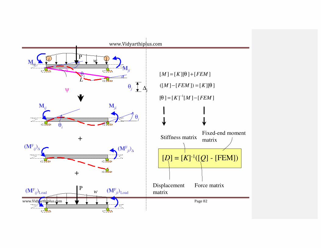
www.Vidyarthiplus.com
www.Vidyarthiplus.com Page 82
i Mij
P w j
θi
L
ψ
Mji
θj
∆j
[M ] = [K ][θ ] + [FEM ]
([M ] − [FEM ]) = [K ][θ ]
[θ ] = [K ]−1[M ] − [FEM ]
(MF
Mij Mji
θj
θi
+ ) F
Stiffness matrix
Fixed-end moment
matrix
ij ∆ (M
+
ji)∆
[D] = [K]-1([Q] - [FEM])
ij)
P (MF ) Displacement Force matrix
(MF
Load w ji
Load matrix

www.Vidyarthiplus.com
www.Vidyarthiplus.com Page 83
12

www.Vidyarthiplus.com
www.Vidyarthiplus.com Page 84
Stiffness Coefficients Derivation: Fixed-End Support
Mi θi
i j
L
Mj
Real beam
M i + M j
L
M i
L/3
M j L
2EI
M i + M j
L M
j
EI
Conjugate beam
EI M L i
θι 2EI
+ ΣM '
= 0 : − ( M i L
)( L
) + ( M j L
)( 2L
) = 0 From (1) and (2);
i 2EI 3 2EI 3
M i = ( 4EI
)θi

www.Vidyarthiplus.com
www.Vidyarthiplus.com Page 85
M i = 2M j − − − (1) L
M L M L M = (
2EI )θ
+ ↑ ΣFy = 0 : θ − ( i ) + ( i
2EI
j
2EI ) = 0 − − − (2) j
L i
13
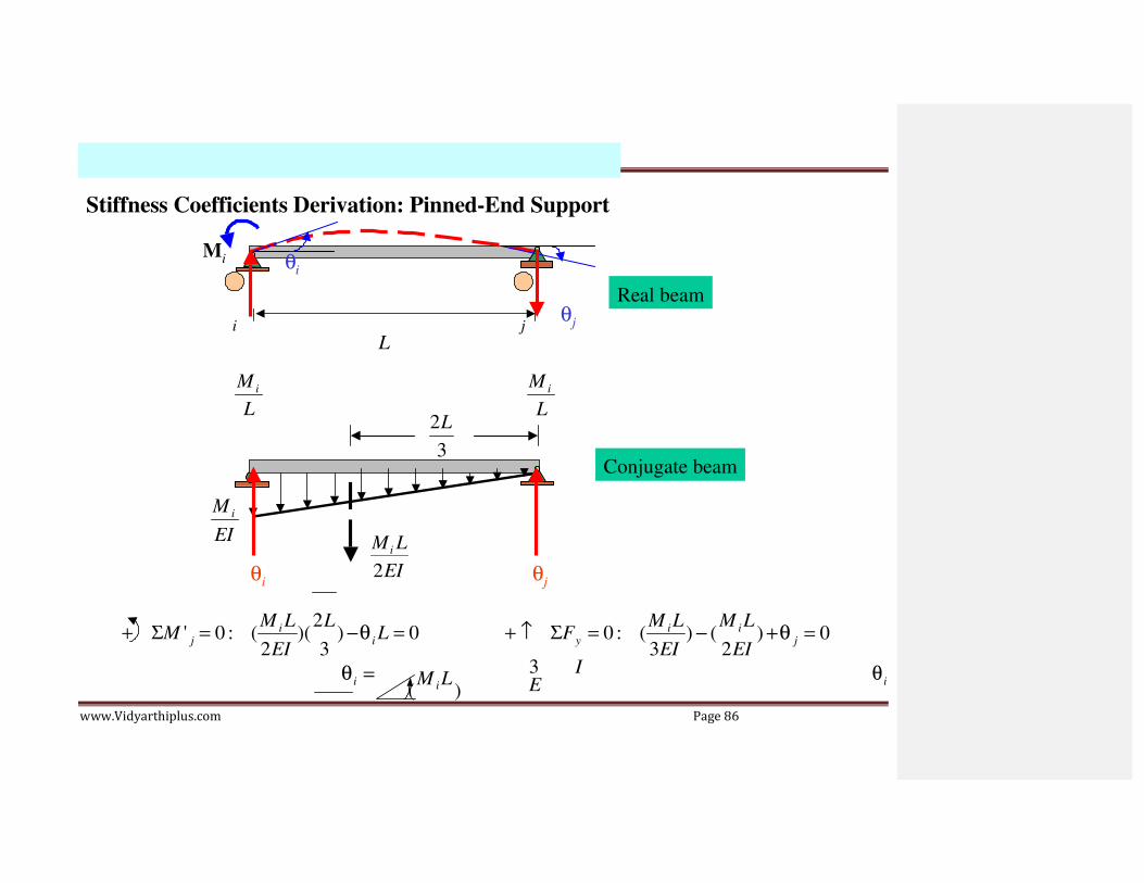
www.Vidyarthiplus.com
www.Vidyarthiplus.com Page 86
θ
Stiffness Coefficients Derivation: Pinned-End Support
Mi i
Real beam
i j θj
L
M i M i
L 2L
3
M i
EI M L
L
Conjugate beam
i
θi 2EI θj
+ ΣM '
= 0 : ( M i L
)( 2L
) − θ
L = 0
+ ↑ ΣF
= 0 : ( M i L
) − ( M i L
) + θ = 0
j 2EI 3
i
y 3EI 2EI
j
θ i =
( M i L
) 3E
I
θ i

www.Vidyarthiplus.com
www.Vidyarthiplus.com Page 87
= 1 = ( M i L
) → 3EI
M i =
3EI L
θ
=
(
−
M
i
L
)
j
6EI
14

www.Vidyarthiplus.com
www.Vidyarthiplus.com Page 88
Fixed end moment : Point Load
P Real beam
A L B
M
Conjugate beam
A B
M M
EI EI
M
EI ML M 2EI
P
PL2
16EI
PL
4EI
M ML EI 2EI
PL2
16EI

www.Vidyarthiplus.com
www.Vidyarthiplus.com Page 89
ML ML
PL2
PL
+ ↑ ΣFy
= 0 :
− 2EI
− 2EI
+ 2 16EI
= 0,
M = 8 15

www.Vidyarthiplus.com
www.Vidyarthiplus.com Page 90
P
PL PL
8 L 8
P P/2
P 2 2
PL/8 P/2
-PL/8 -PL/8
-PL/8
-
-PL/16
-
-PL/16
P
L
/
4
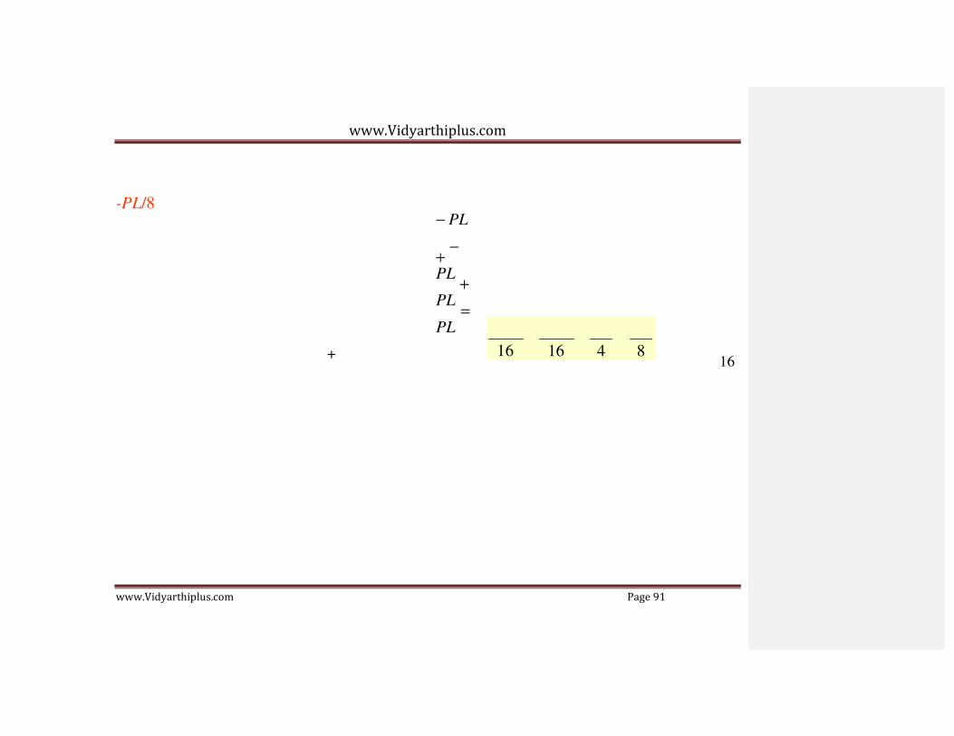
www.Vidyarthiplus.com
www.Vidyarthiplus.com Page 91
-PL/8
− PL
+ −
PL +
PL =
PL
+ 16 16 4 8 16

www.Vidyarthiplus.com
www.Vidyarthiplus.com Page 92
Uniform load
w
Real beam Conjugate beam
A B
A L B
M M M EI EI
M
EI ML M 2EI
wL3
w 24EI
wL2
8EI
M ML EI 2EI
wL3
24EI

www.Vidyarthiplus.com
www.Vidyarthiplus.com Page 93
1
ML ML
wL3
wL2
+ ↑ ΣFy
= 0 :
− 2EI
− 2EI
+ 2 24EI
= 0,
M = 12 7

www.Vidyarthiplus.com
www.Vidyarthiplus.com Page 94
Settlements
Mi = Mj
Real beam Mj
M
Conjugate beam EI
L
M i + M j
M L
A B
∆ ∆ M
M i + M j
L EI
M
EI ML
2EI
M
ML
2EI M
EI
∆
+ ΣM
= 0 : − ∆ − ( ML
)( L
) + ( ML
)( 2L
) = 0,

www.Vidyarthiplus.com
www.Vidyarthiplus.com Page 95
B 2EI
M =
3
6EI∆
L2
2EI 3
18

www.Vidyarthiplus.com
www.Vidyarthiplus.com Page 96
Pin-Supported End Span: Simple Case
P w
B A
4EI θ
L
+ 2EI
θ A
L B
θA
A
L
+ θB
P w
2EI θ
L
B
+ 4EI
θ A
L B
(FEM)AB (FEM)BA
A B
M AB
M BA
= 0 = (4EI / L)θ A
+ (2EI / L)θ B
= 0 = (2EI / L)θ A
+ (4EI / L)θ B
+ (FEM ) AB
+ (FEM ) BA
− − − (1)
− − − (2)
2(2) − (1) :

www.Vidyarthiplus.com
www.Vidyarthiplus.com Page 97
2M BA =
(6EI /
L)θ B
+ 2(FEM ) BA
− (FEM ) BA
M BA
= (3EI / L)θ B
+ (FEM ) BA − (FEM ) BA
2 19

www.Vidyarthiplus.com
www.Vidyarthiplus.com Page 98
AB AB
B
∆
Pin-Supported End Span: With End Couple and Settlement
4EI θ
L
MA
A
+ 2EI
θ A
L B
θA
A
P w
L
P θB
w
B
∆
B
2EI θ
L
F
+ 4EI
θ A
L B
(MF AB)load
(M BA)load
(MF AB)∆
A B (MF
A
BA) ∆
M AB
= M A = 4EI
θ L
A
+ 2EI
θ L
B
+ (M F
)load
+ (M F
)
− − − (1)
M BA

www.Vidyarthiplus.com
www.Vidyarthiplus.com Page 99
BA BA ∆= 2EI
θ L
A
+ 4EI
θ L
B
+ (M F
)load
+ (M F
)
− − − (2)
E lim inate θ by 2(2) − (1) : M
= 3EI
θ
+ [(M F ) −
1 (M
F )
] + 1
(M F
) +
M A
A 2
BA L
B
BA load 2
AB load 2
BA ∆ 2 20

www.Vidyarthiplus.com
www.Vidyarthiplus.com Page 100
Fixed-End Moments
Fixed-End Moments: Loads
P
PL L/2 L/2 PL
8 8
P
L/2 L/2
PL + (
1 )[−(−
PL )] =
3PL
8 2 8 16
wL2
12
wL2
12

www.Vidyarthiplus.com
www.Vidyarthiplus.com Page 101
wL2
12 + (
1 )[−(−
2
wL2
12
)] = wL
2
8 21

www.Vidyarthiplus.com
www.Vidyarthiplus.com Page 102
B P
A B
A B
B
Typical Problem C P1 w 2
A C
B L1 L2
PL P
8
wL2
PL 12
w 8
wL2
12
L L
0
M AB =
4EI θ
L1
+ 2EI
θ L1
0
+ 0 + P
1 L
1
8
M BA = 2EI
θ L
1
+ 4EI
θ L
1
+ 0 − P
1 L
1
8
0 2
M BC = 4EI
θ L2
+ 2EI
θ

www.Vidyarthiplus.com
www.Vidyarthiplus.com Page 103
C
B C
L2
+ 0 +
0
P2 L
2
8 + wL
2
12
2
M CB = 2EI
θ L2
+ 4EI
θ L2
+ 0 + − P2 L2
8 −
wL2
12 22

www.Vidyarthiplus.com
www.Vidyarthiplus.com Page 104
B P
A B
B C
C P1 w 2
A C
B L1 L2
MBA CB MBC
B
M BA = 2EI
θ L1
+ 4EI
θ L1
+ 0 − P1 L1
8
2
M BC = 4EI
θ L2
+ 2EI
θ L2
+ 0 + P2 L2
8 +
wL2
12
+ ΣM B = 0 : CB − M BA − M BC = 0 → Solve for θ B

www.Vidyarthiplus.com
www.Vidyarthiplus.com Page 105
23

www.Vidyarthiplus.com
www.Vidyarthiplus.com Page 106
B P
A B
A B
B C
B C
C P1 w 2
MBA
A C MCB
B MBC
L1 L2
Substitute θB in MAB, MBA, MBC, MCB
M AB
= 4EI
θ L
1
0
+ 2EI
θ L1
0
+ 0 +
P1 L
1
8
M BA =
2EI θ
L1
+ 4EI
θ L
1
+ 0 − P
1 L
1
8
0 2
M BC =
4EI θ
L2
+ 2EI
θ L
2
+ 0 +
0
P2 L
2
8 +
wL2
12
2
M CB =
2EI θ
L2
+ 4EI
θ L
2
+ 0 + − P
2 L
2
8 −
wL2
12

www.Vidyarthiplus.com
www.Vidyarthiplus.com Page 107
24

www.Vidyarthiplus.com
www.Vidyarthiplus.com Page 108
L L
y L BA
MAB
A
P1
MBA
CB P w 2
MBC
MCB
C
1 L2 Cy
By = ByL + ByR
MAB
P1
MBA
A B
MBC
B C P2
MCB
Ay ByL
1
ByR Cy
2

www.Vidyarthiplus.com
www.Vidyarthiplus.com Page 109
25

www.Vidyarthiplus.com
www.Vidyarthiplus.com Page 110
Example of Beams
Example 1
Draw the quantitative shear , bending moment diagrams and qualitative
deflected curve for the beam shown. EI is constant.
10 kN 6 kN/m
A C
4 m
4 m B 6 m

www.Vidyarthiplus.com
www.Vidyarthiplus.com Page 111
27

www.Vidyarthiplus.com
www.Vidyarthiplus.com Page 112
B C
10 kN 6 kN/m
A C
4 m
PL P
4 m B 6 m
2 2
8 PL 8
FEM
wL w 30
wL 20
[M] = [K][Q] + [FEM]
MBA MBC
M AB
= 4EI
θ 8
A
0
+ 2EI
θ 8
B
+ (10)(8)
8
+ ΣM B
B
= 0 :
− M BA − M BC = 0
2
M BA
= 2EI
8
0
θ A
+
4EI θ
8 B
− (10)(8)
8 0
( 4EI
8 +
4EI )θ
6 B
θ
−10 + (6)(6
30
= 2.4
) = 0
M BC
= 4EI
θ + 2EI
θ (6)(62 )
+ B
EI
6 6 30 Substitute θB in the moment equations:

www.Vidyarthiplus.com
www.Vidyarthiplus.com Page 113
M CB
= 2EI
θ 6
B
+ 4EI
θ 6
C
0 (6)(6)
2
− 20
MAB = 10.6 kN•m,
MBA = - 8.8 kN•m,
MBC = 8.8 kN•m
MCB = -10 kN•m 28

www.Vidyarthiplus.com
www.Vidyarthiplus.com Page 114
10 kN 6 kN/m 8.8 kN•m
10.6 kN•m
A C 8.8 kN•m
10 kN•m
4 m
4 m B 6 m
MAB = 10.6 kN•m,
MBA = - 8.8 kN•m,
MBC = 8.8 kN•m
MCB= -10 kN•m
2 m
10.6 kN•m
10 kN
A B
8.8 kN•m B
8.8 kN•m
18 kN
6 kN/m
10 kN•m
Ay = 5.23 kN ByL = 4.78 kN ByR
= 5.8 kN Cy = 12.2 kN

www.Vidyarthiplus.com
www.Vidyarthiplus.com Page 115
29

www.Vidyarthiplus.com
www.Vidyarthiplus.com Page 116
10 kN 6 kN/m
10.6 kN•m A C
10 kN•m
5.23 kN
4 m
4 m B 6 m
12.2 kN
V (kN)
5.23
+
4.78 + 5.8 = 10.58 kN
5.8
+
- -
- 4.78
x (m)
M
(kN•m)
10.3
- -
-10.6
-8.8
+
θ B
=
-
2.4

www.Vidyarthiplus.com
www.Vidyarthiplus.com Page 117
EI
-12.2
x (m)
-10 Deflected shape x (m)
30

www.Vidyarthiplus.com
www.Vidyarthiplus.com Page 118
Example 2
Draw the quantitative shear , bending moment diagrams and qualitative
deflected curve for the beam shown. EI is constant.
10 kN 6 kN/m
A C
4 m
4 m B 6 m

www.Vidyarthiplus.com
www.Vidyarthiplus.com Page 119
31

www.Vidyarthiplus.com
www.Vidyarthiplus.com Page 120
10 kN 6 kN/m
A C
PL P 8
4 m
4 m
PL
8
B 6 m
wL2 w 30
FEM
wL2 20
[M] = [K][Q] + [FEM] 10
0
M AB =
4EI θ
8 A
+ 2EI
θ 8
B +
(10)(8) 8
− − − (1)
M BA
= 2EI
θ 8
A
+ 4EI
θ 8
B
− (10)(8)
8
10
− − − (2)
M BC =
4EI θ
6 B
+ 2EI
θ 6
C
0 (6)(62 ) +
30
− − − (3)
2(2)
− (1)
:
M CB
2M BA
= 2EI
θ 6
B
= 6EI
θ 8
B
3EI

www.Vidyarthiplus.com
www.Vidyarthiplus.com Page 121
+ 4EI
θ 6
C
− 30
0 (6)(6)2
− 20
− − − (4)
M BA = θ B
− 15 8
− − − (5) 32

www.Vidyarthiplus.com
www.Vidyarthiplus.com Page 122
2
2
MBA MBC
M BC
= 4EI
θ 6
B
B
+ (6)(6 )
30
− − − (3)
Substitute θA and θB in (5), (3) and (4):
M CB
= 2EI
θ 6
B
− (6)(6)
20
− − − (4)
MBA = - 12.19 kN•m
MBC = 12.19 kN•m
M BA =
3EI θ
8 B
− 15
− − − (5)
MCB = - 8.30 kN•m
+ ΣM B = 0 : − M
BA − M
BC = 0
( 3EI
8 +
4EI 6
)θ B
− 15 + (6)(62 )
= 0 30
− − − (6)
θ B
= 7.488
EI
Substitute θ B
in (1) :
0 = 4EI
θ 8
A
+ 2EI
θ

www.Vidyarthiplus.com
www.Vidyarthiplus.com Page 123
8 B
−10
θ A = − 23.74
EI 33

www.Vidyarthiplus.com
www.Vidyarthiplus.com Page 124
10 kN 6 kN/m 12.19 kN•m
A C 12.19 kN•m
8.30 kN•m
4 m
4 m B 6 m
MBA = - 12.19 kN•m, MBC = 12.19 kN•m, MCB = - 8.30 kN•m
10 kN
A B
B 12.19 kN•m
2 m
18 kN
6 kN/m
C
Ay = 3.48 kN
ByL
12.19 kN•m
= 6.52 kN
ByR
= 6.65 kN
8.30 kN•m
Cy = 11.35 kN

www.Vidyarthiplus.com
www.Vidyarthiplus.com Page 125
34

www.Vidyarthiplus.com
www.Vidyarthiplus.com Page 126
10 kN 6 kN/m
A C
3.48 kN
4 m
4 m B 6 m
11.35 kN
6.52 + 6.65 = 13.17 kN
V (kN)
3.48 6.65
x (m)
M
- 6.52
14
-11.35
(kN•m) x (m)
-8.3 -12.2
θ B =

www.Vidyarthiplus.com
www.Vidyarthiplus.com Page 127
7.49 E I Deflected shape x (m)
θ A = − 23.74
EI 35

www.Vidyarthiplus.com
www.Vidyarthiplus.com Page 128
Example 3
Draw the quantitative shear , bending moment diagrams and qualitative
deflected curve for the beam shown. EI is constant.
10 kN 4 kN/m
A C
2EI 3EI B
4 m
4 m
6 m

www.Vidyarthiplus.com
www.Vidyarthiplus.com Page 129
36

www.Vidyarthiplus.com
www.Vidyarthiplus.com Page 130
A B
2
10 kN 4 kN/m
A C
2EI 3EI
(10)(8)/8 4 m
(10)(8)/8
4 m
B (4)(62)/12 (4)(62)/12
6 m
0 10
M = 4(2EI )
θ + 2(2EI )
θ + (10)(8)
− − − (1) AB 8
A 8
B 8 10
M BA =
2(2EI ) θ +
4(2EI ) θ −
(10)(8)
− − − (2) 8 8 15 8
2(2) − (1) :
2
M BA = 3(2EI )
θ 8
B
− (3 / 2)(10)(8)
8
− − − (2a)
M BC
= 4(3EI )
θ 6
B
+ (4)(6 )
12
12
− − − (3)

www.Vidyarthiplus.com
www.Vidyarthiplus.com Page 131
37

www.Vidyarthiplus.com
www.Vidyarthiplus.com Page 132
2
10 kN 4 kN/m
A C
2EI 3EI
4 m (3/2)(10)(8)/8 B
4 m
(4)(62)/12 (4)(62)/12
6 m
M BA
= 3(2EI )
θ 8
B
15
− (3 / 2)(10)(8)
8
− − − (2a)
M BC
= 4(3EI )
θ 6
B
+ (4)(6 )
12
12
− − − (3)
− M BA − M BC = 0 : 2.75EIθ B
θ B
= −12 + 15 = 3
= 1.091/ EI
3(2
) 1.091
M BA = EI
( 8 EI
) −15 = −14.18 kN • m
4(3
) 1.091
M BC = EI
( 6 EI

www.Vidyarthiplus.com
www.Vidyarthiplus.com Page 133
) −12 = 14.18 kN • m
M CB = 2(3EI )
θ 6
B
−12 = −10.91 kN • m 38

www.Vidyarthiplus.com
www.Vidyarthiplus.com Page 134
10 kN 4 kN/m
A C 10.91
2EI
4 m
14.18 B
4 m
14.18
6 m
3EI
MBA = - 14.18 kN•m, MBC = 14.18 kN•m, MCB = -10.91 kN•m
10 kN
A B
14.18 kN•m
140.18 kN•m
24 kN
C
10.91 kN•m
Ay = 3.23 kN ByL = 6.73 kN ByR = 12.55 kN Cy = 11.46 kN

www.Vidyarthiplus.com
www.Vidyarthiplus.com Page 135
39

www.Vidyarthiplus.com
www.Vidyarthiplus.com Page 136
10 kN 4 kN/m
A C
2EI 3EI 10.91 kN•m
3.23 kN
4 m
4 m
B
6 m
11.46 kN
V (kN)
M
(kN•m)
3.23 +
6.77 + 12.55 = 19.32 kN
12.55
2.86
+
- - -6.73
12.91
5.53
+ +
- -
x (m)
-11.46
x (m)
-10.91
-14.18
θB = 1.091/EI

www.Vidyarthiplus.com
www.Vidyarthiplus.com Page 137
Deflected shape x (m)
40

www.Vidyarthiplus.com
www.Vidyarthiplus.com Page 138
Example 4
Draw the quantitative shear , bending moment diagrams and qualitative
deflected curve for the beam shown. EI is constant.
10 kN 12 kN•m 4 kN/m
A C
2EI 3EI B
4 m
4 m
6 m

www.Vidyarthiplus.com
www.Vidyarthiplus.com Page 139
41

www.Vidyarthiplus.com
www.Vidyarthiplus.com Page 140
10 kN 12 kN•m
4 kN/m
A C 2EI 3EI
4 m
1.5PL/8 = 15 B
4 m
wL2/12 = 12 wL2/12 = 12
6 m
M = 3(2EI )
θ
− 15
− − − (1) 0 -3.273/EI
BA 8
B
4(3EI )
M AB = 4(2EI )
θ 8
A
+ 2(3EI )
θ 8
B
+ (10)(8)
8 M BC = θ B + 12
6 − − − (2)
θ = − 7.21
A EI
M CB = 2(3EI )
θ 6
B
−12
− − − (3)
M BA
= 0.75EI (−
3.273
) −15 = −17.45 kN • m
MBA
MBA
12 kN•m
M BC
EI
= 2EI (− 3.273
) + 12 = 5.45 kN • m EI
B MBC
MBC
M CB = EI (− 3.273
) − 12 = −15.27 kN • m EI
Jo int B : − M BA − M BC − 12 = 0
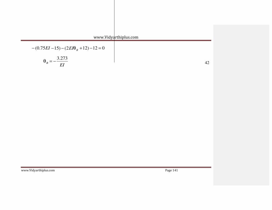
www.Vidyarthiplus.com
www.Vidyarthiplus.com Page 141
− (0.75EI − 15) − (2EIθ B + 12) − 12 = 0
θ = − 3.273
B EI
42

www.Vidyarthiplus.com
www.Vidyarthiplus.com Page 142
m
M BA
= 0.75EI (− 3.273
EI
) −15 = −17.45 kN • m
M BC
= 2EI (−
3.273
EI
) + 12 = 5.45 kN • m
M CB
= EI (− 3.273
EI
) − 12 = −15.27 kN • m
10 kN
A B
2.82 kN
17.45 kN•m
7.18 kN
5.45 kN•
24 kN
10.36 kN
4 kN/m
15.27 kN•m C
13.64 kN
10 kN 12 kN•m 4 kN/m
A C 15.27 kN•m

www.Vidyarthiplus.com
www.Vidyarthiplus.com Page 143
B 2.82 kN
17.54 kN 13.64 kN
43

www.Vidyarthiplus.com
www.Vidyarthiplus.com Page 144
10 kN 12 kN•m
4 kN/m
A C
2EI 3EI 15.27 kN•m
V (kN)
2.82 kN
4 m
2.82
4 m
B 17.54 kN
6 m
10.36
13.64 kN θ = − 7.21
A EI
θ = − 3.273
B EI
M
(kN•m)
+ -
-7.18
11.28
+
+
+
- -5.45
3.41 m
-
7.98
-
x (m)
-13.64
x (m)
-17.45 -15.27

www.Vidyarthiplus.com
www.Vidyarthiplus.com Page 145
Deflected shape x (m)
θ A =
− 7.21
EI
θ B =
3.273
EI 44

www.Vidyarthiplus.com
www.Vidyarthiplus.com Page 146
Example 5
Draw the quantitative shear, bending moment diagrams, and qualitative
deflected curve for the beam shown. Support B settles 10 mm, and EI is
constant. Take E = 200 GPa, I = 200x106 mm4.
12 kN•m 10 kN 6 kN/m
B
A C
2EI 3EI
10 mm 4 m 4 m 6 m

www.Vidyarthiplus.com
www.Vidyarthiplus.com Page 147
45

www.Vidyarthiplus.com
www.Vidyarthiplus.com Page 148
B
C
12 kN•m 10 kN 6 kN/m
B
A C
2EI 3EI
10 mm
6EI∆ A
L2
4 m
∆
4 m
6EI∆
L2
6 m
6EI∆
L2
∆
6EI∆ L
2
PL
8
-12
M =
P
4(2EI ) θ
PL
8
+ 2(2EI )
θ
wL2
30
[FEM]load
+ 6(2EI )(0.01)
+ (10)(8)
w
− − − (1)
wL2
30
AB 8
A 8
B 8
2 8
M = 2(2EI )
θ + 4(2EI )
θ + 6(2EI )(0.01)
− (10)(8)
− − − (2) BA 8
A 8 82 8
0 2
M = 4(3EI )
θ + 2(3EI )
θ − 6(3EI )(0.01)
+ (6)(6 ) − − − (3)

www.Vidyarthiplus.com
www.Vidyarthiplus.com Page 149
0BC
6 B
6 62
30 2
M = 2(3EI )
θ + 4(3EI )
θ − 6(3EI )(0.01)
− (6)(6)
− − − (4) CB 6
B 6
C 62 30 46

www.Vidyarthiplus.com
www.Vidyarthiplus.com Page 150
12 kN•m 10 kN 6 kN/m
B
A C
2EI 3EI
10 mm 4 m
M = 4(2EI )
θ
4 m
+ 2(2EI )
θ
6 m
+ 6(2EI )(0.01)
+ (10)(8)
− − − (1) AB
8 A
8 B
82
8
M = 2(2EI )
θ + 4(2EI )
θ + 6(2EI )(0.01)
− (10)(8)
− − − (2) BA
8 A
8 B
82
8
Substitute EI = (200x106 kPa)(200x10-6 m4) = 200x200 kN• m2 :
M AB
M BA
= 4(2EI )
θ 8
A
= 2(2EI )
θ 8
A
+ 2(2EI )
θ 8
B
+ 4(2EI )
θ 8
B
+ 75 + 10
+ 75 − 10
16.5
− − − (1)
− − − (2)
2(2) − (1) :
2

www.Vidyarthiplus.com
www.Vidyarthiplus.com Page 151
M BA
= 3(2
EI )
θ 8
B
+ 75 − (75 /
2) −10 −
(10 / 2) −12
/ 2 − − −
(2a)
47

www.Vidyarthiplus.com
www.Vidyarthiplus.com Page 152
12 kN•m 10 kN 6 kN/m
B
A C
2EI 3EI
10 mm 4 m 4 m 6 m
MBA = (3/4)(2EI)θB + 16.5
MBC = (4/6)(3EI)θB - 192.8
+ ΣMB = 0: - MBA - MBC = 0 (3/4 + 2)EIθB + 16.5 - 192.8 = 0
MBA MBC
B
θB = 64.109/ EI
Substitute θB in (1): θA = -129.06/EI
Substitute θA and θB in (5), (3), (4):
MBA = 64.58 kN•m,
MBC = -64.58 kN•m

www.Vidyarthiplus.com
www.Vidyarthiplus.com Page 153
MCB = -146.69
kN•m
48

www.Vidyarthiplus.com
www.Vidyarthiplus.com Page 154
12 kN•m 10 kN 6 kN/m
B
A C
64.58 kN•m 64.58 kN•m
146.69 kN•m
4 m 4 m 6 m
MBA = 64.58 kN•m,
MBC = -64.58 kN•m
MCB = -146.69 kN•m
2 m
12 kN•m
10 kN
64.58 kN•m
64.58 kN•m
18 kN
6 kN/m
A B 146.69 kN•m
B C
Ay
= 11.57 kN ByL = -1.57 kN ByR = -29.21 kN Cy = 47.21 kN

www.Vidyarthiplus.com
www.Vidyarthiplus.com Page 155
49

www.Vidyarthiplus.com
www.Vidyarthiplus.com Page 156
12 kN•m 10 kN 6 kN/m
A C
2EI 3EI
146.69 kN•m
11.57 kN
4 m
4 m
B
6 m
47.21 kN
θA = -129.06/EI 1.57 + 29.21 = 30.78 kN θ = 64.109/ EI
V (kN)
11.57 1.57
+
- -29.21
58.29 64.58
B
x (m)
-47.21
M 12
+ (kN•m)
x (m)
-
-146.69

www.Vidyarthiplus.com
www.Vidyarthiplus.com Page 157
Deflected shape x (m)
10 mm
θA = -129.06/EI θB = 64.109/ EI 50

www.Vidyarthiplus.com
www.Vidyarthiplus.com Page 158
Example 6
For the beam shown, support A settles 10 mm downward, use the slope-deflection
method to
(a)Determine all the slopes at supports
(b)Determine all the reactions at supports
(c)Draw its quantitative shear, bending moment diagrams, and qualitative
deflected shape. (3 points)
Take E= 200 GPa, I = 50(106) mm4.
6 kN/m 12 kN•m
B A
2EI C 1.5EI 10 mm
3 m 3 m

www.Vidyarthiplus.com
www.Vidyarthiplus.com Page 159
51

www.Vidyarthiplus.com
www.Vidyarthiplus.com Page 160
M
M
A
6 kN/m 12 kN•m
B A
2EI C 1.5EI 10 mm
3 m 3 m
6(32 )
12
= 4.5
C
6 kN/m
F w
4.5
6(1.5 × 200 × 50)(0.01) C
32
= 100 kN • m
0.01 m
F ∆
A
100 kN • m
M CB = 4(2EI )
θ 3
C
− − − (1)
M CA
12
= 4(1.5EI )
θ 3
C
+ 2(1.5EI )
θ 3
A
+ 4.5 + 100
− − − (2)
M AC = 2(1.5EI )
θ 3 C
+
4(1.5EI ) θ

www.Vidyarthiplus.com
www.Vidyarthiplus.com Page 161
C
3 A
− 4.5 + 100
− − − (3)
2(2) − (2) :
M CA
= 3(1.5EI )
θ
+ 3(4.5)
+ 100
+ 12
− − − (2a) 2 3 2 2 2 52

www.Vidyarthiplus.com
www.Vidyarthiplus.com Page 162
6 kN/m 12 kN•m
B A
2EI C 1.5EI 10 mm
3 m 3 m
M CB = 4(2EI )
θ 3
C
− − − (1)
M = 3(1.5EI )
θ
+ 3(4.5)
+ 100
+ 12
− − − (2a) CA
3 C
2 2 2
MCB MCA
• Equilibrium equation:
M CB + M
CA = 0
(8 + 4.5)EI θ
+
3(4.5) +
100 +
12 =
C 3
C 2 2 2
0
θC
=
−15.06
EI
= −0.0015 rad
Substitute θC in eq.(3)
12 =
2(1.5EI ) ( −15.06
) + 4(1.5EI )
θ
− 4.5 + 100
− − − (3)

www.Vidyarthiplus.com
www.Vidyarthiplus.com Page 163
3 EI 3 A
− 34.22 θ
A =
EI = −0.0034 rad
53

www.Vidyarthiplus.com
www.Vidyarthiplus.com Page 164
6 kN/m 12 kN•m
B A
2EI C 1.5EI 10 mm
3 m 3 m
θ C
= −15.06
EI
= −0.0015 rad
θ A
= − 34.22
EI
= −0.0034 rad
M = 2(2EI )
θ = 2(2EI )
( − 15.06
) = −20.08 kN • m
BC 3
C 3 EI
M = 4(2EI )
θ = 4(2EI )
( −15.06
) = −40.16 kN • m
CB 3
C 3
20.08 kN•m
EI
40.16 kN•m B C
20.08 kN 40.16 + 20.08
3
40.16 kN•m
= 20.08 kN
18 kN
6 kN/m

www.Vidyarthiplus.com
www.Vidyarthiplus.com Page 165
12 kN•m C
26.39 kN A
8.39 kN 54

www.Vidyarthiplus.com
www.Vidyarthiplus.com Page 166
6 kN/m 12 kN•m
θC = −0.0015 rad B A
θ A = −0.0034 rad 2EI C 1.5EI 10 mm
20.08 kN•m
3 m 3 m
40.16 kN•m B C
20.08 kN
20.08 kN
40.16 kN•m
6 kN/m 12 kN•m
V (kN)
M (kN•m)
-
-20.08
20.08
C 26.39 kN
26.39
+
A 8.39 kN
8.39 x (m)
12 x (m)

www.Vidyarthiplus.com
www.Vidyarthiplus.com Page 167
Deflected shape -40.16
θC
= 0.0015 rad
x (m)
θ A = 0.0034 rad 55

www.Vidyarthiplus.com
www.Vidyarthiplus.com Page 168
Example 7
For the beam shown, support A settles 10 mm downward, use the
slope-deflection method to
(a)Determine all the slopes at supports
(b)Determine all the reactions at supports
(c)Draw its quantitative shear, bending moment diagrams, and qualitative
deflected shape.
Take E= 200 GPa, I = 50(106) mm4.
6 kN/m 12 kN•m
B A
2EI C 1.5EI 10 mm
3 m 3 m

www.Vidyarthiplus.com
www.Vidyarthiplus.com Page 169
56

www.Vidyarthiplus.com
www.Vidyarthiplus.com Page 170
6 kN/m 12 kN•m
B A
2EI C 1.5EI 10 mm
3 m 3 m
B
6(2EI )∆C =
4EI∆C
C EI∆C
∆C
4EI∆C
3
C
∆C
6 kN/m
6(1.5EI )∆C = EI∆
2
32 3 4.5
C
6(3 )
A 12
= 4.5
M BC
= 2(2EI )
θ 3
C
− 4EI
∆ 3
C
100 C
− − − (1)
0.01 m
6(1.5 × 200 ×
50)(0.01)
32
M CB =
4(2EI ) θ
3 C
− 4EI
∆ 3
C
− − − (2) A = 100 kN • m
M CA
= 4(1.5EI )
θ 3
C
+ 2(1.5EI )
θ 3
A
+ EI∆C
+ 4.5 + 100 − −(3)

www.Vidyarthiplus.com
www.Vidyarthiplus.com Page 171
12
M AC
= 2(1.5EI )
θ 3
C
+ 4(1.5EI )
θ 3
A
+ EI∆C
− 4.5 + 100 − −(4)
2(3) − (4)
2
: M CA
= 3(1.5EI )
θ 3
C
+ EI 2
∆C
+ 3(4.5)
2 +
100 2
+ 12 2
− − − (3a) 57
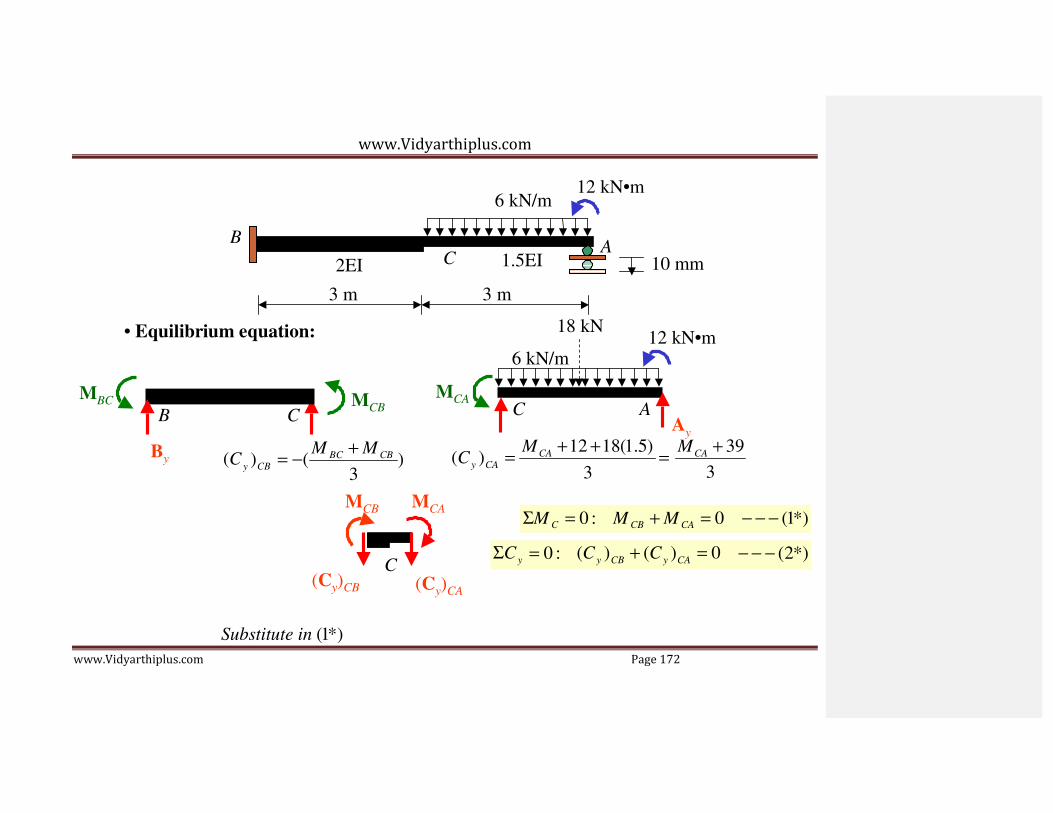
www.Vidyarthiplus.com
www.Vidyarthiplus.com Page 172
y
6 kN/m 12 kN•m
B A
2EI C 1.5EI 10 mm
• Equilibrium equation:
3 m 3 m
18 kN
12 kN•m
MBC
B C
MCB
MCA
6 kN/m
C A A
y
By (C
)CB = −(
M BC + M CB ) 3
MCB MCA
(C y
)CA
= M
CA + 12 + 18(1.5)
= 3
M CA
+ 39
3
ΣM C = 0 : M CB + M CA = 0 − − − (1*)
(Cy)CB
C
(Cy)CA
ΣC y = 0 : (C
y )
CB + (C
y )
CA = 0 − − − (2*)
Substitute in (1*)
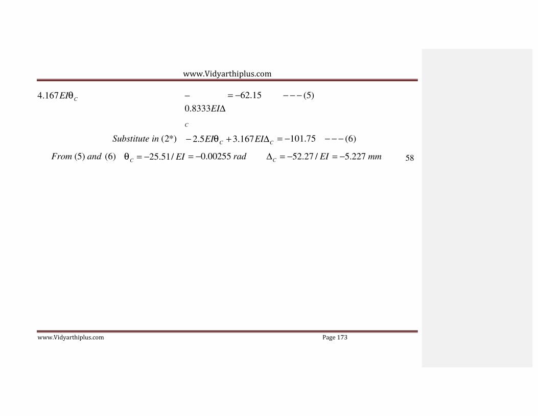
www.Vidyarthiplus.com
www.Vidyarthiplus.com Page 173
4.167 EIθC −
0.8333EI∆
C
= −62.15 − − − (5)
Substitute in (2*) − 2.5EIθC + 3.167 EI∆C = −101.75 − − − (6)
From (5) and (6) θC
= −25.51 / EI = −0.00255 rad ∆C
= −52.27 / EI = −5.227 mm 58

www.Vidyarthiplus.com
www.Vidyarthiplus.com Page 174
6 kN/m 12 kN•m
B A
2EI C 1.5EI 10 mm
• Solve equation
3 m 3 m
θ C
= − 25.51
= −0.00255 rad EI
Substitute θC and ∆C in (1), (2) and (3a)
∆C
=
− 52.27
EI
= −5.227 mm M BC
M CB
= 35.68 kN • m
= 1.67 kN • m
Substitute θC and ∆C in (4) M CA = −1.67 kN • m
θ A
= − 2.86
EI
= −0.000286 rad
6 kN/m
12 kN•m
35.68 kN•m B A
B
y
=
1
8
− 5.55

www.Vidyarthiplus.com
www.Vidyarthiplus.com Page 175
2EI C 1.5
EI
Ay
=
18(
4.5)
−12
− 35.6
8
= 12.45 kN 3 m 3 m 6
= 5.55 kN
59

www.Vidyarthiplus.com
www.Vidyarthiplus.com Page 176
6 kN/m 12 kN•m
35.68 kN•m B A
2EI C 1.5EI 10 mm 12.45 kN
3 m 3 m 5.55 kN
V (kN) θ
C = −0.00255 rad
∆C = −5.227 mm
12.45
+
0.925 m
x (m)
θ A
= −0.000286 rad
M (kN•m)
-
1.67
14.57
+
-5.55
12
x (m)
Deflected shape
-35.68
∆C
= 5.227 mm

www.Vidyarthiplus.com
www.Vidyarthiplus.com Page 177
x (m)
θC = 0.00255 rad
θ A
= 0.000286 rad 60

www.Vidyarthiplus.com
www.Vidyarthiplus.com Page 178
Example of Frame: No Sidesway

www.Vidyarthiplus.com
www.Vidyarthiplus.com Page 179
61

www.Vidyarthiplus.com
www.Vidyarthiplus.com Page 180
Example 6
For the frame shown, use the slope-deflection method to
(a) Determine the end moments of each member and reactions at supports
(b) Draw the quantitative bending moment diagram, and also draw the
qualitative deflected shape of the entire frame.
10 kN 12 kN/m
B 3 m
40 kN
3EI
C
2EI
3 m A
1 m 6 m

www.Vidyarthiplus.com
www.Vidyarthiplus.com Page 181
62

www.Vidyarthiplus.com
www.Vidyarthiplus.com Page 182
10 kN 36/2 = 18 12 kN/m
C
• Equilibrium equations
10
3 m
40 kN
3 m
B 36 PL/8 = 30
3EI
2EI (wL2/12 ) =36
MBA
MBC
A PL/8 = 30 10 − M BA
− M BC
= 0 − − − (1*)
1 m 6 m
Substitute (2) and (3) in (1*)
• Slope-Deflection Equations 10 − 3EIθ B + 30 − 54 = 0
M AB
= 2(3EI )
θ 6
B
+ 30
− − − (1)
θ B
= −14
= (3EI )
− 4.667
EI
M BA
= 4(3EI )
θ 6
B
− 30
− − − (2)
Substituteθ B
= − 4.667
EI
in (1) to (3)
M BC
= 3(2EI )
θ 6 B

www.Vidyarthiplus.com
www.Vidyarthiplus.com Page 183
+ 36 +
18
− − − (3)
M AB
M BA
M BC
= 25.33
kN • m
=
−39.33
kN • m
= 49.33
kN • m
63

www.Vidyarthiplus.com
www.Vidyarthiplus.com Page 184
θ
10 kN
B 3 m
40 kN
49.33
39.33
3EI
2EI
M
12 kN/m
C
= 25.33 kN•m
10 -49.33
27.7
-39.3
20.58
3 m
AB
MBA = -39.33 kN•m
A 25.33
M = 49.33 kN•m
-25.33
1 m
B 49.33
6 m
BC
12 kN/m
C
Bending moment diagram
θB
B 39.33
27.78 kN
θB = -4.667/EI B
40 kN

www.Vidyarthiplus.com
www.Vidyarthiplus.com Page 185
A 17.67 kN
25.33
Deflected curve 64

www.Vidyarthiplus.com
www.Vidyarthiplus.com Page 186
Example 7
Draw the quantitative shear, bending moment diagrams and qualitative
deflected curve for the frame shown. E = 200 GPa.
25 kN
B
240(106) mm4 C
5 kN/m
E 180(106)
5 m
120(106) mm4
60(106) mm4
A
3 m
D
3 m 4 m

www.Vidyarthiplus.com
www.Vidyarthiplus.com Page 187
65

www.Vidyarthiplus.com
www.Vidyarthiplus.com Page 188
θ
25 kN
PL/8 = 18.75 18.75 B
5 kN/m
E
5 m
240(106) mm4 C
120(106) mm4
180(106)
6.667+ 3.333
60(106) mm4
(wL2/12 ) = 6.667
A
3 m
D
3 m 4 m
M AB
M BA
= 4(2EI )
5
= 2(2EI )
0 θ
A +
0
θ A
+
2(2EI ) θ
5 B
4(2EI ) B
8 16
M BA
+ M BC
= 0
8 5
M = 4(4EI )
θ 5
+ 2(4EI )
θ
+ 18.75
( + )EIθ B
5 6 + ( )EIθ
C
6 = −18.75 − − − (1)
BC 6
B 6
C M
CB + M CD
+ M CE
= 0
M = 2(4EI )
θ
+ 4(4EI )
θ
− 18.75
8 16 3 9 CB
6 B
6 C ( )EIθ
B + (
6 6 + + )EIθ
C
5 4 = 8.75 − − − (2)

www.Vidyarthiplus.com
www.Vidyarthiplus.com Page 189
M CD =
3(EI ) θ
5 C
3(3EI )
From (1) and
(2) :
θ = − 5.29
θ B
EI C
= 2.86 EI
M CE = θC
+ 10 66 4

www.Vidyarthiplus.com
www.Vidyarthiplus.com Page 190
Substitute θB
= -1.11/EI, θc
= -20.59/EI below
M AB
= 4(2EI )
θ 5
0
+ 2(2EI )
θ A
5 B
MAB = −4.23 kN•m
M = 2(2EI )
θ 0
+ 4(2EI )
θ
MBA = −8.46 kN•m BA
M BC
M CB
M
5 A
= 4(4EI )
θ 6
B
= 2(4EI )
θ 6
B
= 3(EI )
θ
5 B
+ 2(4EI )
θ 6
C
+ 4(4EI )
θ 6
C
+ 18.75
− 18.75
MBC = 8.46 kN•m
MCB = −18.18 kN•m
MCD = 1.72 kN•m CD
5 C
M CE =
3(3EI ) θ
4 C
+ 10
MCE = 16.44 kN•m

www.Vidyarthiplus.com
www.Vidyarthiplus.com Page 191
67
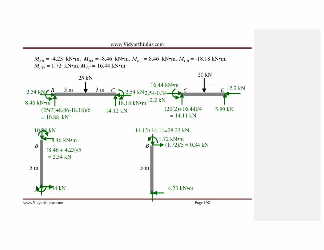
www.Vidyarthiplus.com
www.Vidyarthiplus.com Page 192
MAB = -4.23 kN•m, MBA = -8.46 kN•m, MBC = 8.46 kN•m, MCB = -18.18 kN•m, MCD = 1.72 kN•m, MCE = 16.44 kN•m
2.54 kN
25 kN
B 3 m 3 m C
16.44 kN•m
2.54 kN 2.54-0.34
20 kN
C E
2.2 kN
8.46 kN•m 18.18 kN•m=2.2 kN
(25(3)+8.46-18.18)/6
= 10.88 kN 14.12 kN (20(2)+16.44)/4
= 14.11 kN 5.89 kN
10.88 kN
8.46 kN•m
14.12+14.11=28.23 kN
1.72 kN•m
B
5 m
(8.46 + 4.23)/5
= 2.54 kN
B
5 m
(1.72)/5 = 0.34 kN
A 2.54 kN
4.23 kN•m

www.Vidyarthiplus.com
www.Vidyarthiplus.com Page 193
A 0.34 kN
10.88 kN 28.23 kN 68

www.Vidyarthiplus.com
www.Vidyarthiplus.com Page 194
10.88
+
-2.54
-
-
-14.12
14.11
+
2.82 m
+
1.18 m
-
-5.89
0.78 m
-8.46 -
+
-8.46
24.18
1.29 m 2.33 m
1.72
- -
-18.18 -16.44
3.46
+
1.18 m
-2.54
0.34
4.23
1.67m +
Moment diagram
Shear diagram
0.78 m
1.29 m
2.33 m
θB = −5.29/EI
1.18 m

www.Vidyarthiplus.com
www.Vidyarthiplus.com Page 195
1.67m θC = 2.86/EI
Deflected curve

www.Vidyarthiplus.com
www.Vidyarthiplus.com Page 196
Example 8
Determine the moments at each joint of the frame and draw the quantitative
bending moment diagrams and qualitative deflected curve . The joints at A and
D are fixed and joint C is assumed pin-connected. EI is constant for each member
1 m
3m
B C
10 kN
3 m
A D
71

www.Vidyarthiplus.com
www.Vidyarthiplus.com Page 197
1 m
• Overview
B C
10 kN
• Unknowns
θ
and ∆ B
3 m
MAB MDC
• Boundary Conditions
θA = θD = 0
A Ax
3m
D Dx
• Equilibrium Conditions
- Joint B Ay
Dy
B
MBA
MBC
ΣM B = 0 : M BA + M BC = 0 − − − (1*)
- Entire Frame

www.Vidyarthiplus.com
www.Vidyarthiplus.com Page 198
+
→ ΣFx
= 0 :
10 − Ax − Dx = 0
− − − (2*) 72

www.Vidyarthiplus.com
www.Vidyarthiplus.com Page 199
∆
1 m
3 m
∆ ∆
(0.375EI∆)∆
B C
10 kN
(5.625)load
(0.375EI∆)∆
10 kN
MAB
B
4 m
C
4 m
(1.875)load
A (0.375EI∆)
3m
(1/2)(0.375EI∆)∆ (0.375EI∆)∆
D
A Ax
D Dx
• Slope-Deflection Equations
5.625 0.375EI∆ 2
MBA MDC
M AB = 2(EI )
θ 4
B +
10(3)(1
42
) +
6EI∆ 42
− − − (1) + ΣM B = 0 :
5.625 0.375EI∆ A = (M AB + M BA )
M BA
= 4(EI )
θ 4
B
10(32 )(1) − +
42
6EI∆
42
− − − (2)
x
Ax = 0.375EIθ B
4
+ 0.1875EI∆ + 1.563 − − − (5) M BC
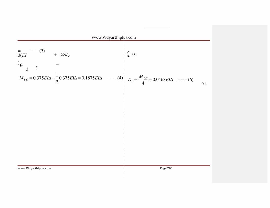
www.Vidyarthiplus.com
www.Vidyarthiplus.com Page 200
= 3(EI
) θ
3 B
− − − (3)
+ ΣM C
= 0 :
M DC = 0.375EI∆ − 1
0.375EI∆ = 0.1875EI∆ 2
− − − (4)
Dx =
M DC
4
= 0.0468EI∆
− − − (6) 73
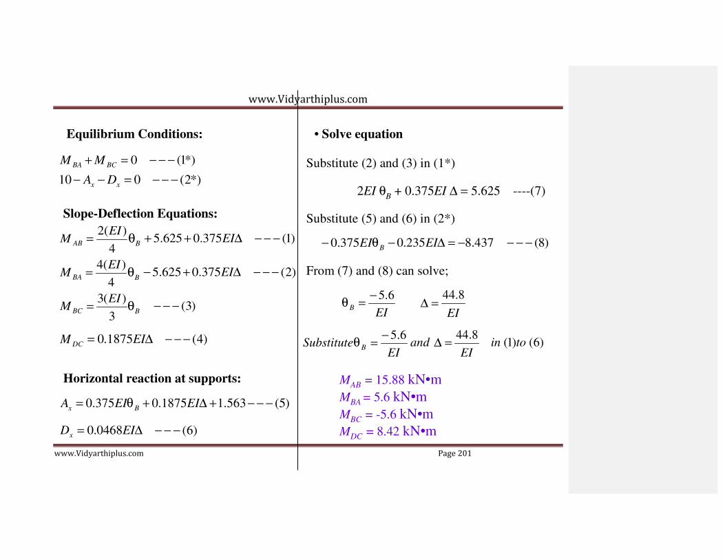
www.Vidyarthiplus.com
www.Vidyarthiplus.com Page 201
Equilibrium Conditions: • Solve equation
M BA + M BC = 0
10 − Ax − Dx = 0
− − − (1*)
− − − (2*)
Substitute (2) and (3) in (1*)
2EI θB + 0.375EI ∆ = 5.625 ----(7)
Slope-Deflection Equations:
Substitute (5) and (6) in (2*)
M AB = 2(EI )
θ 4
B
+ 5.625 + 0.375EI∆
− − − (1)
− 0.375EIθ B
− 0.235EI∆ = −8.437
− − − (8)
M BA = 4(EI )
θ 4
B
− 5.625 + 0.375EI∆
− − − (2)
From (7) and (8) can solve;
M BC = 3(EI )
θ 3
B
− − − (3)
θ B = − 5.6
EI ∆ =
44.8 EI
M DC
= 0.1875EI∆
− − − (4)
Substituteθ B = − 5.6 EI
and
∆ = 44.8 EI
in (1)to (6)
Horizontal reaction at supports:
Ax = 0.375EIθ B + 0.1875EI∆ + 1.563 − − − (5)
MAB = 15.88 kN•m
MBA = 5.6 kN•m
MBC = -5.6 kN•m Dx = 0.0468EI∆ − − − (6) MDC = 8.42 kN•m

www.Vidyarthiplus.com
www.Vidyarthiplus.com Page 202
Ax = 7.9 kN Dx = 2.1 kN
74

www.Vidyarthiplus.com
www.Vidyarthiplus.com Page 203
1 m
3 m
B C
10 kN 5.6
MAB = 15.88 kN•m, MBA = 5.6 kN•m, MBC = -5.6 kN•m, MDC = 8.42 kN•m, Ax = 7.9 kN, Dx = 2.1 kN,
15.88
8.42
A 7.9 kN
3m
D 2.1 kN
5.6
7.8
5.6
C B
∆ = 44.8/EI ∆ = 44.8/EI
C B
θB = -5.6/EI

www.Vidyarthiplus.com
www.Vidyarthiplus.com Page 204
A 15.88 D 8.42
A D
Bending moment diagram Deflected curve 75

www.Vidyarthiplus.com
www.Vidyarthiplus.com Page 205
Example 9
From the frame shown use the slope-deflection method to:
(a) Determine the end moments of each member and reactions at supports
(b) Draw the quantitative bending moment diagram, and also draw the
qualitative deflected shape of the entire frame.
10 kN
B C
2 EI
pin
2 m
A
EI
4 m
2.5 EI
D
3m
4 m

www.Vidyarthiplus.com
www.Vidyarthiplus.com Page 206
76

www.Vidyarthiplus.com
www.Vidyarthiplus.com Page 207
• Overview
B ∆ 2EI
B´
C´ ∆BC
C ∆
• Unknowns
θ
and ∆
10 kN B
2 m
A
EI
MAB
Ax
2.5EI
D
MDC
4 m
Dx
• Boundary Conditions
θA = θD = 0
Ay 4 m 3m Dy
• Equilibrium Conditions
- Joint B
B
MBA MBC
ΣM B = 0 : M BA + M BC = 0 − − − (1*)
- Entire Frame

www.Vidyarthiplus.com
www.Vidyarthiplus.com Page 208
+
→ ΣFx
= 0 :
10 − Ax − Dx = 0
− − − (2*) 77

www.Vidyarthiplus.com
www.Vidyarthiplus.com Page 209
• Slope-Deflection Equation C´
B ∆
5
B ́ 2EI C
∆BC
∆
= ∆ / cos 36.87° = 1.25 ∆ C´
∆CD
10 kN
2 m
A
EI
PL/8 = 5
4 m
2.5EI
3m
36.87°
D
4 m C
36.87°
∆
2(EI )
∆BC = ∆ tan 36.87° = 0.75 ∆
0.375EI∆
B
(6)(2.5EI)(1.25∆)/(5)2 = 0.75EI∆ C´
M AB =
BA
θ B + 0.375EI∆ + 5 4
4 B
− − − (1)
∆´ B´ C
M BC = 3(2EI )
θ 4
B
− 0.2813EI∆
− − − (3)
A
6EI∆/(4) 2 = 0.375EI∆
D 0.75EI∆
(1/2) 0.75EI∆
0.5625EI∆
B

www.Vidyarthiplus.com
www.Vidyarthiplus.com Page 210
EI∆
C´ (6)(2EI)(0.75
∆)/(4) 2 = 0.5625EI∆
∆BC= 0.75 ∆
(1/2) 0.5625 B´ C
78

www.Vidyarthiplus.com
www.Vidyarthiplus.com Page 211
• Horizontal reactions
B
10 kN
2 EI
C
pin
2 m
A
EI
4 m
2.5 EI
D
3m
4 m
B
10 kN
MBA
MBC
B C
MBC
4
MBC
4
C
A Ax = (MBA+ MAB-20)/4 -----(5)
MAB
Dx= (MDC-(3/4)MBC)/4 ---(6)

www.Vidyarthiplus.com
www.Vidyarthiplus.com Page 212
D MDC
MBC/4 79

www.Vidyarthiplus.com
www.Vidyarthiplus.com Page 213
B
Equilibrium Conditions: • Solve equations
M BA + M BC = 0 − − − (1*)
Substitute (2) and (3) in (1*)
10 − Ax − Dx = 0 − − − (2*)
2.5EIθ B
+ 0.0938EI∆ − 5 = 0
− − − (7)
Slope-Deflection Equation:
Substitute (5) and (6) in (2*)
M AB
= 2(EI )
θ 4
B
+ 5 + 6EI∆
42
− − − (1)
0.0938EIθ B
+ 0.334EI∆ − 5 = 0
− − − (8)
M BA =
4(EI ) θ
− 5 + 6EI∆ 2
− − − (2) From (7) and (8) can solve;
M BC
4
= 3(2EI )
θ 4
B
4
− 3(2EI )(0.75∆)
42
− − − (3) θ =
1.45 B
EI ∆ =
− 14.56 EI
M DC
= 3(2.5EI )(1.25∆)
52
− − − (4)
Substituteθ B = 1.45 EI
and ∆ = −14.56
EI
in (1)to (6)
Horizontal reactions at supports:
MAB = 15.88 kN•m
(M + M
− 20) MBA = 5.6 kN•m Ax = BA AB
4
3
− − − (5) MBC = -5.6 kN•m
MDC = 8.42 kN•m

www.Vidyarthiplus.com
www.Vidyarthiplus.com Page 214
M DC − M BC Ax = 7.9 kN
D = 4 x
4 − − − (6) Dx = 2.1 kN
80

www.Vidyarthiplus.com
www.Vidyarthiplus.com Page 215
B
1.91
10 kN
1.91 2 EI
C
pin MAB = 11.19 kN•m
MBA = 1.91 kN•m
MBC = -1.91 kN•m
EI
2.5 EI 4 m MDC = 5.46 kN•m
2 m
A
11.19 kN•m 8.27 kN
0.478 kN
5.46
D
1.73
Ax = 8.28 kN•m
Dx = 1.72 kN•m
4 m
B 1.91
1.91
5.35
A 11.19
3m 0.478 kN
C
5.46
D
∆ ∆
B θB=1.45/EI
C
θB=1.45/EI
A D
Bending-moment diagram Deflected shape

www.Vidyarthiplus.com
www.Vidyarthiplus.com Page 216
81

www.Vidyarthiplus.com
www.Vidyarthiplus.com Page 217
Example 10
From the frame shown use the moment distribution method to:
(a) Determine all the reactions at supports, and also
(b) Draw its quantitative shear and bending moment diagrams, and
qualitative deflected curve.
20 kN/m
B
3m
3EI
pin
C
3 m 2EI
4EI 4m
A
D

www.Vidyarthiplus.com
www.Vidyarthiplus.com Page 218
82
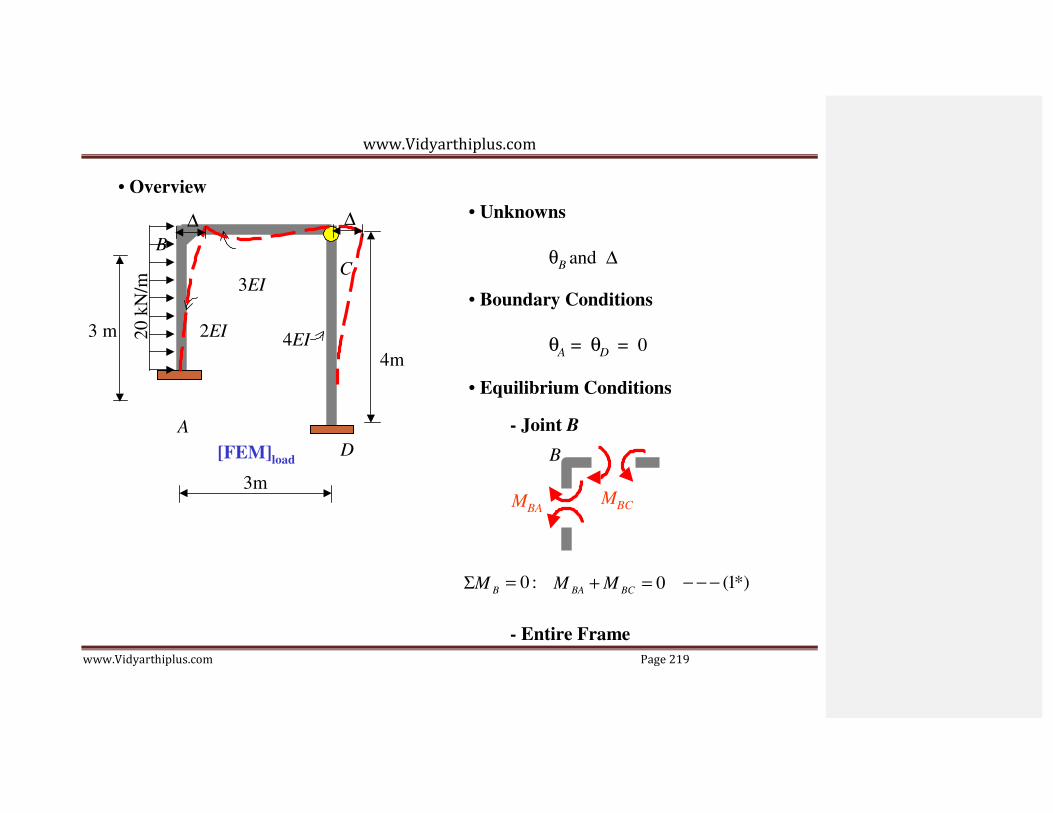
www.Vidyarthiplus.com
www.Vidyarthiplus.com Page 219
20 k
N/m
• Overview
∆ ∆ B
C 3EI
• Unknowns
θB and ∆
• Boundary Conditions
3 m 2EI
4EI
θ = θ
= 0
4m A D
A
[FEM]load D
3m
• Equilibrium Conditions
- Joint B
B
MBA MBC
ΣM B = 0 : M
BA + M
BC = 0 − − − (1*)
- Entire Frame

www.Vidyarthiplus.com
www.Vidyarthiplus.com Page 220
+
→ ΣFx
= 0 :
60 − Ax − Dx = 0
− − − (2*) 83

www.Vidyarthiplus.com
www.Vidyarthiplus.com Page 221
20 k
N/m
• Slope-Deflection Equation
3m
B
C
∆ ∆ B C
6(2EI∆)/(3) 2
3 m
3EI wL2/12 = 15
2EI
4EI
= 1.333EI∆ 1.5EI∆
wL2/12 = 15 4m
A
[FEM]load D
6(2EI∆)/(3) 2
= 1.333EI∆ 6(4EI∆)/(4) 2
A = 1.5EI∆ (1/2)(1.5EI∆)
M AB
M BA
= 4(2EI )
3
= 2(2EI )
3
0
θ A
+
0
θ A
+
2(2EI )
θ 3
B
4(2EI ) θ
3 B
+ 15 + 1.333EI∆
−15 + 1.333EI∆
= 1.333EIθ B
= 2.667 EIθ B
[FEM]∆
+ 15 + 1.333EI∆
− 15 + 1.333EI∆
D
----------(1)
----------(2)
M BC
= 3(3EI )
θ 3
B
0
= 3EIθ B

www.Vidyarthiplus.com
www.Vidyarthiplus.com Page 222
----------(3)
M DC =
3(4EI ) θ
4 D
+ 0.75EI∆
= 0.75EI∆
----------(4)
84

www.Vidyarthiplus.com
www.Vidyarthiplus.com Page 223
• Horizontal reactions
MAB
C
B
1.5 m
+ ΣM B
= 0 :
M + M
+ 60(1.5)
60 kN
4 m A
x = BA AB
3
1.5 m
A
Ax
= 1.333EIθ B
+ 0.889EI∆ + 30 − − − (5)
Ax D Dx
MDC
+ ΣMC = 0:
M MBA D = DC = 0.188EI∆
x 4
− − − (6)

www.Vidyarthiplus.com
www.Vidyarthiplus.com Page 224
85

www.Vidyarthiplus.com
www.Vidyarthiplus.com Page 225
Equilibrium Conditions • Solve equation
M BA
+ M BC
= 0
60 − Ax − Dx = 0 − − − (1*)
− − − (2*)
Substitute (2) and (3) in (1*)
5.667 EIθ B + 1.333EI∆ = 15 − − − (7)
Equation of moment Substitute (5) and (6) in (2*)
M AB
= 1.333EIθ B
+ 15 + 1.333EI∆
− − − (1) −1.333EIθ
B −1.077EI∆ = −30 − − − (8)
M BA
= 2.667 EIθ B
− 15 + 1.333EI∆
− − − (2)
From (7) and (8), solve equations;
M BC
= 3EIθ B
− − − (3)
θ B
= − 5.51
EI ∆ =
34.67 EI
M DC
= 0.75EI∆ − − − (4)
Substituteθ B
= − 5.51
and EI
∆ = 34.67
EI
in (1)to (6)
Horizontal reaction at support
M AB
M BA
= 53.87 kN • m
= 16.52 kN • m
Ax
= 1.333EIθ B
Dx = 0.188EI∆
+ 0.889EI∆ + 30
− − − (6)
− − − (5) M BC
M DC
= −16.52 kN • m
= 26.0 kN • m

www.Vidyarthiplus.com
www.Vidyarthiplus.com Page 226
Ax = 53.48 kN
Dx = 6.52 kN 86

www.Vidyarthiplus.com
www.Vidyarthiplus.com Page 227
B 3m
C
16.52 kN•m
3 m
53.87 kN•m 4m
M AB
M BA
M BC
M DC
= 53.87 kN • m
= 16.52 kN • m
= −16.52 kN • m
= 26.0 kN • m
53.48 kN
A 5.55 kN D
26 kN•m
6.52 kN
Ax = 53.48 kN
Dx = 6.52 kN
16.52
5.55 kN
16.52 ∆ ∆
B C B C
53.87

www.Vidyarthiplus.com
www.Vidyarthiplus.com Page 228
A

www.Vidyarthiplus.com
www.Vidyarthiplus.com Page 229
Example
The statically indeterminate beam shown in the figure is to be analysed.
• Members AB, BC, CD have the same length .
• Flexural rigidities are EI, 2EI, EI respectively.
• Concentrated load of magnitude acts at a distance from the
support A.
• Uniform load of intensity acts on BC.
• Member CD is loaded at its midspan with a concentrated load of magnitude
.
In the following calcuations, clockwise moments and rotations are positive.
Degrees of freedom
Rotation angles θA, θB, θC, θD of joints A, B, C, D respectively are taken as the unknowns. There
are no chord rotations due to other causes including support settlement.
Fixed end moments
Fixed end moments are:

www.Vidyarthiplus.com
www.Vidyarthiplus.com Page 230
Slope deflection equations
The slope deflection equations are constructed as follows:
Joint equilibrium equations
Joints A, B, C should suffice the equilibrium condition. Therefore
Rotation angles
The rotation angles are calculated from simultaneous equations above.
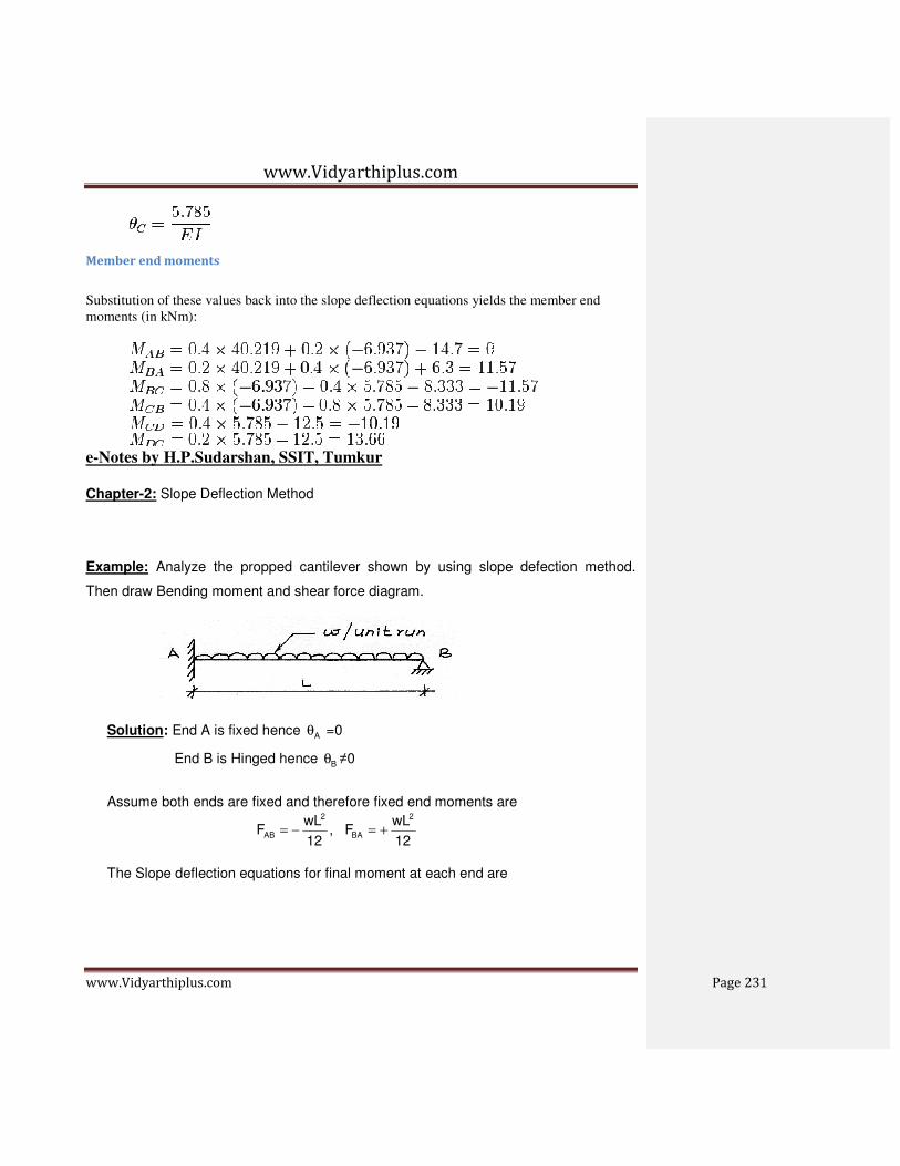
www.Vidyarthiplus.com
www.Vidyarthiplus.com Page 231
Member end moments
Substitution of these values back into the slope deflection equations yields the member end
moments (in kNm):
e-Notes by H.P.Sudarshan, SSIT, Tumkur Chapter-2: Slope Deflection Method
Example: Analyze the propped cantilever shown by using slope defection method.
Then draw Bending moment and shear force diagram.
Solution: End A is fixed hence Aθ =0
End B is Hinged hence Bθ ≠0
Assume both ends are fixed and therefore fixed end moments are
12
wLF,
12
wLF
2
BA
2
AB +=−=
The Slope deflection equations for final moment at each end are

www.Vidyarthiplus.com
www.Vidyarthiplus.com Page 232
( )
( )
)2(L
EI4
12
wL
2L
EI2FM
)1(L
EI2
12
wL
2L
EI2FM
B
2
ABBABA
B
2
BAABAB
→θ+=
θ+θ+=
→θ+−
=
θ+θ+=
In the above equations there is only one unknown Bθ .
To solve we have boundary condition at B;
Since B is simply supported, the BM at B is zero
ie. MBA=0.
iseanticlockw is rotation the indicates sign ve- 48
wLEI
0L
EI4
12
wLM(2) equation From
3
B
B
2
BA
−=θ∴
=θ+=∴
Substituting the value of BEIθ in equation (1) and (2) we have end moments
048
wL
L
4
12
wLM
iseanticlockw is moment indicates sign ve-8
wL
48
wL
L
2
12
wLM
32
BA
232
AB
=
−++=
−=
−+−=
MBA has to be zero, because it is hinged.
Now consider the free body diagram of the beam and find reactions using
equations of equilibrium.

www.Vidyarthiplus.com
www.Vidyarthiplus.com Page 233
wL8
3
wL8
5wLRwLR
wLRR
0V
wL8
5R
wL8
5
2
LwL
8
wL
2
LwLMLR
0M
AB
BA
A
2
ABA
B
=
−=−=
=+
=∑
=∴
+=×+=
×+=×
=∑
Problem can be treated as
The bending moment diagram for the given problem is as below

www.Vidyarthiplus.com
www.Vidyarthiplus.com Page 234
The max BM occurs where SF=0. Consider SF equation at a distance of x from
right support
2
2
Xmax
X
wL128
9
L8
3
2
wL
8
3wL
8
3MM
B support from L8
3 at occurs BMmax the Hence
L8
3X
0wXwL8
3S
=
−×==∴
=∴
=+−=
And point of contra flexure occurs where BM=0, Consider BM equation at a
distance of x from right support.
L4
3X
02
XwwLX
8
3M
2
X
=∴
=−=
For shear force diagram, consider SF equation from B

www.Vidyarthiplus.com
www.Vidyarthiplus.com Page 235
wL8
5SLS
wL8
3S0S
wXwL8
3S
AX
BX
X
+===
+===
−+=
Example: Analyze two span continuous beam ABC by slope deflection method. Then
draw Bending moment & Shear force diagram. Take EI constant
Solution: Fixed end moments are:
KNM67.4112
520
12
wLF
KNM67.4112
520
12
wLF
KNM89.886
24100
L
bWaF
KNM44.446
24100
L
WabF
22
CB
22
BC
2
2
2
2
BA
2
2
2
2
AB
=×
=+
=
−=×
−=−
=
+=××
+=+=
−=××
−=−
=
Since A is fixed 0A =θ , ,0,0 CB ≠θ≠θ
Slope deflection equations are:

www.Vidyarthiplus.com
www.Vidyarthiplus.com Page 236
( )
( )
)2(EI3
289.88
6
2EI289.88
2L
EI2FM
)1(EI3
144.44
6
EI244.44
2L
EI2FM
B
B
ABBABA
B
B
BAABAB
→−−−−θ+=
θ×++=
θ+θ+=
→−−−−θ+−=
θ+−=
θ+θ+=
( )
( )
( )
( )
)4(EI5
2
5
EI467.41
25
EI267.41
2L
EI2FM
)3(EI5
2EI
5
467.41
25
EI267.41
2L
EI2FM
BC
BC
BCCBCB
CB
CB
CBBCBC
→−−−−θ+θ+=
θ+θ++=
θ+θ+=
→−−−−θ+θ+−=
θ+θ+−=
θ+θ+=
In all the above four equations there are only two unknown Bθ and Cθ . And
accordingly the boundary conditions are
i -MBA-MBC=0
MBA+MBC=0
ii MCB=0 since C is end simply support.

www.Vidyarthiplus.com
www.Vidyarthiplus.com Page 237
)6(0EI5
4EI
5
267.41M
)5(0EI5
2EI
15
2222.47
EI5
2EI
5
467.41EI
3
289.88MMNow
CBCB
CB
CBBBCBA
>−−−−−=θ+θ+=
>−−−−−=θ+θ+=
θ+θ+−θ+=+
Solving simultaneous equations 5 & 6 we get
EI Bθ = – 20.83 Rotation anticlockwise.
EI Cθ = – 41.67 Rotation anticlockwise.
Substituting in the slope definition equations
MAB = – 44.44 + ( ) KNM38.5183.203
1−=−
MBA = + 88.89 + ( ) KNM00.7583.203
2+=−
MBC = – 41.67+ ( ) ( ) KNM00.7567.415
283.20
5
4−=−+−
MCB = + 41.67+ ( ) ( ) 067.415
483.20
5
2=−+−
Reactions: Consider the free body diagram of the beam.

www.Vidyarthiplus.com
www.Vidyarthiplus.com Page 238
Find reactions using equations of equilibrium.
Span AB: ΣMA = 0 RB×6 = 100×4+75-51.38
∴RB = 70.60 KN
ΣV = 0 RA+RB = 100KN
∴RA = 100-70.60=29.40 KN
Span BC: ΣMC = 0 RB×5 = 20×5×2
5+75
∴RB = 65 KN
ΣV=0 RB+RC = 20×5 = 100KN
RC = 100-65 = 35 KN
Using these data BM and SF diagram can be drawn.

www.Vidyarthiplus.com
www.Vidyarthiplus.com Page 239
Max BM:
Span AB: Max BM in span AB occurs under point load and can be found
geometrically
Mmax=113.33-51.38 -( )
KNM20.4646
38.5175=×
−
Span BC:Max BM in span BC occurs where shear force is zero or changes its
sign. Hence consider SF equation w.r.t C
Sx = 35-20x = 0 20
35x =∴ =1.75m
Max BM occurs at 1.75m from C
∴Mmax = 35 × 1.75 – 20 2
75.1 2
× = 30.625 KNM

www.Vidyarthiplus.com
www.Vidyarthiplus.com Page 240
Example: Analyze continuous beam ABCD by slope deflection method and then draw bending moment diagram. Take EI constant.
Solution:
0 ,0 ,0 CBA =θ=θ=θ
FEMS M KN 44.44 - 6
24100
L
Wab F
2
2
2
2
AB =××
−=−=
KNM 88.88 6
24100
L
bWa F
2
2
2
2
BA +=××
+=+=
KNM 41.67- 12
520
12
wLF
22
BC=
×−=−=
KNM 41.67 12
520
12
wLF
22
CB+=
×+=+=
M KN 30 - 5.120FCD =×−=
Slope deflection equations:
( ) ( )1--------- EI3
144.442
L
EI2FM BBAABAB >θ+−=θ+θ+=
( ) ( )2--------- EI3
289.882
L
EI2FM BABBABA >θ++=θ+θ+=
( ) ( )3-------- EI5
2EI
5
467.412
L
EI2FM CBCBBCBC >θ+θ+−=θ+θ+=
( ) ( )4-------- EI5
2EI
5
467.412
L
EI2FM BCBCCBCB >θ+θ++=θ+θ+=
KNM 30MCD −=
In the above equations we have two unknown rotations CB and θθ , accordingly the
boundary conditions are:

www.Vidyarthiplus.com
www.Vidyarthiplus.com Page 241
0MM
0MM
CDCB
BCBA
=+
=+
( )5-------- 0EI5
2EI
15
2222.47
EI5
2EI
5
467.41EI
3
289.88MM,Now
CB
CBBBCBA
>=θ+θ+=
θ+θ+−θ+=+
( )6EI5
4EI
5
267.11
30EI5
2EI
5
467.41MM,And
CB
BCCDCB
>−−−−−−θ+θ+=
−θ+θ++=+
Solving (5) and (6) we get
clockwise B @ Rotation 75.1EI
iseanticlockw B @ Rotation 67.32EI
C
B
+=θ
−=θ
Substituting value of BEIθ and CEIθ in slope deflection equations we have
( )
( )
( ) ( )
( ) ( )
KNM 30M
KNM 00.3067.325
275.1
5
467.41M
KNM 11.6775.15
267.32
5
467.41M
KNM 11.6767.323
289.88M
KNM 00.6167.322
144.44M
CD
CB
BC
BA
AB
−=
+=−+++=
−=+=−+−=
+=−++=
−=−+−=
Reactions: Consider free body diagram of beam AB, BC and CD as shown

www.Vidyarthiplus.com
www.Vidyarthiplus.com Page 242
ABSpan
KN 31.32R100R
KN 69.67R
6111.6741006R
BA
B
B
=−=
=
−+×=×
BC Span
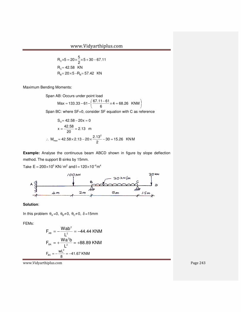
www.Vidyarthiplus.com
www.Vidyarthiplus.com Page 243
KN 42.57R520R
KN 58.42R
11.673052
5205R
BB
C
C
=−×=
=
−+××=×
Maximum Bending Moments:
Span AB: Occurs under point load
=×
−−−= KNM 26.684
6
6111.676133.133Max
Span BC: where SF=0, consider SF equation with C as reference
m 13.220
58.42x
0x2058.42SX
==
=−=
M KN 26.15302
13.22013.258.42M
2
max =−×−×=∴
Example: Analyse the continuous beam ABCD shown in figure by slope deflection
method. The support B sinks by 15mm.
Take 4625 m10120Iandm/KN10200E −×=×=
Solution:
In this problem Aθ =0, ≠θB 0, ≠θC 0, δ =15mm
FEMs:
KNM44.44L
WabF
2
2
AB−=−=
KNM89.88L
bWaF
2
2
BA+=+=
KNM67.418
wLF
2
BC −=−=

www.Vidyarthiplus.com
www.Vidyarthiplus.com Page 244
KNM67.418
wLF
2
CB +=+=
FEM due to yield of support B
For span AB:
KNM61000
151012010
6
2006
L
EI6mm
65
2
2baab
−=×××××
−=
δ−==
−
For span BC:
KNM64.81000
151012010
5
2006
L
EI6mm
65
2
2cbbc
+=×××××
+=
δ+==
−
Slope deflection equation

www.Vidyarthiplus.com
www.Vidyarthiplus.com Page 245
( )
( )
( )
( )
( )
( )
( )
( )5--------- KNM 30M
4--------- EI 5
2EI
5
431.50
64.82EI5
241.67
L
EI6)2(
L
EI2FM
3--------- EI 5
2EI
5
403.33
64.82EI5
241.67-
L
EI6)2(
L
EI2FM
2--------- EI3
289.82
6EI3
288.89
L
EI6)2(
L
EI2FM
1--------- EI3
144.50
6EI3
144.44-
L
EI62
L
EIF
)L
32(
L
EI2FM
CD
BC
BC
2BCCBCB
CB
CB
2CBBCBC
B
B
2ABBABA
B
B
2BAAB
BAABAB
>−=
>θ+θ++=
+θ+θ++=
δ+θ+θ+=
>θ+θ+−=
+θ+θ+=
δ+θ+θ+=
>θ++=
−θ++=
δ−θ+θ+=
>θ+−=
−θ+=
δ−θ+θ+=
δ−θ+θ+=
There are only two unknown rotations Bθ and Cθ . Accordingly the boundary conditions
are
Now,
0EI5
4EI
5
231.20MM
0EI5
2EI
15
2286.49MM
0MM
0MM
CBCDCB
CBBCBA
CDCB
BCBA
=θ+θ+=+
=θ+θ+=+
=+
=+
Solving these equations we get

www.Vidyarthiplus.com
www.Vidyarthiplus.com Page 246
ockwise Anticl71.9EI
ockwise Anticl35.31EI
C
B
−=θ
−=θ
Substituting these values in slope deflections we get the final moments:
( )
( )
( ) ( )
( ) ( )
KNM 30M
KNM 00.3035.315
271.9
5
431.50M
KNM 99.6171.95
235.31
5
403.33M
KNM 99.6135.313
289.82M
KNM 89.6035.313
144.50M
CD
CB
BC
BA
AB
−=
+=−+−++=
−=−+−+−=
+=−++=
−=−+−=
Consider the free body diagram of continuous beam for finding reactions
Reactions: Span AB: RB × 6 = 100 x 4 + 61.99 – 60.89
RB = 66.85
RA = 100 – RB
=33.15 KN
Span BC:
RB × 5 = 20 x 5 x 2
5+ 61.99 – 30
RB = 56.40 KN
RC = 20 x 5 - RB
=43.60 KN

www.Vidyarthiplus.com
www.Vidyarthiplus.com Page 247
Example: Three span continuous beam ABCD is fixed at A and continuous over B, C
and D. The beam subjected to loads as shown. Analyse the beam by slope deflection
method and draw bending moment and shear force diagram.
Solution:
Since end A is fixed 0,0,0,0 DcBA =θ≠θ≠θ=θ
FEMs:
KNM 30 - 8
460
8
Wl FAB =
×−=−=

www.Vidyarthiplus.com
www.Vidyarthiplus.com Page 248
KNM 30 8
460
8
Wl FBA +=
×+=+=
KNM 12.5 4
M FBC +=+=
KNM 12.5 4
M FCB +=+=
KNM 3 13.3 - 12
410
12
wl F
22
CD =×
−=−=
KNM 13.33 12
410
12
wl F
22
DC +=×
+=+=
Slope deflection equations:
( )BAABAB 2L
EI2F M θ+θ+=
( ) 04
EI2 30- Bθ++=
( ) 1-------- EI0.5 30- B >θ+=
( )ABBABA 2L
EI2F M θ+θ+=
( ) 024
EI2 30 B +θ+=
( ) 2--------- EI 30 B >θ++=
( )CBBCBC 2L
EI2F M θ+θ+=
( ) 24
EI2 12.5 CB θ+θ+=
( ) 3--------- EI5.0EI 12.5 CB >θ+θ+=
( )BCCBCB 2L
EI2F M θ+θ+=
( ) 24
EI2 5.12 BC θ+θ+=
( ) 4--------- EI 5.0EI 12.5 BC >θ+θ+=
( )DCCDCD 2L
EI2F M θ+θ+=
( ) 24
EI2 13.33- DC θ+θ+=
( ) 5---------- EI5.0 EI33.13 DC >θ+θ+−=
( )CDDCDC 2L
EI2F M θ+θ+=

www.Vidyarthiplus.com
www.Vidyarthiplus.com Page 249
( ) 24
EI2 13.33 CD θ+θ+=
( ) 6---------- EI EI5.013.33 DC >θ+θ+=
In the above Equations there are three unknowns, EI DCB EI&EI, θθθ , accordingly the
boundary conditions are:
)hinged(0Miii
0MMii
0MMi
DC
CDCB
BCBA
Q=
=+
=+
Now
( )705.42EI5.0EI2
0EI5.0EI5.12EI30
0MM
CB
CBB
BCBA
>−−−−−−=+θ+θ
=θ+θ++θ+
=+
( )8083.0EI5.0EI2EI5.0
0EI5.0EI33.13EI5.0EI5.12
0MM
DCB
DCBC
BCCB
>−−−−−−=−θ+θ+θ
=θ+θ+−θ+θ++
=+
0MDC =
( )90EIEI5.033.13 DC >−−−−−−=θ+θ+
By solving (7), (8) & (9), we get
90.18EI
15.11EI
04.24EI
D
C
B
−=θ
+=θ
−=θ
By substituting the values of DcB and, θθθ in respective equations we get
( )( )
( ) ( )( )
( )( ) ( ) KNM 090.1815.115.033.13M
KNM 63.1190.185.015.1133.13M
KNM 63.1104.245.015.115.12M
KNM 5.96- 11.15.5024.04-12.5 M
KNM96.504.2430M
KNM 02.4204.245.030M
DC
CD
CB
BC
BA
AB
=−+++=
−=−++−=
+=−+++=
=++++=
+=−++=
−=−+−=
Reactions: Consider the free body diagram of beam.

www.Vidyarthiplus.com
www.Vidyarthiplus.com Page 250
Beam AB:
KN015.30R60R
KN985.204
02.4296.5260R
BA
B
=−=∴
=−+×
=
Beam BC:
downwardisRKN92.13RR
KN92.134
96.55063.11R
BCB
C
∴−=−=∴
=−+
=
Beam CD:
KN91.22R410R
KN09.174
63.112410R
DC
D
=−×=∴
=−××
=

www.Vidyarthiplus.com
www.Vidyarthiplus.com Page 251
Example: Analyse the continuous beam shown using slope deflection method. Then
draw bending moment and shear force diagram.
Solution: In this problem fixed isA end ,0 A Q=θ
FEMs:
MKN 53.33 - 12
810
12
wl F
22
AB =×
−=−=
KNM 53.33 12
wl F
2
BA +=+=
KNM 22.50 - 8
630
8
Wl FBC =
×−=−=
KNM 22.50 8
WL FCD +=+=
Slope deflection equations:
( )BAABAB 2L
EI2F M θ+θ+=
( ) 08
I3E2 53.33- Bθ+
×+=
( ) 1-------- EI 4
3 53.33- B >θ+=
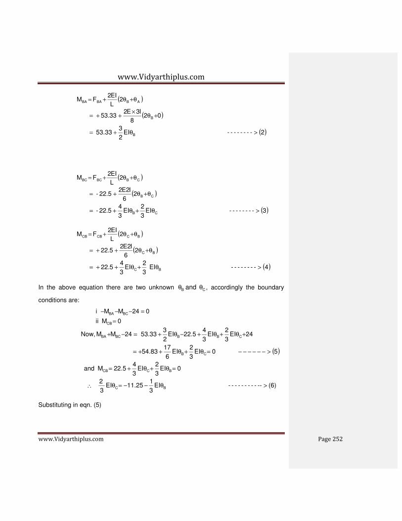
www.Vidyarthiplus.com
www.Vidyarthiplus.com Page 252
( )ABBABA 2L
EI2F M θ+θ+=
( ) 028
I3E2 53.33 B +θ
×++=
( ) 2-------- EI2
3 53.33 B >θ+=
( )CBBCBC 2L
EI2F M θ+θ+=
( ) 26
I2E2 22.5- CB θ+θ+=
( ) 3-------- EI3
2EI
3
4 22.5- CB >θ+θ+=
( )BCCBCB 2L
EI2F M θ+θ+=
( ) 26
I2E2 22.5 BC θ+θ++=
( ) 4-------- EI 3
2EI
3
422.5 BC >θ+θ++=
In the above equation there are two unknown C B and θθ , accordingly the boundary
conditions are:
0Mii
024MMi
CB
BCBA
=
=−−−
( )50EI3
2EI
6
1783.54
24EI3
2EI
3
45.22EI
2
333.5324MM,Now
CB
CBBBCBA
>−−−−−−=θ+θ++=
+θ+θ+−θ+=−+
0EI3
2EI
3
45.22Mand BCCB =θ+θ+=
∴ (6)----------- EI3
125.11EI
3
2BC >θ−−=θ
Substituting in eqn. (5)

www.Vidyarthiplus.com
www.Vidyarthiplus.com Page 253
clockwiseanti rotation 432.1715
658.44EI
0EI6
1544.58
0EI3
125.11EI
6
1783.54
B
B
BB
−=×
−=θ∴
=θ++
=θ−−θ+
∴ from equation (6)
( )
iseanticlockw rotation 159.8
432.173
125.11
2
3EI C
−=
−−−=θ
Substituting 159.8EI and 432.17EI CB −=θ−=θ in the slope deflection equation we get
Final Moments:
( )
( ) KNM 18.27432.172
333.53M
KNM -66.40 17.432- 4
333.53M
BA
AB
+=−++=
=+−=
( ) ( )
( ) 00.0)432.17(3
2159.8
3
45.22M
KNM 18.51159.83
2432.17
3
45.22M
CB
BC
=−+−++=
−=−+−+−=
Reactions: Consider free body diagram of beams as shown
Span AB:
KN 87.44R810R
KN 13.358
481040.6618.27R
BA
B
=−×=∴
=××+−
=

www.Vidyarthiplus.com
www.Vidyarthiplus.com Page 254
Span BC:
KN 47.6R30R
KN 53.236
33018.51R
BC
B
=−=
=×+
=
Max BM Span AB: Max BM occurs where SF=0, consider SF equation with A as origin
KNM 67.36642
487.410487.487.44M
m 487.4x
010x-87.44S
2
max
x
=−×−×=∴
=
==
Span BC: Max BM occurs under point load

www.Vidyarthiplus.com
www.Vidyarthiplus.com Page 255
M KN 41.192
18.5145M BC max =−=
Example: Analyse the beam shown in figure. End support C is subjected to an
anticlockwise moment of 12 KNM.
Solution: In this problem fixed is end ,0 A ∴=θ
FEMs:
KNM 67.2612
420
12
wl F
22
BC −=×
−=−=
KNM 26.67 12
wl F
2
CB +=+=
Slope deflection equations:
( )BAABAB 2L
EI2F M θ+θ+=
( ) 04
I2E2 0 Bθ++=
( ) 1--------- EI B >θ=
( )ABBABA 2L
EI2F M θ+θ+=
( ) 024
I2E2 0 B +θ+=
( ) 2--------- EI2 B >θ=
( )CBBCBC 2L
EI2F M θ+θ+=
( ) 24
I5.1E2 26.67- CB θ+θ
×+=
( ) 3--------- EI4
3EI
2
3 26.67- CB >θ+θ+=
( )BCCBCB 2L
EI2F M θ+θ+=

www.Vidyarthiplus.com
www.Vidyarthiplus.com Page 256
( ) 24
I5.1E2 26.67 BC θ+θ
×++=
( ) 4--------- EI 4
3EI
2
326.67 BC >θ+θ++=
In the above equation there are two unknowns CB and θθ , accordingly the boundary
conditions are
012M
0MM
CB
BCBA
=+
=+
(5)--------- 067.26EI4
3EI
2
7
EI4
3EI
2
367.26EI2MM,Now
CB
CBBBCBA
>=−θ+θ=
θ+θ+−θ=+
(6)--------- 0EI2
3EI
4
367.38
12EI4
3EI
2
367.2612M,and
CB
BCCB
>=θ+θ+=
+θ+θ+=+
From (5) and (6)
72.1425
846EI
046EI8
25
033.19EI4
3EI
8
3
067.26EI4
3EI
2
7
B
B
CB
CB
+=×+=θ
=−θ
=+θ+θ
=−θ+θ
From (6)
( )
iseanticlockw rotation indicates sign ve- 14.33
72.144
367.38
3
2EI C
−=
+−=θ
equationsdeflectionslope isEI and EI ngSubstituti CB θθ
( )
KNM 12)72.14(4
3)14.33(
2
367.26M
KNM 44.2914.334
3)72.14(
2
367.26M
KNM 42.29)72.14(2EI2M
KNM 72.14EIM
CB
BC
BBA
BAB
−=+−++=
=−++−=
==θ=
+=θ=

www.Vidyarthiplus.com
www.Vidyarthiplus.com Page 257
Reaction: Consider free body diagrams of beam
Span AB:
KN04.11RR
KN 04.114
44.2972.14R
BA
B
−=−=
=+
=
Span BC:
KN 64.29R420R
KN36.504
24201244.29R
BC
B
=−×=
=××++
=

www.Vidyarthiplus.com
www.Vidyarthiplus.com Page 258
Example: Analyse the simple frame shown in figure. End A is fixed and ends B & C are hinged. Draw the bending moment diagram.
Solution:

www.Vidyarthiplus.com
www.Vidyarthiplus.com Page 259
In this problem ,0,0,0,0 DCBA ≠θ≠θ≠θ=θ
FEMS:-
KNM108
WLF
KNM108
420
8
WLF
KNM67.2612
420
12
wlF
KNM67.2612
420
12
wlF
KNM33.536
42120
L
bWaF
KNM67.1066
42120
L
WabF
DB
CD
22
CB
22
BC
2
2
2
2
BA
2
2
2
2
AB
−=−=
+=×
+=+=
+=×
+=+=
−=×
−=−=
+=××
+=+=
−=××
−=−=
Slope deflections are
( )
( ) )1(EI3
267.106
6
I2E267.106
2L
EI2FM
BB
BAABAB
>−−−−θ+−=θ+−=
θ+θ+=
( )
( )
( )
( )
( )
( ) )4(EI4
3EI
2
367.262
2
I3
4
E267.26
2L
EI2FM
)3(EI4
3EI
2
367.262
2
I3
4
E267.26
2L
EI2FM
)2(EI3
433.532
6
I2E233.53
2L
EI2FM
BCBC
BCCBCB
CBCB
CBCBBC
BB
BBBABA
>−−−−θ+θ++=θ+θ×++=
θ+θ+=
>−−−−θ+θ+−=θ+θ×+−=
θ+θ+=
>−−−−θ++=θ++=
θ+θ+=

www.Vidyarthiplus.com
www.Vidyarthiplus.com Page 260
( )
( )
( )
( ) )6(EI2
1EI102
4
EI210
2L
EI2FM
)5(EI2
1EI102
4
EI210
2L
EI2FM
BDBD
BDDBDB
DBDB
DBBDBD
>−−−−θ+θ+−=θ+θ+−=
θ+θ+=
>−−−−θ+θ++=θ+θ++=
θ+θ+=
In the above equations we have three unknown rotations Bθ , Cθ , Dθ accordingly we have
three boundary conditions.
0MMM BDBCBA =++
0MCB = Since C and D are hinged
0MDB =
Now
(9)----- 0EIEI2
110M
(8)----- 0EI2
3EI
4
36.672M
(7)----- 0EI2
1EI
4
3EI
6
2336.66
EI2
1EI10EI
4
3EI
2
367.26EI
3
433.53MMM
DBDB
CBCB
DCB
DBCBBBDBCBA
>=θ+θ+−=
>=θ+θ+=
>=θ+θ+θ+=
θ+θ++θ+θ+−θ+=++
Solving equations 7, 8, & 9 we get
414.14EI
36.13EI
83.8EI
D
C
B
+=θ
−=θ
−=θ
Substituting these values in slope equations
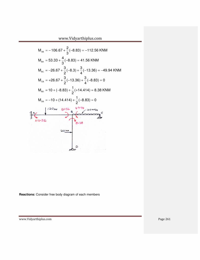
www.Vidyarthiplus.com
www.Vidyarthiplus.com Page 261
0)83.8(2
1)414.14(10M
KNM38.8)414.14(2
1)83.8(10M
0)83.8(4
3)36.13(
2
367.26M
KNM94.49)36.13(4
3)3.8(
2
367.26M
KNM56.41)83.8(3
433.53M
KNM56.112)83.8(3
267.106M
DB
BD
CB
BC
BA
AB
=−++−=
=++−+=
=−+−++=
−=−+−+−=
=−+=
−=−+−=
Reactions: Consider free body diagram of each members
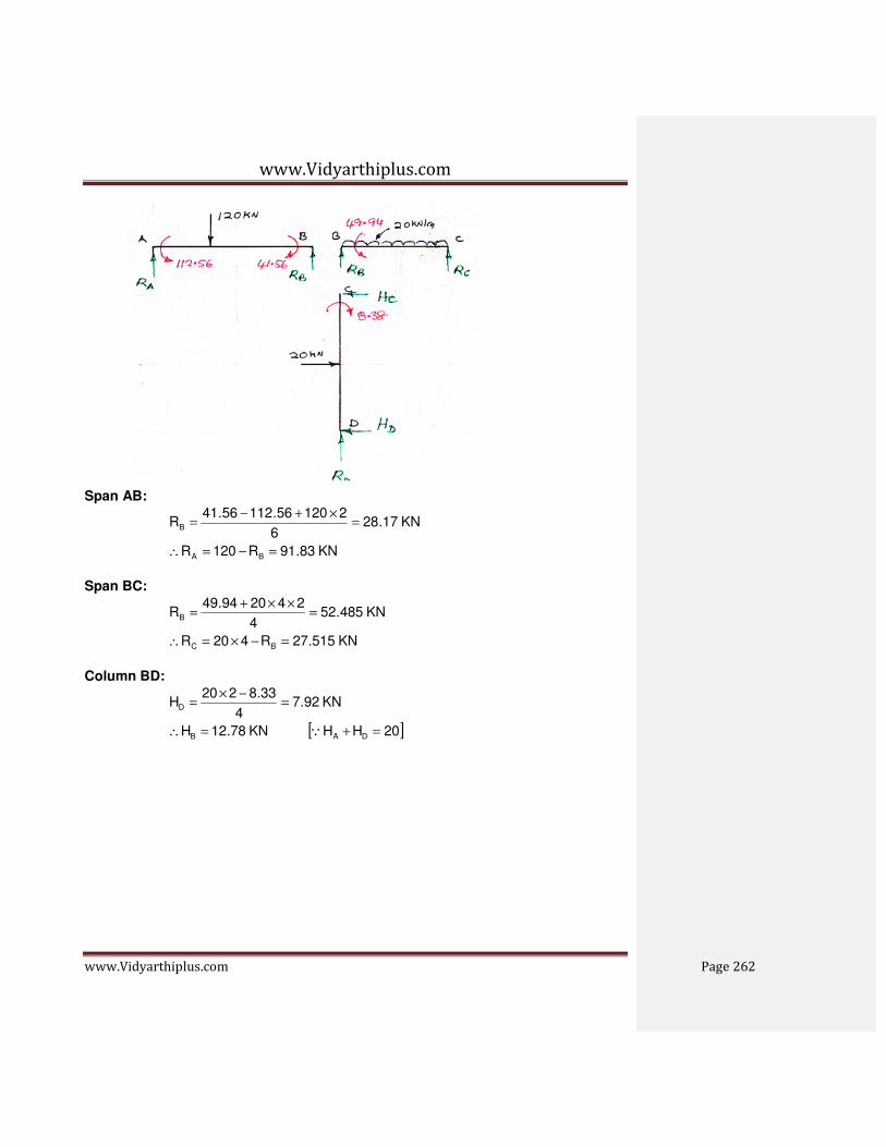
www.Vidyarthiplus.com
www.Vidyarthiplus.com Page 262
Span AB:
KN83.91R120R
KN17.286
212056.11256.41R
BA
B
=−=∴
=×+−
=
Span BC:
KN515.27R420R
KN485.524
242094.49R
BC
B
=−×=∴
=××+
=
Column BD:
[ ]20HHKN78.12H
KN92.74
33.8220H
DAB
D
=+=∴
=−×
=
Q

www.Vidyarthiplus.com
www.Vidyarthiplus.com Page 263
Example: Analyse the portal frame shown in figure and also drawn bending moment
and shear force diagram
Solution: Symmetrical problem - Sym frame + Sym loading
0 ,0 ,0 ,0 DCBA =θ≠θ≠θ=θ
FEMS
KNM 106.67 - 6
2480
6
4280
L
cdW
L
abWF
2
2
2
2
2
22
2
21
BC
=××
−××
=
−−=

www.Vidyarthiplus.com
www.Vidyarthiplus.com Page 264
KNM 67.106L
dcW
L
bWaF
2
22
2
2
CB +=++=
Slope deflection equations:
( ) ( ) ( )1-------- EI2
10
4
EI202
L
EI2FM BBBAABAB >θ=θ++=θ+θ+=
( ) ( ) ( )2------- EI024
EI202
L
EI2FM BBABBABA >θ=+θ+=θ+θ+=
( )
( )3------ EI3
2EI
3
467.106)2(
6
I2E267.106
2L
EI2FM
CBCB
CBBCBC
>θ+θ+−=θ+θ+−=
θ+θ+=
( )
( )4------ EI3
2EI
3
467.106)2(
6
I2E267.106
2L
EI2FM
BCBC
BCCBCB
>θ+θ++=θ+θ++=
θ+θ+=
( )
( )5------- EI)02(4
EI20
2L
EI2FM
CC
DCCDCD
>θ=+θ+=
θ+θ+=
( )
( )6------- EI2
1)0(
4
EI20
2L
EI2FM
CC
CDDCDC
>θ=θ++=
θ+θ+=
In the above equation there are two unknown rotations. Accordingly the boundary
conditions are
0MM
0MM
CDCB
BCBA
=+
=+
Now (7)------- 0EI3
2EI
3
767.106MM CBBCBA >=θ+θ+−=+
(8)------- 0EI3
7EI
3
267.106MM CBCDCB >=θ+θ++=+
Multiply by (7) and (8) by 2
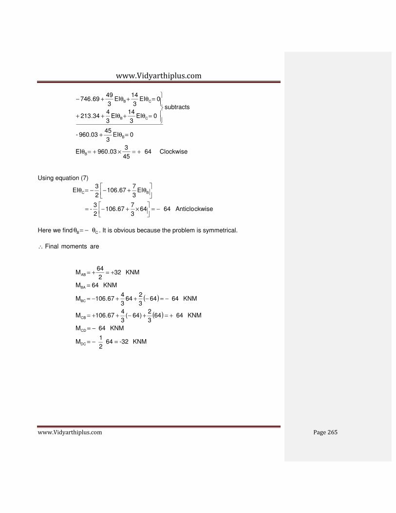
www.Vidyarthiplus.com
www.Vidyarthiplus.com Page 265
Clockwise 6445
3 03.960 EI
0EI3
45960.03-
subtracts
0EI3
14EI
3
434.213
0EI3
14EI
3
4969.746
B
B
CB
CB
+=×+=θ
=θ+
=θ+θ++
=θ+θ+−
Using equation (7)
ckwise Anticlo64643
767.106
2
3-
EI3
767.106
2
3EI BC
−=
×+−=
θ+−−=θ
Here we find CB θ−=θ . It is obvious because the problem is symmetrical.
are moments Final ∴
( )
( )
KNM -3264 2
1 M
KNM 64 M
KNM 64 643
2)64 (
3
467.106M
KNM 64 643
264
3
467.106M
KNM 64M
KNM 322
64M
DC
CD
CB
BC
BA
AB
=−=
−=
+=+−++=
−=−++−=
=
+=+=

www.Vidyarthiplus.com
www.Vidyarthiplus.com Page 266
Consider free body diagram’s of beam and columns as shown
By symmetrical we can write
KNM 80R R
KNM 60R R
CD
BA
==
==
Now consider free body diagram of column AB Apply
KN 24H
32644 H
0M
A
A
B
=∴
+=×
=∑

www.Vidyarthiplus.com
www.Vidyarthiplus.com Page 267
Similarly from free body diagram of column CD Apply
KN 24H
32644 H
0M
D
A
C
=∴
+=×
=∑
Check:
0HH
0H
DA =+
=∑
Hence okay

www.Vidyarthiplus.com
www.Vidyarthiplus.com Page 268
Note: Since symmetrical, only half frame may be analysed. Using first three equations
and taking CB θ−=θ
Example: Analyse the portal frame and then draw the bending moment diagram
Solution:
This is a symmetrical frame and unsymmetrically loaded, thus it is an
unsymmetrical problem and there is a sway
Assume sway to right.
Here 0,0,0,0 DBDA =θ≠θ=θ=θ
FEMS:
KNM 75.938
3580
L
bWaF
KNM 25.568
3580
L
WabF
2
2
2
2
CB
2
2
2
2
BC
+=××
+=+=
−=××
−=−=
Slope deflection equations

www.Vidyarthiplus.com
www.Vidyarthiplus.com Page 269
( )
( )2-------- EI8
3EI
4
302
4
2EI0
L
32
L
EI2FM
1-------- EI8
3EI
2
1
4
30
4
2EI0
L
32
L
EI2FM
BB
ABBABA
BB
BAABAB
>δ−θ=
δ−+θ+=
δ−θ+θ+=
>δ−θ=
δ−θ++=
δ−θ+θ+=
( )
( ) ( )
( )
( ) ( )
( )
( )6--------- EI8
3EI
2
1
4
30
4
2EI0
L
32
L
EI2FM
5--------- EI8
3EI
4
302
4
2EI0
L
32
L
EI2FM
4--------- EI4
1EI
2
175.932
8
2EI75.93
2L
EI2FM
3--------- EI4
1EI
2
125.562
8
2EI25.56
2L
EI2FM
CC
CDDCDC
CC
DCCDCD
BCBC
BCCBCB
CBCB
CBBCBC
>δ−θ=
δ−θ++=
δ−θ+θ+=
>δ−θ=
δ−+θ+=
δ−θ+θ+=
>θ+θ+=θ+θ++=
θ+θ+=
>θ+θ+−=θ+θ+−=
θ+θ+=
In the above equation there are three unknowns δθθ and, CB , accordingly the
boundary conditions are,
0MMMM
04
MM
4
MM,e.i
condition Shear - -- 0PHH
0MM
conditionsintJo0MM
DCCDBAAB
DCCDBAAB
HDA
CDCB
BCBA
=+++∴
=+
++
>=∑++
=+
>−−=+

www.Vidyarthiplus.com
www.Vidyarthiplus.com Page 270
( )70EI8
3EI
4
1EI
2
325.56
0EI4
1EI
2
125.56EI
8
3EIMM,Now
CB
CBBBCBA
>−−−−−−=δ−θ+θ+−=
=θ+θ+−δ−θ=+
( )80EI8
3EI
2
3EI
4
175.93
0EI8
3EIEI
4
1EI
2
175.93MM,And
CB
CBCCDCB
>−−−−−−−=δ−θ+θ+=
=δ−θ+θ+θ+=+
( )90EI2
3EI
2
3EI
2
3
EI`8
3EI
2
1
EI8
3EIEI
8
3EIEI
8
3EI
2
1MMMM,And
CB
C
CBBDCCDBAAB
>−−−−−−−=δ−θ+θ=
δ−θ+
δ−θ+δ−θ+δ−θ=+++
(8) & (7) in Substitute
EIEIEI (9) From CB θ+θ=δ
(7) Eqn
[ ]
( )10-------0EI8
1EI
8
925.56
0EIEI8
3EI
4
1EI
2
325.56
CB
CBCB
>−−=θ−θ+−
=θ+θ−θ+θ+−
)8(Eqn
[ ]
( ) 11----------0EI8
9EI
8
175.93
0EIEI8
3EI
2
3EI
4
175.93
CB
CBCB
>=θ+θ−+
=θ+θ−θ+θ++
Solving equations (10) & (11) we get 25.41EI B=θ
By Equation (10)
5.3775.7825.41EIEIEI
75.7825.418
925.568
EI8
925.568EI
CB
BC
−=−=θ+θ=δ∴
−=
+−=
θ+−=θ
Hence
5.37EI,75.78EI,25.41EI CB −=δ−=θ=θ
Substituting these values in slope deflection equations, we have

www.Vidyarthiplus.com
www.Vidyarthiplus.com Page 271
( ) ( )
( )
( ) ( )
( ) ( )
( )
( ) ( ) KNM31.255.378
375.78
2
1M
KNM69.645.378
375.78M
KNM69.6475.414
175.78
2
175.93M
KNM31.5575.784
125.41
2
125.56M
KNM31.555.378
325.41M
KNM69.345.378
325.41
2
1M
DC
CD
CB
BC
BA
AB
−=−−−=
−=−−−=
+=+−+=
−=−++−=
+=−−=
+=−−=
Reactions: consider the free body diagram of beam and columns Column AB:
KN5.224
31.5569.34HA =
+=
Span BC:
17.51R80R
KN83.288
38069.6431.55R
BC
B
=−=∴
=×+−
=
Column CD:
5.224
31.2569.64HD =
+=

www.Vidyarthiplus.com
www.Vidyarthiplus.com Page 272
Check: ΣH = 0
HA + HD = 0 22.5 – 22.5 = 0 Hence okay
Example: Frame ABCD is subjected to a horizontal force of 20 KN at joint C as shown in figure. Analyse and draw bending moment diagram.

www.Vidyarthiplus.com
www.Vidyarthiplus.com Page 273
Solution:
Frame is Symmetrical and unsymmetrical loaded hence there is a sway. Assume
sway towards right
FEMS
0FFFFFF DCCDCBBCBAAB ======
Slope deflection equations are
( )
( )2EI3
2EI
3
4
3
32
3
EI2
L
32
L
EI2FM
1--------- EI3
2EI
3
2
3
3
3
EI2
L
32
L
EI2FM
B
B
ABBABA
B
B
BAABAB
>−−−−−−δ−θ=
δ−θ=
δ−θ+θ+=
>δ−θ=
δ−θ=
δ−θ+θ+=
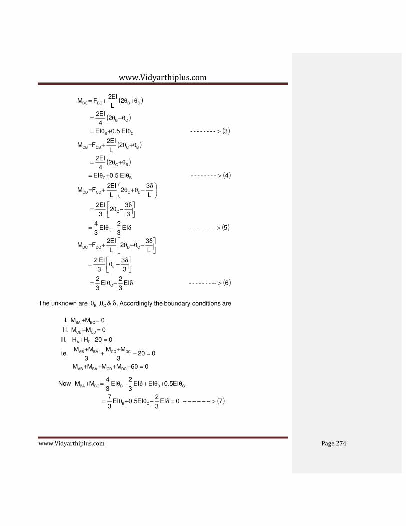
www.Vidyarthiplus.com
www.Vidyarthiplus.com Page 274
( )
( )
( )
( )
( )
( )
( )5EI3
2EI
3
4
3
32
3
2EI
L
32
L
EI2FM
4-------- EI5.0EI
24
EI2
2L
EI2FM
3-------- EI5.0EI
24
EI2
2L
EI2FM
C
C
DCCDCD
BC
BC
BCCBCB
CB
CB
CBBCBC
>−−−−−−δ−θ=
δ−θ=
δ−θ+θ+=
>θ+θ=
θ+θ=
θ+θ+=
>θ+θ=
θ+θ=
θ+θ+=
( )6--------- EI3
2EI
3
2
3
3
3
EI2
L
32
L
EI2FM
C
c
CDDCDC
>δ−θ=
δ−θ=
δ−θ+θ+=
The unknown are δθθ &, C,B . are conditionsboundary they Accordingl
060MMMM
0203
MM
3
MM,e.i
020HH.III
0MM.II
0MM.I
DCCDBAAB
DCCDBAAB
DA
CDCB
BCBA
=−+++
=−+
++
=−+
=+
=+
( )70EI3
2EI5.0EI
3
7
EI5.0EIEI3
2EI
3
4MMNow
CB
CBBBCBA
>−−−−−−=δ−θ+θ=
θ+θ+δ−θ=+

www.Vidyarthiplus.com
www.Vidyarthiplus.com Page 275
( )80EI3
2EI
3
7EI5.0
EI3
2EI
3
4EI5.0EIMMand
CB
CBCCDCB
>−−−−−−=δ−θ+θ=
δ−θ+θ+θ=+
( )9060EI3
8EI2EI2
60EI3
2EI
3
2EI
3
2
EI3
4EI
3
2EI
3
4EI
3
2EI
3
260MMMMand
CB
C
CBBDCCDBAAB
−−−−−−−=−δ−θ+θ=
−δ−θ+δ−
θ+δ−θ+δ−θ=−+++
Solving (7).(8) & (9) we get
77.34EI
,18.8EI
,18.8EI
C
B
−=δ
−=θ
−=θ
Substituting the value of δθθ and, CB in slope deflection equations
( ) ( )
( ) ( )
( )( )
( ) ( )
( ) ( ) KNM73.1777.343
218.8
3
2M
KNM27.1277.343
218.8
3
4M
KNM27.1218.818.85.0M
KNM27.1218.85.018.80M
KNM27.1277.343
218.8
3
4M
KNM73.1777.343
218.8
3
2M
DC
CD
CB
BC
BA
AB
+=−−−=
+=−−−=
−=−−=
−=−+−=
+=−−−=
+=−−−=

www.Vidyarthiplus.com
www.Vidyarthiplus.com Page 276
Reactions: Consider the free body diagram of the members
Member AB:
KN103
27.1273.17HA =
+=
Member BC:
downwardsR of direction indicates sign ve-KN135.6RR
KN135.64
27.1227.12R
BCB
C
−=−=∴
=+
=
Member CD:

www.Vidyarthiplus.com
www.Vidyarthiplus.com Page 277
righttoleftisH of direction the indicates sign ve- KN103
27.1273.17H DD −=
−−=
Check: ΣH = 0
HA + HD + P = 0
+10 + 10 – 20 = 0
Hence okay
Example: Analyse the portal frame subjected to loads as shown. Also draw bending
moment diagram.
The frame is symmetrical but loading is unsymmetrical. Hence there is a sway.
Assume sway towards right. In this problem 0 ,0 ,0 ,0 DCBA =θ≠θ≠θ=θ
FEMs:
KNM 13.33 - 12
410
12
wl F
22
AB =×
−=−=
KNM 13.33 12
410
12
wl F
22
BA +=×
+=+=

www.Vidyarthiplus.com
www.Vidyarthiplus.com Page 278
KNM 112.5 - 8
1090
8
wl FBC =
×−=−=
KNM 112.5 8
1090
8
wl FCB +=
×==
Slope deflection equations:
δ+θ+θ+=
L
32
L
EI2F M BAABAB
4
30
4
EI2 13.33- B
δ−θ++=
( ) 1--------- EI 375.0 EI 5.0 13.33- B >δ−θ+=
δ+θ+θ+=
L
32
L
EI2F M ABBABA
4
302
4
EI2 13.33 B
δ−+θ+=
( ) 2--------- EI 375.0EI 13.33 B >δ−θ+=
( )CBBCBC 2L
EI2F M θ+θ+=
( ) 210
I3E2 112.5- CB θ+θ+=
( ) 3--------- EI6.01.2EI 112.5- CB >θ+θ+=
( )BCCBCB 2L
EI2F M θ+θ+=
( ) 210
I3E2 112.5 BC θ+θ++=
( ) 4--------- EI 6.01.2EI 112.5 BC >θ+θ+=
δ−θ+θ+=
L
32
L
EI2F M DCCDCD
4
302
4
EI2 0 C
δ−+θ+=
( ) 5--------- EI 375.0 EI C >δ−θ=
δ−θ+θ+=
L
32
L
EI2F M CDDCDC
4
320
4
EI2 0 C
δ−θ++=
( ) 6--------- EI 375.0 0.5EI C >δ−θ=
δθθ EI andEIEI unknowns 3 are There C B, , accordingly the boundary conditions are

www.Vidyarthiplus.com
www.Vidyarthiplus.com Page 279
040HH
0MM
0MM
DA
CDCB
BCBA
=++
=+
=+
4
MMH
MM4Hand
4
80 M M H
2
4410 M M 4 HHere
DCCDD
BCCDD
BAABA
BAABA
+=
+=×
−+=
××−+=×
080MMM M
0404
MM
4
80 M M
DCCDBAAB
DCCDBAAB
=++++
=++
+−+
∴
Now MBA + MBC = 0
( ) ( )
(8)-------- 0EI375.0EI6.0 EI2.25.112
0EI375.0EIEI6.0EI2.15.112
5 4 0MMand
(7)-------- 017.99EI375.0EI6.0 EI2.2
0EI6.0EI2.15.112EI375.0EI33.13
BC
CBC
DCCB
CB
CBB
>=δ−θ+θ+
=δ−θ+θ+θ+
+=+
>=−δ−θ+θ
=θ+θ+−δ−θ
(9)---------080EI-1.5EI1.5EI5.1
080EI375.0EI5.0
EI375.0EIEI375.0EI33.13EI375.0EI5.033.13
080MMMM also
CB
C
CBB
DCCBBAAB
>=+δθ+θ
=+δ−θ+
δ−θ+θδ−θ++δ−θ+−
=++++
By solving (7), (8) and (9) we get
34.66EI
64.59EI
65.72EI
C
B
+=δ
−=θ
=θ
Final moments:
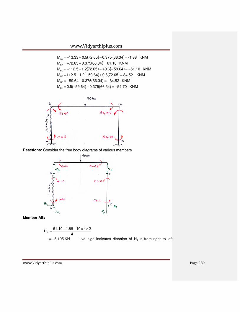
www.Vidyarthiplus.com
www.Vidyarthiplus.com Page 280
( ) ( )( )
( ) ( )( ) ( )
KNM 70.54)34.66(375.0)64.59(5.0M
KNM 52.84)34.66(375.064.59M
KNM 52.8465.726.064.592.15.112M
KNM 10.6164.596.065.722.15.112M
KNM 10.6134.66375.065.72M
KNM -1.88 66.34 375.065.725.033.13M
DC
CD
CB
BC
BA
AB
−=−−=
−=−−=
=+−+=
−=−+=+−=
=−+=
=−+−=
Reactions: Consider the free body diagrams of various members
Member AB:
left to right from isH of direction indicates sign ve-KN195.5
4
241088.110.61H
A
A
−=
××−−=

www.Vidyarthiplus.com
www.Vidyarthiplus.com Page 281
Member BC:
KN34.38R90R
KN34.4710
59010.6152.84R
CB
C
=−=∴
=×+−
=
Member CD
KN81.344
7.5454.84HD =
+=
Check
ΣH = 0
HA + HD +10 × 4 = 0
-5.20 - 34.81+ 40 = 0
Hence okay

www.Vidyarthiplus.com
www.Vidyarthiplus.com Page 282
Example: Analyse the portal frame and then draw the bending moment diagram
Solution:
Since the columns have different moment of inertia, it is an unsymmetrical frame.
Assume sway towards right
FEMS:
KNM 608
WLF
KNM 608
680
8
WLF
CB
BC
+=+=
−=×
−=−=
Here 0,0 DA =θ=θ
Slope deflection equations
( )
( )2-------- EI8
3EI
4
302
4
2EI0
L
32
L
EI2FM
1-------- EI8
3EI
2
1
4
30
4
2EI0
L
32
L
EI2FM
BB
ABBABA
BB
BAABAB
>δ−θ=
δ−+θ+=
δ−θ+θ+=
>δ−θ=
δ−θ++=
δ−θ+θ+=

www.Vidyarthiplus.com
www.Vidyarthiplus.com Page 283
( )
( ) ( )
( )
( ) ( )
( )
( )6--------- EI4
3EI
4
30
4
2E2I0
L
32
L
EI2FM
5--------- EI4
3EI2
4
302
4
2E2I0
L
32
L
EI2FM
4--------- EI3
4EI
3
2602
6
2E2I60
2L
EI2FM
3--------- EI3
2EI
3
4602
6
2E2I60
2L
EI2FM
CC
CDDCDC
CC
DCCDCD
CBBC
BCCBCB
CBCB
CBBCBC
>δ−θ=
δ−θ++=
δ−θ+θ+=
>δ−θ=
δ−+θ+=
δ−θ+θ+=
>θ+θ++=θ+θ+=
θ+θ+=
>θ+θ+−=θ+θ+−=
θ+θ+=
In the above equation there are three unknowns δθθ and, CB , accordingly the
boundary conditions are,
0MMMM
04
MM
4
MM,e.i
condition Shear - -- 0HH
conditionsintJo0MM
0MM
DCCDBAAB
DCCDBAAB
DA
CDCB
BCBA
=+++∴
=+
++
>=+
>−−=+
=+
( )70EI8
3EI
3
2EI
3
760
0EI3
2EI
3
460EI
8
3EIMM,Now
CB
CBBBCBA
>−−−−−−=δ−θ+θ+−=
=θ+θ+−δ−θ=+
( )8060EI4
3EI
3
10EI
3
2
0EI4
3EI2EI
3
4EI
3
260MM,And
CB
CCBCDCB
>−−−−−−−=+δ−θ+θ=
=δ−θ+θ+θ++=+

www.Vidyarthiplus.com
www.Vidyarthiplus.com Page 284
( )90EI4
9EI3EI
2
3
EI4
3EI
EI4
3EI2EI
8
3EIEI
8
3EI
2
1MMMM,And
CB
C
CBBDCCDBCAB
>−−−−−−−=δ−θ+θ=
δ−θ+
δ−θ+δ−θ+δ−θ=+++
(7) inEIofvaluengSubstituti
EI3EI2
3
9
4EI (9) From CB
δ
θ+θ=δ
( )10-------060EI6
1EI
12
25
060EI2
1EI
4
1EI
3
2EI
3
7
060EI3EI2
3
9
4
8
3EI
3
2EI
3
7
CB
CBCB
CBCB
>−−=−θ+θ
=−θ−θ−θ+θ
=−
θ+θ−θ+θ
Substituting value of EI δ in (8)
( )11-------060EI3
7EI
6
1
060EIEI2
1EI
3
10EI
3
2
060EI3EI2
3
9
4
8
3EI
3
10EI
3
2
CB
CBCB
CBCB
>−−=+θ+θ
=+θ−θ−θ+θ
=+
θ+θ−θ+θ
Solving (10) & (11) we get EI Bθ =31.03
By Equation (11)
3.27
60EI6
1
7
3EI BC
−=
+θ=θ
Now
55.16EI3EI2
3
9
4EI CB −=
θ+θ=δ
Now
EI Bθ =31.03, 3.27EI C −=θ , EI 55.16−=δ

www.Vidyarthiplus.com
www.Vidyarthiplus.com Page 285
Substituting these values in slope deflection equations, The final moments are:
( ) ( )
( )
( ) ( )
( ) ( )
( ) KNM52.1555.164
393.27M
KNM45.43)55.16(4
3)93.27(2M
KNM43.4393.273
403.31
3
260M
KNM25.3793.273
203.31
3
460M
KNM24.3755.168
303.31M
KNM72.2155.168
303.31
2
1M
DC
CD
CB
BC
BA
AB
−=−−−=
−=−−−=
+=−+++=
−=−++−=
=−−=
=−−=
Reactions: consider the free body diagram of beam and columns
Column AB:
KN74.144
72.2125.37HA =
+=

www.Vidyarthiplus.com
www.Vidyarthiplus.com Page 286
Beam BC:
03.41R80R
KN97.386
38045.4325.37R
BC
B
=−=∴
=×+−
=
Column CD:
KN74.144
52.1545.43HD =
+=
Check: ΣH = 0
HA + HD = 0 14.74-14.74=0 Hence okay
Ex: Portal frame shown is fixed at ends A and D, the joint B is rigid and joint C is hinged. Analyse the frame and draw BMD.

www.Vidyarthiplus.com
www.Vidyarthiplus.com Page 287
Solution: FEM’s:
0,0,0,0,0Here
KNM608
680
8
WLF
KNM608
680
8
WLF
CDCBBDA
CB
BC
≠θ≠θ≠θ=θ=θ
+=×
=+=
−=×−
=−=
Since C is hinged member CB and CD will rotate independently. Also the frame
is unsymmetrical, will also have sway. Let the sway be towards right.
The slope deflections are:
)1(EI8
3EI
2
1
4
30
4
EI20
L
32
L
EI2FM
B
B
BAABAB
>−−−−δ−θ=
δ−θ++=
δ−θ+θ+=

www.Vidyarthiplus.com
www.Vidyarthiplus.com Page 288
( )
( )
( )
)6(EI8
3EI
2
1
4
30
4
EI20
L
32
L
EI2FM
)5(EI8
3EI
4
302
4
EI20
L
32
L
EI2FM
)4(EI3
2EI
3
460
26
I2.E260
2L
EI2FM
)3(EI3
2EI
3
460
26
I2.E260
L
32
L
EI2FM
)2(EI8
3EI
4
302
4
EI20
L
32
L
EI2FM
CD
CD
CDDDCDC
CD
CD
DCDCDCD
BCB
BCB
BCBCBCB
CBB
CBB
CBBCBC
B
B
ABBABA
>−−−−δ−θ=
δ−θ++=
δ−θ+θ+=
>−−−−δ−θ=
δ−+θ+=
δ−θ+θ+=
>−−−−θ+θ++=
θ+θ++=
θ+θ+=
>−−−−θ+θ+−=
θ+θ+−=
δ−θ+θ+=
>−−−−δ−θ=
δ−+θ+=
δ−θ+θ+=
In the above equations areand,, CDCBB δθθθ unknowns. According the boundary
conditions are
I. MBA+MBC = 0,
II. MCB = 0,
III. MCD = 0,

www.Vidyarthiplus.com
www.Vidyarthiplus.com Page 289
IV. HA+HD = 0
0MMMM
04
MM
4
MM,e..i
DCCDBAAB
DCCDBAAB
=+++∴
=+
++
Now using the boundary conditions:
)14(060EI3
2EI
15
26
60EI3
2EI
5
3
3
7
060EI5
8
8
3EI
3
2EI
3
7MM
)7(EquationinngSubstituti
)13(EI5
8EI
2
3
15
16EIgives)12(Equation
)12(0EI16
15EI
2
3
0EI2
3EI
8
3
2
3EI
2
3MMMM
)10(inSub
)11(EI8
3EI)9(From
)10(0EI2
3EI
2
3EI
2
3
0EI8
3EI
2
1EI
8
3EIEI
8
3EIEI
8
3EI
2
1MMMM
)9(0EI8
3EIM
)8(060EI3
4EI
3
2M
)7(060EI8
3EI
3
2EI
3
7
EI3
2EI
3
460EI
8
3EIMM
CBB
CBB
BCBBBCBA
BB
B
BDCCDBAAB
cD
CDB
CDCDBBDCCDBAAB
CDCD
CBBCB
CBB
CBBBBCBA
>−−−−=−θ+θ=
−θ+θ
−=
=−
θ−θ+θ=+
>−−−−θ=θ×=δ
>−−−−=δ−θ=
=δ−
δ+θ=+++∴
>−−−−δ=θ
>−−−−=δ−θ+θ=
=δ−θ+δ−θ+δ−θ+δ−θ=+++
>−−−−=δ−θ=
>−−−−=+θ+θ=
>−−−−=−δ−θ+θ=
θ+θ+−δ−θ=+

www.Vidyarthiplus.com
www.Vidyarthiplus.com Page 290
have we2by (14) equation gmultiplyin and )8(EquationinngSubstituti
29.6442
15180EI
_____________________
0180EI15
42
_____________________
0120EI3
4EI
15
52
060EI3
4EI
3
2
B
B
CBB
CBB
=×=θ∴
=+θ−
=−θ+θ
=+θ+θ
864.10229.645
8EI
5
8EI From(13) B =×=θ=δ
574.38EI8
3EI (11) From CD =δ=θ
165.77
60864.1028
329.64
3
7
2
3
60EI8
3EI
3
7
2
3EI)7(From BCB
−=
−×−×−=
−δ−θ−=θ
864.102EI,57.38EI,165.77EI,29.64EI CDCBB =δ=θ−=θ=θ
∴Final Moments are
( ) ( )
( )
( ) ( )
( ) ( )
( )
( ) ( ) KNM29.19864.1028
3574.38
2
1M
0864.1028
3574.38M
029.643
2165.77
3
460M
KNM72.25165.773
229.64
3
460M
KNM72.25864.1028
329.64M
KNM42.6864.1028
329.64
2
1M
DC
CD
CB
BC
BA
AB
−=−=
=−=
=+−++=
−=−++−=
=−=
−=−=

www.Vidyarthiplus.com
www.Vidyarthiplus.com Page 291
Reactions: Consider the free body diagram of various members
Column AB:
KN825.44
42.672.25HA =
−=
Beam BC:
( )
KN71.3529.4480R
KN29.446
38072.25R
C
B
=−=
=×+
=
Column CD:
KN82.44
28.19HD ==
Check:
ΣH = 0
HA+HD = 0
Hence okay.

www.Vidyarthiplus.com
www.Vidyarthiplus.com Page 292
Example: Analyse the portal frame shown in figure the deflection method and then draw the bending moment diagram
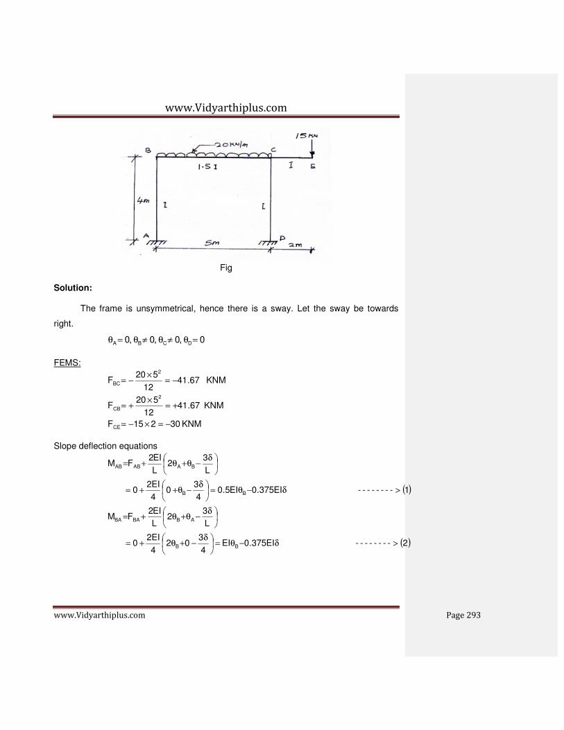
www.Vidyarthiplus.com
www.Vidyarthiplus.com Page 293
Fig
Solution:
The frame is unsymmetrical, hence there is a sway. Let the sway be towards
right.
0,0,0,0 DCBA =θ≠θ≠θ=θ
FEMS:
KNM 30215F
KNM 67.4112
520F
KNM 67.4112
520F
CE
2
CB
2
BC
−=×−=
+=×
+=
−=×
−=
Slope deflection equations
( )
( )2-------- EI375.0EI4
302
4
2EI0
L
32
L
EI2FM
1-------- EI375.0EI5.04
30
4
2EI0
L
32
L
EI2FM
BB
ABBABA
BB
BAABAB
>δ−θ=
δ−+θ+=
δ−θ+θ+=
>δ−θ=
δ−θ++=
δ−θ+θ+=

www.Vidyarthiplus.com
www.Vidyarthiplus.com Page 294
( )
( ) ( )
( )
( ) ( )
( )
( )6--------- EI375.0EI5.04
30
4
2EI0
L
32
L
EI2FM
5--------- EI375.0EI4
302
4
2EI0
L
32
L
EI2FM
4--------- EI6.0EI2.167.4125
1.5I2E67.41
2L
EI2FM
3--------- EI6.0EI2.167.4125
1.5I2E67.41
2L
EI2FM
CC
CDDCDC
CC
DCCDCD
BCBC
BCCBCB
CBCB
CBBCBC
>δ−θ=
δ−θ++=
δ−θ+θ+=
>δ−θ=
δ−+θ+=
δ−θ+θ+=
>θ+θ+=θ+θ×
++=
θ+θ+=
>θ+θ+−=θ+θ×
+−=
θ+θ+=
In the above equation there are three unknowns δθθ and, CB , accordingly the
boundary conditions are,
0MMMM,e.i
0HH
0MMM
0MM
DCCDBAAB
DA
CECDCB
BCBA
=+++
=+
=++
=+
Now,
( )7067.41EI375.0EI6.0EI2.2
0EI6.0EI2.167.141EI375.0EI
0MM
CB
CBB
BCBA
>−−−−−−=−δ−θ+θ=
=θ+θ+−δ−θ
=+
( )8067.11EI375.0EI2.2EI6.0
030EI375.0EIEI6.0EI2.167.41MM,And
CB
CBCCDCB
>−−−−−−−=+δ−θ+θ=
=−δ−θ+θ+θ+=+
( )90EI5.1EI5.1EI5.1
0EI375.0EI5.0EI375.0EI2EI375.0EIEI375.0EI5.0
0MMMM
CB
CCBB
DCCDBCAB
>−−−−−−−=δ−θ+θ
=δ−θ+δ−θ+δ−θ+δ−θ
=+++∴
Solving the above equations
we get, EI 98.23B =θ , EI 62.14EI,36.9C =δ−=θ

www.Vidyarthiplus.com
www.Vidyarthiplus.com Page 295
Substituting these values in slope deflection equations, we have
( ) ( )( )
( ) ( )( ) ( )
KNM30M
KNM16.1062.14375.036.95.0M
KNM84.14)62.14(375.036.9M
KNM83.4498.236.036.92.167.41M
KNM51.1836.96.098.232.167.41M
KNM50.1862.14375.098.23M
KNM50.662.14375.098.235.0M
CE
DC
CD
CB
BC
BA
AB
−=
−=×−−×=
−=+−−=
+=+−++=
−=−++−=
+=−=
=−=
Reactions: consider the free body diagram of beam and columns

www.Vidyarthiplus.com
www.Vidyarthiplus.com Page 296
Column AB:
KN25.64
5.65.18HA =
+=
Span BC:
73.44R520R
KN27.555
5.25205.1883.44R
CB
C
=−×=∴
=××+−
=
Column CD:
25.64
84.1416.10HD =
+=
Check: ΣH = 0
HA + HD = 0 Σ = 0 Hence okay

www.Vidyarthiplus.com
www.Vidyarthiplus.com Page 297
Example: Analyse the portal frame shown and then draw bending moment diagram.
Solution: It is an unsymmetrical problem hence there is a sway be towards right
0 ,0 ,0 ,0 DCBA =θ≠θ≠θ=θ
FEMs:
KNM 41.67 - 12
520
12
wl F
22
BC =×
−=−=
KNM 41.67 12
520
12
wl F
22
CB +=×
==
Slope deflection equations:
δ−θ+θ+=
L
32
L
EI2F M BAABAB
3
30
3
EI2 0 B
δ−θ++=
( ) 1--------- EI 3
2EI
3
2 B >δ−θ=
δ−θ+θ+=
L
32
L
EI2F M ABBABA
3
302
3
EI2 0 B
δ−+θ+=
( ) 2--------- EI 3
2EI
3
4 B >δ−θ=

www.Vidyarthiplus.com
www.Vidyarthiplus.com Page 298
δ−θ+θ+=
L
32
L
EI2F M CBBCBC
( ) 25
I5.1E2 41.67- CB θ+θ
×+=
( ) 3--------- EI5
3EI
5
6 41.67- CB >θ+θ+=
δ−θ+θ+=
L
32
L
EI2F M BCCBCB
( ) 025
I5.1E2 67.41 BC −θ+θ
×+=
( ) 4--------- EI 6.01.2EI 41.67 BC >θ+θ+=
δ−θ+θ+=
L
32
L
EI2F M DCCDCD
4
302
4
EI2 0 C
δ−+θ+=
( ) 5---------- EI 375.0 EI C >δ−θ=
δ−θ+θ+=
L
32
L
EI2F M CDDCDC
4
30
4
EI2 0 C
δ−θ++=
( ) 6---------- EI 375.0 0.5EI C >δ−θ=
In the above equations there are three unknown δθθ and, CB and accordingly the
Boundary conditions are:
0)MM(3)M4(M
04
MM
3
MM i.e
0HH
0MM
0MM
DCCDBAAB
DCCDBAAB
DA
CDCB
BCBA
=+++∴
=+
++
=+
=+
=+

www.Vidyarthiplus.com
www.Vidyarthiplus.com Page 299
Now
)8(0EI375.0EI6.0EI2.267.41
0EI375.0EIEI6.0EI2.167.41
0MM
)7(067.41EI3
2EI
5
3EI53.2
67.41EI5
3EI
5
6EI
3
2EI
3
4
0MM
BC
CBC
CDCB
CB
CBB
BCBA
>−−−−−−=δ−θ+θ+
=δ−θ+θ+θ+
=+
>−−−−−−−−=−δ−θ+θ
−θ+θ+δ−θ
=+
04
MM
3
MM DCCDBAAB =+
++
[ ]
)9(0EI53.7EI5.4EI8
0EI25.2EI5.4EI3
8EI
3
16EI
3
8EI
3
8
0EI375.0EI5.0EI375.0EI 3
EI3
2EI
3
4EI
3
2EI
3
2 4
CB
CBB
CC
BB
>−−−−−−−=δ−θ+θ
=δ−θ+δ−θ+δ−θ
=δ−θ+δ−θ
+
δ−θ+δ−θ
By solving (7), (8) and (9) we get
8.12EI
17.23EI
46.25EI
C
B
+=δ
−=θ
+=θ
Final moments:
( )
( ) ( )
KNM 65.1680.12375.070.235.0M
KNM 50.28)80.12(375.070.23M
KNM 50.2846.2060.017.232.167.41M
KNM 40.2567.4117.235
346.25
5
6M
MKN 40.258.123
246.25
3
4M
KNM 8.448.123
246.25
3
2M
DC
CD
CB
BC
BA
AB
−=×−−×=
−=−−=
=+−+=
−=−−×+×=
=×−×=
=×−×=

www.Vidyarthiplus.com
www.Vidyarthiplus.com Page 300
Reactions: Consider the free body diagram
Member AB:
KN28.113
44.840.25HA =
+=
Member BC:
KN36.4864.51520R
KN64.512
2
552030.205.28
R
B
C
=−×=∴
=××+−
=
Member CD:

www.Vidyarthiplus.com
www.Vidyarthiplus.com Page 301
HD = 4
65.165.28 + = 11.28 KN
Check:
ΣH = 0 HA + HD = 0
Satisfied, hence okay
Example: A portal frame having different column heights are subjected for forces as
shown in figure. Analyse the frame and draw bending moment diagram.
Solution:- It is an unsymmetrical problem

www.Vidyarthiplus.com
www.Vidyarthiplus.com Page 302
0 ,0 ,0 ,0 DCBA =θ≠θ≠θ=θ , hence there is a sway be towards right.
FEMs:
KNM 15- 8
430
8
Wl FAB =
×−=−=
KNM 15 8
430
8
Wl FBA +=
×+=+=
KNM 30 - 8
460
8
Wl FBC =
×−=−=
KNM 30 8
460
8
Wl FCB +=
×+=+=
CDF = DCF = 0
Slope deflection equations:
δ−θ+θ+=
L
32
L
EI2F M BAABAB
4
30
4
I2E2 15- B
δ−θ++=
( ) 1-------- EI 75.0EI 15- B >δ−θ+=
δ−θ+θ+=
L
32
L
EI2F M ABBABA
4
302
4
I2E2 15 B
δ−+θ+=
( ) 2-------- EI 75.0EI 215 B >δ−θ++=
( )CBBCBC 2L
EI2F M θ+θ+=
( ) 24
I2E2 30- CB θ+θ
×+=
( ) 3--------- EIEI2 30- CB >θ+θ+=
( )BCCBCB 2L
EI2F M θ+θ+=
( ) 24
I2E2 30 BC θ+θ
×+=
( ) 4--------- EI 2EI 30 BC >θ+θ+=
δ−θ+θ+=
L
32
L
EI2F M DCCDCD
3
302
3
EI2 0 C
δ−+θ+=
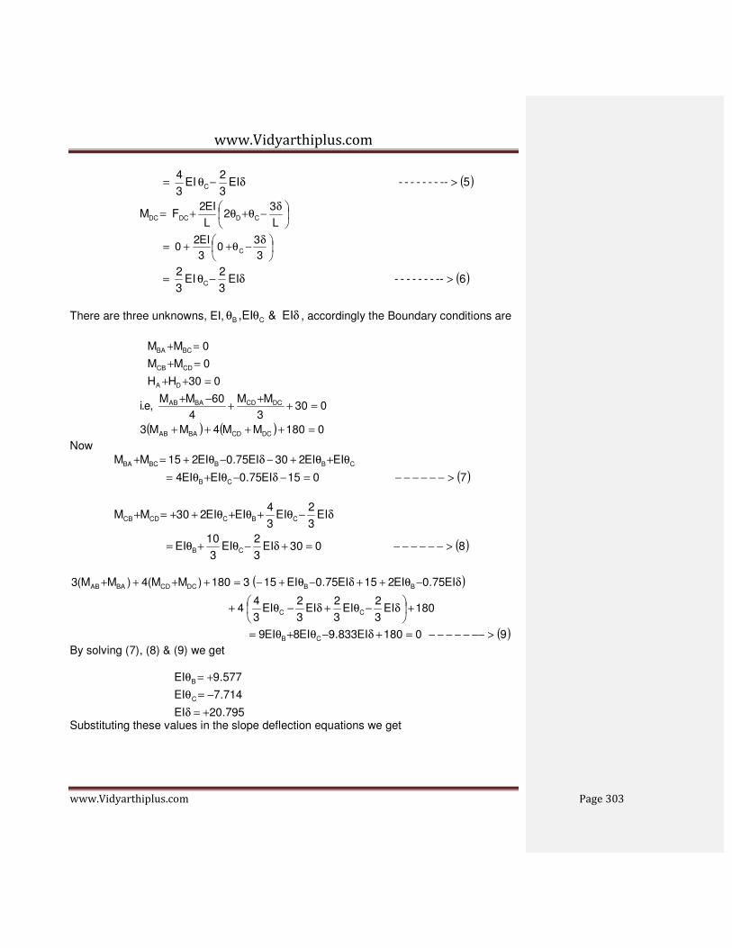
www.Vidyarthiplus.com
www.Vidyarthiplus.com Page 303
( ) 5--------- EI 3
2 EI
3
4 C >δ−θ=
δ−θ+θ+=
L
32
L
EI2F M CDDCDC
3
30
3
EI2 0 C
δ−θ++=
( ) 6--------- EI 3
2 EI
3
2 C >δ−θ=
There are three unknowns, EI, δθθ EI&EI, CB , accordingly the Boundary conditions are
( ) ( ) 0180MM4MM3
0303
MM
4
60MM ,e.i
030HH
0MM
0MM
DCCDBAAB
DCCDBAAB
DA
CDCB
BCBA
=++++
=++
+−+
=++
=+
=+
Now
( )7015EI75.0EIEI4
EIEI230EI75.0EI215MM
CB
CBBBCBA
>−−−−−−=−δ−θ+θ=
θ+θ+−δ−θ+=+
( )8030EI3
2EI
3
10EI
EI3
2EI
3
4EIEI230MM
CB
CBCCDCB
>−−−−−−=+δ−θ+θ=
δ−θ+θ+θ++=+
( )
( )90180EI833.9EI8EI9
180EI3
2EI
3
2EI
3
2EI
3
44
EI75.0EI215EI75.0EI153180)MM(4)MM(3
CB
CC
BBDCCDBAAB
>−−−−−−−=+δ−θ+θ=
+
δ−θ+δ−θ+
δ−θ++δ−θ+−=++++
By solving (7), (8) & (9) we get
795.20EI
714.7EI
577.9EI
C
B
+=δ
−=θ
+=θ
Substituting these values in the slope deflection equations we get

www.Vidyarthiplus.com
www.Vidyarthiplus.com Page 304
( )( ) ( )( )
( )
( )
( ) KNM 00.19795.203
2)714.7(
3
2M
KNM 15.24795.203
2)714.7(
3
4M
KNM 15.24577.9714.7230M
KNM 18.55- 7.714-9.577230- M
KNM55.18795.2075.0577.9215M
KNM 01.21 795.2075.0577.915M
DC
CD
CB
BC
BA
AB
−=−−=
−=−−=
=+−+=
=+=
=−++=
−=−+−=
Reactions: Consider free body diagrams of the members

www.Vidyarthiplus.com
www.Vidyarthiplus.com Page 305
Member AB:
KN615.154
23001.2155.18HA −=
×−−=
-ve sign indicates the direction of HA is from right to left. Member BC:
KN40.3160.28R60R
KN60.284
15.2426055.18R
BC
B
==−=
=−×+
=
Member CD:
KN38.143
15.2419HD =
+=
Check:
ΣH = 0 HA + HD + 30 = 0 -15.62 – 14.38 + 30 = 0 Hence okay

www.Vidyarthiplus.com
www.Vidyarthiplus.com Page 306
Example: Analyse the frame using slope deflection method and draw the Bending
Moment Diagram.
Solution: Assume sway towards right
It can be observed from figure in that direction of moments due to sway in
member AB are anticlockwise and that for member CD are clockwise. Wise shall be
taken to incorporate the same in the slope deflection equation.

www.Vidyarthiplus.com
www.Vidyarthiplus.com Page 307
FEMS
0 Here
M KN 3212
wIF
MKN 3212
424-
12
wIF
DA
2
CB
2
2
BC
=θ=θ
+=+=
−=×
=
−=
Slope deflection equations are:
( )
( )2EI3
2EI
3
4
3
32
3
EI2
L
32
L
EI2FM
1------- EI3
2EI
3
2
3
3
3
EI2
L
32
L
EI2FM
B
B
ABBABA
B
B
BAABAB
>−−−−−δ−θ=
δ−θ=
δ−θ+θ+=
>δ−θ=
δ−θ=
δ−θ+θ+=

www.Vidyarthiplus.com
www.Vidyarthiplus.com Page 308
( )
( )
( )
( )
( )
( )
( )5EI3
2EI
3
4
3
32
3
2EI
L
32
L
EI2FM
4-------- EIEI232
24
I2E232
2L
EI2FM
3--------- EIEI232
24
I2E232
2L
EI2FM
C
C
DCCDCD
BC
BC
BCCBCB
CB
CB
CBBCBC
>−−−−−δ+θ=
δ+θ=
δ+θ+θ+=
>θ+θ++=
θ+θ++=
θ+θ+=
>θ+θ+−=
θ+θ+−=
θ+θ+=
( )6-------- EI3
2EI
3
2
3
3
3
EI2
L
32
L
EI2FM
C
C
CDDCDC
>δ+θ=
δ+θ=
δ+θ+θ+=
The unknown are &, C,B δθθ are conditionsboundary they Accordingl
090MMMM
0303
MM
3
MM,e.i
030HH
0MM
0MM
DCCDBAAB
DCCDBAAB
DA
CDCB
BCBA
=+−−+
=++
−+
=+−
=+
=+
( )7032EI3
2EIEI
3
10
EIEI232EI3
2EI
3
4MM,Now
CB
CBBBCBA
>−−−−−=−δ−θ+θ=
θ+θ+−δ−θ=+

www.Vidyarthiplus.com
www.Vidyarthiplus.com Page 309
( )8032EI3
2EI
3
10EI
EI3
2EI
3
4EIEI232MM
CB
CBCCDCB
>−−−−−=+δ+θ+θ=
δ+θ+θ+θ++=+
( )9045EI3
4EIEI
90EI3
8EI2EI2
90EI3
2EI
3
2EI
3
2
EI3
4EI
3
2EI
3
4EI
3
2EI
3
290MMMM
CB
CB
C
CBBDCCDBAAB
>−−−−−=+δ−θ−θ=
+δ−θ−θ=
+δ−θ−δ−
θ−σ−θ+δ−θ=+−−+
From (7) & (9)
( )10------- 0109EI3EI3
17
045EI3
4EIEI
064EI3
4EI2EI
3
20
CB
CB
CB
>=−θ+θ
=+δ−θ−θ
=−δ−θ+θ
By (8) and (9)
( )11 -------- 0109EI3
17EI3
045EI3
4EIEI
064EI3
4EI
3
20EI2
CB
CB
CB
>=+θ+θ
=+γ−θ−θ
=+δ+θ+θ
By (10) & (11)
071.166EI317
208
071.57EI3EI17
27
0109EI3EI3
17
B
CB
CB
=−θ×
=+θ+θ
=−θ+θ
88.40208
31771.166EI B +=
××=θ
From (10)

www.Vidyarthiplus.com
www.Vidyarthiplus.com Page 310
88.40EI3
17109
3
1EI BC −=
θ−=θ
From (9)
[ ]
( )[ ] 07.954588.4088.404
3
45EIEI4
3EI CB
+=+−−=
+θ−θ=δ
Thus 07.95EI,88.40EI,88.40EI CB =δ−=θ=θ∴
Substituting these values in slope deflection equations
( ) ( )
( ) ( )
( ) ( )( ) ( )
( ) ( )
( ) ( ) KNM12.3607.953
288.40
3
2M
KNM88.807.953
288.40
3
4M
KNM88.888.4088.40232M
KNM88.888.4088.40232M
KNM88.807.953
288.40
3
4M
KNM12.3607.953
288.40
3
2M
DC
CD
CB
BC
BA
AB
+=+−=
+=+−=
−=+−++=
=−++−=
−=−=
−=−=
To find the reaction consider the free body diagram of the frame

www.Vidyarthiplus.com
www.Vidyarthiplus.com Page 311
Reactions: Column AB
KN153
12.3688.8HA =
+=
Beam AB
KN484
2
442488.888.8
RB =××+−+
=
∴ KN4848424RC =−×=
Column CD
KN153
12.3688.8HD =
+=
Check ΣH = 0 HA + HD +P = 0
-15 – 15 + 30 = 0 Hence okay

www.Vidyarthiplus.com
www.Vidyarthiplus.com Page 312
V-UNIT MOMENT DISTRIBUTION METHOD
Advantages of Fixed Ends or Fixed Supports
1. Slope at the ends is zero.
2. Fixed beams are stiffer, stronger and more stable than SSB.
3. In case of fixed beams, fixed end moments will reduce the BM in each section.
4. The maximum defection is reduced.
MOMENT DISTRIBUTION METHOD
MOMENT DISTRIBUTION METHOD -
INTRODUCTION AND BASIC PRINCIPLES
Introduction
(Method developed by Prof. Hardy Cross in 1932)
The method solves for the joint moments in continuous beams and
rigid frames by successive approximation
Statement of Basic Principles
Consider the continuous beam ABCD, subjected to the given loads,
as shown in Figure below. Assume that only rotation of joints occur
at B, C and D, and that no support displacements occur at B, C and
D. Due to the applied loads in spans AB, BC and CD, rotations occur at B, C and D.

www.Vidyarthiplus.com
www.Vidyarthiplus.com Page 313
150KN
In order to solve the problem in a successively approximating manner,
it can be visualized to be made up of a continued two-stage problems
viz., that of locking and releasing the joints in a continuous sequence.
The joints B, C and D are locked in position before any load is applied on the beam ABCD;
then given loads are applied on the beam. Since the joints of beam ABCD are locked in
position, beams AB, BC and CD acts as individual and separate fixed beams, subjected to
the applied loads; these loads develop fixed end moments.
In beam AB
Fixed end moment at A = -wl2/12 = - (15)(8)(8)/12 = - 80 kN.m
Fixed end moment at B = +wl2/12 = +(15)(8)(8)/12 = + 80 kN.m
In beam BC
Fixed end moment at B = - (Pab2)/l
2 = - (150)(3)(3)
2/6
2
= -112.5 kN.m
Fixed end moment at C = + (Pab2)/l
2 = + (150)(3)(3)
2/6
2
= + 112.5
In beam AB
Fixed end moment at C = -wl2/12 = - (10)(8)(8)/12 = - 53.33 kN.m
Fixed end moment at D = +wl2/12 = +(10)(8)(8)/12 = + 53.33kN.m
Since the joints B, C and D were fixed artificially (to compute the the fixed-end moments), now
the joints B, C and D are released and allowed to rotate. Due to the joint release, the joints rotate
maintaining the continuous nature of the beam. Due to the joint release, the fixed end moments

www.Vidyarthiplus.com
www.Vidyarthiplus.com Page 314
on either side of joints B, C and D act in the opposite direction now, and cause a net unbalanced
moment to occur at the joint.
These unbalanced moments act at the joints and modify the joint moments at B, C and D,
according to their relative stiffnesses at the respective joints. The joint moments are distributed
to either side of the joint B, C or D, according to their relative stiffnesses. These distributed
moments also modify the moments at the opposite side of the beam span, viz., at joint A in span
AB, at joints B and C in span BC and at joints C and D in span CD. This modification is
dependent on the carry-over factor (which is equal to 0.5 in this case);
The carry-over moment becomes the unbalanced moment at the joints to which they are
carried over. Steps 3 and 4 are repeated till the carry-over or distributed moment becomes
small.
Sum up all the moments at each of the joint to obtain the joint moments.
SOME BASIC DEFINITIONS
In order to understand the five steps mentioned in section 7.3, some words need to be defined
and relevant derivations made.
7.3.1 Stiffness and Carry-over Factors
Stiffness = Resistance offered by member to a unit displacement or rotation at a point, for given
support constraint conditions

www.Vidyarthiplus.com
www.Vidyarthiplus.com Page 315
A clockwise moment MA is applied at A to produce a +ve bending in beam AB. Find θA and MB.
Using method of consistent deformations
Considering moment MB,
MB + MA + RAL = 0
∴∴∴∴MB = MA/2= (1/2)MA
Carry - over Factor = 1/2

www.Vidyarthiplus.com
www.Vidyarthiplus.com Page 316
7.3.2 Distribution Factor
Distribution factor is the ratio according to which an externally applied unbalanced moment M at
a joint is apportioned to the various members mating at the joint
M = MBA + MBC + MBD
Modified Stiffness Factor
The stiffness factor changes when the far end of the beam is simply-supported.
( )
( )
MFDMK
KM
MFDMK
KM
Similarly
MFDMK
KKM
K
M
KKK
M
KKK
L
IE
L
IE
L
IE
BDBD
BD
BCBC
BC
BABA
BBABA
BDBCBA
B
BBDBCBA
B
).(
).(
).(
444
3
33
2
22
1
11
=
=
=
=
=
==
=++
=∴
++=
+
+
=
∑
∑
∑
∑
θ
θ
θ
θ
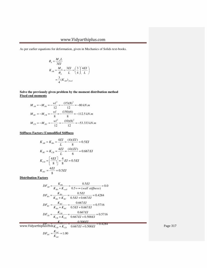
www.Vidyarthiplus.com
www.Vidyarthiplus.com Page 317
As per earlier equations for deformation, given in Mechanics of Solids text-books.
Solve the previously given problem by the moment distribution method
Fixed end moments
Stiffness Factors (Unmodified Stiffness
Distribution Factors
fixedAB
A
AAB
AA
K
L
EI
L
EIMK
EI
LM
)(4
3
4
4
33
3
=
===
=
θ
θ
mkNwl
MM
mkNwl
MM
mkNwl
MM
DCCD
CBBC
BAAB
.333.5312
)8)(10(
12
.5.1128
)6)(150(
8
.8012
)8)(15(
12
22
22
−=−=−=−=
−=−=−=−=
−=−=−=−=
EIEI
K
EIEIEI
K
EIEI
L
EIKK
EIEI
L
EIKK
DC
CD
CBBC
BAAB
5.08
4
5.08
4
8
4
667.06
))(4(4
5.08
))(4(4
==
==
=
====
====
00.1
4284.0500.0667.0
500.0
5716.0500.0667.0
667.0
5716.0667.05.0
667.0
4284.0667.05.0
5.0
0.0)(5.0
5.0
==
=+
=+
=
=+
=+
=
=+
=+
=
=+
=+
=
=∞+
=+
=
DC
DCDC
CDCB
CDCD
CDCB
CBCB
BCBA
BCBC
BCBA
BABA
wallBA
BAAB
K
KDF
EIEI
EI
KK
KDF
EIEI
EI
KK
KDF
EIEI
EI
KK
KDF
EIEI
EI
KK
KDF
stiffnesswall
EI
KK
KDF
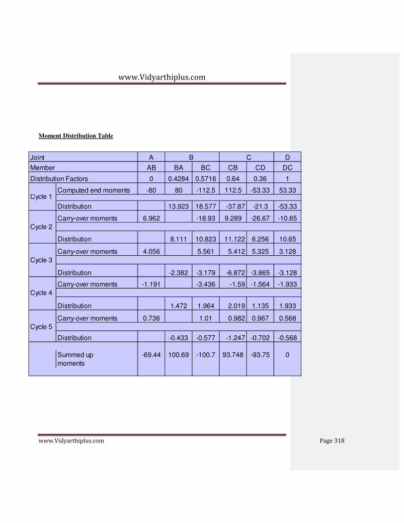
www.Vidyarthiplus.com
www.Vidyarthiplus.com Page 318
Moment Distribution Table
Computation of Shear Forces
Joint A B C D
Member AB BA BC CB CD DC
Distribution Factors 0 0.4284 0.5716 0.64 0.36 1
Computed end moments -80 80 -112.5 112.5 -53.33 53.33Cycle 1
Distribution 13.923 18.577 -37.87 -21.3 -53.33
Carry-over moments 6.962 -18.93 9.289 -26.67 -10.65
Cycle 2
Distribution 8.111 10.823 11.122 6.256 10.65
Carry-over moments 4.056 5.561 5.412 5.325 3.128
Cycle 3
Distribution -2.382 -3.179 -6.872 -3.865 -3.128
Carry-over moments -1.191 -3.436 -1.59 -1.564 -1.933
Cycle 4
Distribution 1.472 1.964 2.019 1.135 1.933
Carry-over moments 0.736 1.01 0.982 0.967 0.568
Cycle 5
Distribution -0.433 -0.577 -1.247 -0.702 -0.568
Summed up -69.44 100.69 -100.7 93.748 -93.75 0
moments
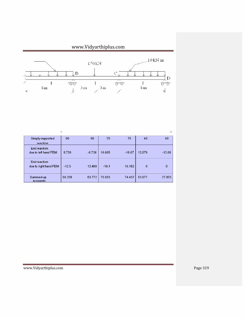
www.Vidyarthiplus.com
www.Vidyarthiplus.com Page 319