© 2014 Samuel O’Neill Skinner

CELLULAR DECISION MAKING:

FROM PHAGE LAMBDA TO STEM CELLS

BY

SAMUEL O’NEILL SKINNER

DISSERTATION

Submitted in partial fulfillment of the requirements

for the degree of Doctor of Philosophy in Physics

in the Graduate College of the

University of Illinois at Urbana-Champaign, 2014

Urbana, Illinois

Doctoral Committee:

Assistant Professor Thomas E. Kuhlman, Chair

Adjunct Associate Professor Ido Golding, Director of Research

Associate Professor Aleksei Aksimentiev

Professor James M. Slauch

ii

Abstract Cellular decision making is the process by which cells choose among functionally-distinct cell states.

Heritable cell states are typically maintained and stabilized by the activity of specific genes, but cells can

also be induced to switch to alternative states given the appropriate stimulus. Underlying decision making

processes that result in different cell states are temporally regulated gene expression cascades. The

decision-making process for switching between cell states can be biased by environmental factors, or can

be driven solely by biochemical noise due to the stochastic nature of the cell.

The inherent stochastic nature of biochemical reactions in the cell has been highlighted by recent

quantitative single-cell measurements. When examined at the single-cell level, the decision-making process

often appears noisy, where individual cells choose different cell states even when subject to identical

conditions. The mixed outcomes of these decisions have been used to demonstrate that molecular noise can

dominate whole-cell processes. However, there may also exist previously unaccounted-for cell parameters

that affect the decision making process, making the decision appear more random than it really is.

Additionally, the maintenance of a heritable cell state is also subject to the stochastic nature of gene

expression. For example, the gene expression programs associated with stabilized cell states often contain a

self-regulating protein. However, characterization of the effect to which fluctuations in gene expression of

a fate-determining protein modulate the stability of the cell state has not been accomplished.

Questions about the effect of the stochastic nature of gene expression on decision making include: In

the face of gene expression stochasticity, can decision-making processes appear more precise when the

proper variables are taken into account? Does the level of gene expression noise dictate the stability of a

gene expression state? To answer questions such as these, we investigate two systems that exhibit cellular

decision making and cell-state maintenance, bacteriophage lambda and mouse embryonic stem cells.

Bacteriophage lambda (phage lambda) is a bacterial virus that, upon infection of its host bacterium,

Escherichia coli, decides between two alternative pathways: The phage can replicate and kill the host cell,

or it can integrate into the host chromosome and passively replicate as part of the host. This integrated

phage can spontaneously switch to replicate and kill the host either by random chance or induction by

specific stimuli. We investigated this decision-making process of phage lambda via microscopy, at single-

cell and single-phage resolution. We observed that the decision-making process is first made at the level of

individual phages, and then integrated into a whole-cell decision. Additionally, we investigated the stability

of the integrated phage in the replicating host. With single-molecule resolution measurements of gene

activity and the measurements of cell-state switching rates, we were able to determine the relationship

between stochastic gene activity and cell-state stability.

In order to extend these techniques to a higher system, we chose to study mouse embryonic stem cells,

which are often used because they closely resemble human biology. Embryonic stem cells are extracted

from the developing embryo and can be maintained in vitro indefinitely while still remaining pluripotent.

Pluripotency is the ability to assume any cell state in the adult body and is the hallmark of embryonic stem

cells. The molecular mechanisms for the stability of pluripotency have been narrowed to three fate-

iii

determining proteins. Two of these proteins are thought to be tightly regulated, Oct4 and Sox2, while the

third, Nanog, exhibits large variability among the population. Additionally, the level of Nanog has been

correlated with the stability of pluripotency. The reasons for the variability in Nanog level are not known,

but stochastic gene expression has been hypothesized as a possible source. We measured the gene activity

of Oct4 and Nanog and found that while Nanog did exhibit a higher degree of heterogeneity at the mRNA

level, both genes exhibited intermittent transcription activity. Additionally, when we used

phenomenological models to extract the kinetics of transcription, we found that the cause of Nanog’s

higher heterogeneity was due to a slower rate of transcriptional activation.

Our experiments demonstrate that high-resolution measurements paired with modeling of stochastic

processes is a powerful approach for studying cellular decision making. The techniques developed here

allow for better resolution of the precision of cellular decision making by accounting for sources of

measurement noise. Our techniques also give us the ability to connect the stochastic events of gene

expression to the whole-cell phenotypes of cell-state stability.

iv

To my family

v

Acknowledgements

I would like to thank foremost my mentor, Ido Golding, whose enthusiasm for science was a constant

source of inspiration for me throughout my graduate career. I am extremely grateful to have had the

opportunity to work under his guidance and learn from him every day. For me, he has been a model

principal investigator: on the one hand, he always had time to meticulously demonstrate the scientific

method, and on the other hand, he was always fair, professional, and communicated very clearly the goals

of the lab and the expectations he had of his students. I learned early on that the challenges I was to face in

graduate school, namely public speaking, were some that I had been avoiding most of my life. Because of

my initial struggles, I am grateful for Ido’s perseverance as a mentor and teacher. In learning how to

prepare for these challenges, and with time conquer them, I certainly found lessons that extended to other

areas of my life. Towards this accomplishment, I am especially thankful to Ido and my time in his lab.

Additionally, I am grateful to have been surrounded by the many enthusiastic members of the Golding

lab. It has been a great pleasure to get to know them and share the frustrating and exciting experiences of

research. Thanks very much: Tommy So, Chenghang Zong, Lanying Zeng, Michael Bednarz, Lance Min,

Patrick Mears, Leonardo Sepulveda, Eli Rothenberg, Heng Xu, Mengyu Wang, Jing Zhang, and Louis

McLane. I would also like to thank Anna Sokac for being a source of encouragement and friendship and to

have brought such talented members to her lab: Lauren Figard, Liuliu Zheng, and Zenghui Xue.

I would like to thank the many inspiring instructors in the Physics Department of UIUC for providing

stimulating Physics courses. I was very fortunate to have had instructors that cared deeply to engage their

students and encourage them to think of the course subject matter in insightful ways. I would sincerely like

to thank Nigel Goldenfeld, Gordon Baym, Philip Phillips, and Michael Stone for their passion for teaching.

Additionally, I would like to thank Melodee Schweighart and Lance Cooper for their assistance with the

move to Houston and helping me move swiftly through all bureaucratic details of being a remote student.

I am indebted to my preliminary exam committee: Nigel Goldenfeld, Paul Selvin, and Karen Dahmen,

for their commitment to improving my communication of science. Additionally, I would like to thank my

thesis defense committee: Thomas Kuhlman, Aleksei Aksimentiev, and James Slauch, for participating in a

challenging and interesting defense.

I consider myself very fortunate to have been a part of the Center for Physics of the Living Cells. This

center provided such a stimulating environment for collaborative research. I look forward to seeing the

future of projects it produces, and hope to continue to collaborate with its members for years to come. From

CPLC, I would particularly like to thank the inspiring investigators and administrators: Taekjip Ha, Paul

Selvin, Yann Chemla, Thomas Kuhlman, Martin Gruebele, Jaya Yodh and Sandra Patterson. Additionally,

I would like to say thanks to the many CPLC summer school teaching assistants and participants who have

enriched that week of my life for the last five years with long dedicated hours, thoughtful questioning, and

enthusiasm.

The Department of Biochemistry and Molecular Biology of Baylor College of Medicine graciously

adopted us UIUC graduate students that moved to Houston with Ido, and allowed us to develop as one of

vi

their own. I am very grateful for this experience, as it provided ample opportunities to practice the

presentation of science and allowed me to explore new avenues of research. I feel very fortunate to have

gotten research experience within both institutions. From Baylor, I would like to thank John Wilson, Ruth

Reeves, Monica Bagos, and the BMB faculty. Additionally, it was wonderful to collaborate with the

Westbrook and Zwaka labs.

I would like to thank my family of friends in Champaign who showed me the ropes of graduate school

and provided me the structure I needed during my initial acclimation. Thanks to Rogan Carr, Christy

Scheuer, Kelsey Keyes, Carl Lehnen, Christine Cohen and Noah Cohen. After moving to Houston, I am

deeply appreciative of my family of friends that helped me through the remainder of graduate school with

new adventures and interesting challenges. Thanks to Diana Jenschke, Lisa Hawkins, Andrew Urie, Megan

Dye, Sarah Edwards, Chris Rybowiak, Mike Evangelista, Ramon Roman, Mike Iannotti, and Dillon Baete.

Lastly, I’d like to thank my amazing family for supporting me through all aspects of graduate school.

I am endlessly indebted to them for encouraging me to improve, supporting me through roadblocks, and

celebrating all accomplishments. I am excited to come back home and share my life with you again.

vii

Table of contents

Part I: Quantitative adventures in the life-cycle of bacteriophage lambda .... 1

1 Background to bacteriophage lambda .......................................................... 2

1.1 The bacteriophage lambda life-cycle ............................................................................... 2

1.2 Bacteriophage lambda as a model system ...................................................................... 3

1.3 Aim of this work .................................................................................................................. 3

2 The post-infection decision in phage lambda .............................................. 4

2.1 Introduction ......................................................................................................................... 4

2.2 Results ................................................................................................................................. 6

Constructing a fluorescent phage ........................................................................................................... 6

Assaying the post-infection decision with single-phage resolution ....................................................... 8

Lysogeny requires a unanimous decision by all infecting phages ......................................................... 9

The precision of the single-phage decision is lost at the single-cell level ............................................11

2.3 Discussion......................................................................................................................... 12

3 Stability of the lysogenic state in phage lambda ....................................... 15

3.1 Introduction ....................................................................................................................... 15

3.2 Results ............................................................................................................................... 16

Single-molecule-resolution characterization of gene activity in a lysogen ...........................................16

Measurement of lysogenic stability ......................................................................................................18

Stability is determined by the frequency of activity bursts from PRM ...................................................19

3.3 Discussion......................................................................................................................... 21

Part II: Measuring transcription kinetics in individual mouse embryonic

stem cells .......................................................................................................... 23

4 Background to mouse embryonic stem cells ............................................. 24

4.1 Introduction to mouse embryonic stem cells ................................................................ 24

Defining features ..................................................................................................................................24

Embryonic stem cell line derivation .....................................................................................................24

4.2 Control of the embryonic stem cell state ....................................................................... 25

viii

Pluripotency and self-renewal are primarily maintained by a small network of transcription factors ..25

Modulation of pluripotency transcription-factor gene expression ........................................................27

Sources of pluripotency transcription-factor heterogeneity ..................................................................27

4.3 Questions addressed in this work .................................................................................. 28

5 Quantifying mRNA copy-number in individual mouse embryonic stem

cells .................................................................................................................... 29

5.1 Single-molecule Fluorescent in situ Hybridization (smFISH) ...................................... 29

Development of the protocol ................................................................................................................29

Overview of the smFISH protocol ........................................................................................................30

Using intron and exon labeling to distinguish nascent and mature mRNA ..........................................31

5.2 Obtaining mRNA copy number from images ................................................................. 31

Automated cell and nucleus recognition ...............................................................................................32

DNA content segmentation ...................................................................................................................32

3D spot recognition ...............................................................................................................................34

Distinguishing real spots from false positives ......................................................................................35

Spot calibration and counting ...............................................................................................................35

Identification of nascent and mature mRNA ........................................................................................36

5.3 Nascent and mature mRNA copy-numbers of Oct4 and Nanog .................................. 36

5.4 Accuracy and dynamic range of smFISH measurements ............................................ 37

5.5 Limitations of smFISH ...................................................................................................... 37

5.6 Summary ........................................................................................................................... 38

6 Extracting transcription kinetics from nascent and mature mRNA copy-

number distributions ........................................................................................ 39

6.1 A stochastic, phenomenological model of transcription including nascent and

mature RNA .............................................................................................................................. 39

Phenomenological models of transcription: Poisson and ‘bursty’ expression ......................................39

Including deterministic elongation of nascent mRNA in the two-state model .....................................41

Nascent and mature mRNA production can be modeled as two processes with equal initiation kinetics

..............................................................................................................................................................42

6.2 Modeling multiple alleles ................................................................................................. 42

6.3 Two-state model with nascent mRNA describes observed nascent and mature copy-

number distributions ............................................................................................................... 43

Kinetic rate calculation by fitting nascent and mature mRNA distributions ........................................43

Comparison of kinetic rates between Oct4 and Nanog .........................................................................45

6.4 Analysis of dosage compensation across the cell cycle .............................................. 45

ix

Gene activity for Oct4 and Nanog does not double after gene replication ...........................................45

6.5 Summary ........................................................................................................................... 47

Glossary ............................................................................................................ 48

Appendix A. Bacteriophage lambda experimental protocols ...................... 50

A.1 Strains, growth media and growth conditions .............................................................. 50

Media and growth conditions ...............................................................................................................50

Bacterial strains ....................................................................................................................................50

Bacteriophage lambda strains ...............................................................................................................51

A.2 Bacteriophage propagation and handling ..................................................................... 53

Titering phage concentration ................................................................................................................53

Mitomycin-C induction of wildtype prophages ....................................................................................53

Heat induction of temperature-sensitive prophages (cI857) .................................................................54

Plate-amplification ................................................................................................................................54

Lysogenization ......................................................................................................................................55

A.3 Quantitative bulk measurements ................................................................................... 56

Lysogenization frequency .....................................................................................................................56

Lysogen spontaneous induction rate .....................................................................................................56

“One-step” burst size measurement ......................................................................................................57

A.4 Genetic manipulation ...................................................................................................... 58

Crossing D-eyfp from a plasmid onto a ʎ-Dam phage ..........................................................................58

A.5 Transmission electron microscopy ............................................................................... 59

Appendix B. Mouse embryonic stem cells experimental protocols ............ 60

B.1 Mouse embryonic stem cell lines and media ................................................................ 60

Cell lines ...............................................................................................................................................60

Media and cell culture...........................................................................................................................60

B.2 Mammalian cell culture ................................................................................................... 61

Reviving frozen stocks..........................................................................................................................61

Passaging ..............................................................................................................................................61

Making liquid nitrogen stocks ..............................................................................................................62

Measuring cell density using a hemocytometer ....................................................................................62

B.3 Single-molecule Fluorescent in situ Hybridization (smFISH) ..................................... 64

Probe design .........................................................................................................................................64

Probe labeling .......................................................................................................................................66

x

Sample fixation and permeabilization ..................................................................................................67

Hybridization ........................................................................................................................................68

Washing ................................................................................................................................................68

B.4 Fluorescence microscopy............................................................................................... 69

Appendix C. Data Analysis ............................................................................. 71

C.1 Spot recognition (Spätzcells) ......................................................................................... 71

Gaussian smoothing ..............................................................................................................................71

Maxima detection in 3D .......................................................................................................................71

2D Gaussian fitting ...............................................................................................................................71

Allocation of spots to cells ....................................................................................................................72

C.2 Finite state projection algorithm .................................................................................... 73

Chemical master equation .....................................................................................................................73

Finite state projection algorithm ...........................................................................................................73

Finite state projection algorithm modified to include deterministic elongation....................................74

Appendix D. Derivation of formulas used in this work ................................. 76

D.1 Proof that the range of input parameters allowing coexistence of cell fates is

inversely proportional to the Hill coefficient ........................................................................ 76

D.2 Theoretical reconstruction of the single-cell and population-averaged

lysogenization phenotypes .................................................................................................... 77

Lysogenization probability of a cell infected by m phages ...................................................................77

Lysogenization probability in bulk experiments ...................................................................................78

D.3 Expression for the lysogen spontaneous induction rate ............................................ 79

References ........................................................................................................ 80

1

Part I: Quantitative adventures in the life-cycle of bacteriophage lambda

2

1 Background to bacteriophage lambda

In this chapter, I will describe bacteriophage lambda, the model system used in our work, which is

explored in Chapters 2-3. Primarily, I will describe the life-cycle of bacteriophage lambda, and how it

displays intriguing features that are also found in higher organisms. In the following chapters, I will

describe our efforts to build a quantitative narrative of the bacteriophage lambda life-cycle, and how

specific features found in this simple system relate to higher level systems.

1.1 The bacteriophage lambda life-cycle

Bacteriophage lambda (phage lambda; Fig. 1.1) is a

bacterial virus that infects Escherichia coli (E. coli) (Hendrix,

1983; Hershey, 1971; Ptashne, 2004). Viruses are

metabolically inactive particles that replicate by appropriating

the gene-expression machinery of their hosts, typically killing

the host cell in the process. The life cycle starts with phage

lambda passively diffusing in the environment, until finding a

specific receptor on the surface of an E. coli cell. Phage

lambda will then bind to the receptor and inject its genome

into the host cell. After DNA injection, the virus hijacks the

metabolism of the host, and will begin a temporally regulated

cascade of viral gene-expression. Depending on a few

parameters of the infection, gene-expression will ultimately be

directed to one of two distinct viral replication pathways: lysis

or lysogeny (Golding, 2011; Oppenheim et al., 2005; Ptashne,

2004; Weitz et al., 2008; Zeng et al., 2010) (Fig. 1.2).

In the lytic pathway, viral proteins responsible for phage DNA replication, phage structure, and host

cell death (lysis) are produced. After production, structural phage proteins self-assemble and package

replicated viral genomes to create phage progeny. After cell lysis, ~200 progeny phages will be released

into the environment to begin the cycle anew (Ptashne, 2004; Zeng et al., 2010; Zong et al., 2010).

In the lysogenic pathway, further viral gene expression is repressed and the viral genome is integrated

into the bacterial chromosome. The integrated viral genome is then replicated as part of the host’s

chromosome and is passed to each daughter cell (Ptashne, 2004; Ptashne, 2007). Cells that contain a

dormant phage in their genomes are called lysogens. About 45 minutes after infection, phage lambda will

have ‘chosen’ one of the two distinct pathways and the host cell will exhibit the corresponding phenotype:

either cell death releasing progeny phages, or a dormant phage residing in a host cell (Kobiler et al., 2005;

Oppenheim et al., 2005).

Figure 1.1. Transmission Electron

Microscopy (TEM) of bacteriophage lambda.

Lambda has an icosahedral capsid (~50 nm in

diameter) containing the viral DNA. Its tail

(~150 nm in length) injects DNA through

receptors on the surface of an E. coli cell. I

optimized the protocol for investigating phage

morphology under TEM (see Appendix A.5).

3

The lysogenic state remains stable

through the activity of a single viral

protein, the lambda repressor (CI). The

lambda repressor is a transcription

factor that binds to DNA and maintains

its own expression, as well as represses

all other viral gene expression and

functions. This lysogenic state is

extremely stable, only spontaneously

switching to lysis once in 108

generations (Little et al., 1999).

However, the integrated phage can be

quickly and efficiently induced to

switch in response to the proper

environmental stimulus (e.g. host DNA

damage (Chia et al., 2009; Ptashne,

2004)).

1.2 Bacteriophage lambda as a model system

We use phage lambda as a model system because, despite its relative simplicity (48.5 kbp genome

encoding ~50 genes), it exhibits phenomena relevant for higher biological systems including:

Developmental pathway selection as exhibited during the post-infection decision.

Long-term memory of a gene expression state.

Fast and efficient cell-state switching in response to the proper stimulus.

For phage lambda, the components that make up these phenomena are well understood at the genetic

and biochemical level. However, a quantitative and predictive narrative connecting biochemical events to

whole-cell phenotypes has not been accomplished.

1.3 Aim of this work

In the following chapters, I will describe our efforts to build quantitative narratives for developmental

decision-making (Chapter 2) and the maintenance of a cell state (Chapter 3) in the lambda system. To

that end, we aim to characterize these phenomena at the single-cell and single-phage level. These studies

reveal simple underlying principles that can be applied to higher systems.

Figure 1.2. Bacteriophage lambda life-cycle

Phage lambda infects an E. coli cell by finding its target on the cell surface

and delivering its genome into the cell. After infection, the phage will decide

to replicate through lysis or lysogeny. The lysis pathway will produce ~200

progeny phages and kill the host cell. The lysogeny pathway will produce a

lysogen cell, where the lambda genome has been incorporated into the

bacterial genome and will be passed to daughter cells. The phage genome is

extremely stable within the lysogen cell, but can quickly and efficiently

switch to lysis in response to the proper stimulus.

4

2 The post-infection decision in phage lambda

In this chapter, I will describe how we used our model system, bacteriophage lambda, to investigate

cellular decision making (cell-fate determination) beyond the resolution of individual cells. When the

process of cell-fate determination is examined at single-cell resolution, it is often observed that individual

cells undergo different fates even when subject to identical conditions. This ‘noisy’ phenotype is usually

attributed to the inherent stochasticity of chemical reactions in the cell. Here we demonstrate how the

observed single-cell heterogeneity can be explained by a cascade of decisions occurring at the subcellular

level. We follow the post-infection decision in bacteriophage lambda at single-virus resolution, and show

that a choice between lysis and lysogeny is first made at the level of the individual virus. The decisions by

all viruses infecting a single cell are then integrated in a precise (noise-free) way, such that only a

unanimous vote by all viruses leads to the establishment of lysogeny. By detecting and integrating over the

subcellular ‘hidden variables,’ we are able to predict the level of noise measured at the single-cell level.

Parts of this chapter are taken from our paper, “Decision Making at a Subcellular Level Determines

the Outcome of Bacteriophage Infection.” (Zeng L, Skinner SO, Zong C, Sippy J, Feiss M, and Golding I.

Cell 141, 682-91 (2010)). All results shown are mine unless otherwise stated.

2.1 Introduction

Living cells integrate signals from their environment to make fate-determining decisions (Alon,

2007). When examined at the single-cell level, the process of cellular decision-making often appears

imprecise or ‘noisy,’ in the sense that individual cells in a clonal population undergo different fates even

when subject to identical conditions (Arkin et al., 1998; Blake et al., 2006; Blake et al., 2003; Chang et al.,

2008; Elowitz and Leibler, 2000; Kaern et al., 2005; Losick and Desplan, 2008; Maamar et al., 2007; Singh

and Weinberger, 2009; Spencer et al., 2009; Suel et al., 2007; Yamanaka, 2009). In the literature, this cell-

fate heterogeneity has largely been attributed to the inherent stochasticity of chemical reactions in the cell,

especially the reactions governing gene expression (Losick and Desplan, 2008; Raj and van Oudenaarden,

2008; Singh and Weinberger, 2009). In recent years, considerable progress has been made toward

understanding the sources and characteristics of this stochasticity. For example, the fact that both

transcription (Chubb et al., 2006; Golding et al., 2005; Raj et al., 2006) and translation (Cai et al., 2006; Yu

et al., 2006) occur in a bursty, non-Poissonian manner implies that cell-to-cell variations in protein levels

are higher than previously assumed. In another line of investigation, the role of stochastic gene expression

in cell-fate decisions has been directly demonstrated and quantified (Cagatay et al., 2009; Maamar et al.,

2007; Suel et al., 2007).

At the same time, however, a competing view regarding the source of cell-fate heterogeneity is that

what seems like an imprecise decision by the cell may largely reflect our own inability to measure some

‘hidden variables,’ i.e., undetected differences between individual cells, which deterministically set the

5

outcome of cellular decision making. As two recent works have shown (Snijder et al., 2009; St-Pierre and

Endy, 2008), careful quantification of cell-to-cell differences can in some cases ‘explain away’ some—but

not all—of the observed cell-fate heterogeneity without the need to invoke chemical stochasticity. So far,

the two lines of evidence regarding cell-fate heterogeneity have existed in parallel, and have not been

reconciled within a single quantitative narrative of how stochasticity and ‘hidden variables’ combine to

produce the observed single-cell phenotype.

Here we use the decision between dormancy (lysogeny) and cell death (lysis) following infection of

E. coli by bacteriophage lambda to demonstrate how a cascade of decisions at the subcellular level gives

rise to the ‘noisy’ phenotype observed at the single-cell level. We follow viral infection at the level of

individual phages and cells. We find that, upon infection of the cell by multiple phages, a choice between

lysis and lysogeny is first made at the level of each individual phage dependent on the total viral

concentration inside the cell. The decisions by all viruses infecting a single cell are then integrated in a

precise (noise-free) way, such that only a unanimous ‘vote’ by all viruses leads to the establishment of

lysogeny. By integrating over the subcellular degrees of freedom (number and location of infecting phages,

cell volume), we are able to reproduce the observed whole-cell phenotype and predict the observed level of

noise in the lysis/lysogeny decision.

Upon infection of an E. coli cell by bacteriophage lambda, a decision is made between cell death

(lysis) and viral dormancy (lysogeny) (Ptashne, 2004), a process that serves as a simple paradigm for

decision-making between alternative cell fates during development (Court et al., 2007). During the decision

process, the regulatory circuit encoded by viral genes (primarily cI, cII, and cro) integrates multiple

physiological and environmental signals, including the number of infecting viruses and the metabolic state

of the cell, in order to reach a decision (Oppenheim et al., 2005; Weitz et al., 2008). More than a decade

ago, Arkin and coworkers (Arkin et al., 1998) used a numerical study of the lambda lysis/lysogeny decision

following infection to emphasize the role of stochasticity in genetic circuits. Their work led to the

emergence of the widely accepted picture of cell variability driven by spontaneous biochemical

stochasticity, not only in lambda (Arkin et al., 1998; Singh and Weinberger, 2009) but in other systems as

well (Chang et al., 2008; Losick and Desplan, 2008; Maamar et al., 2007; Singh and Weinberger, 2009;

Suel et al., 2007). More recently, however, it was shown by St-Pierre and Endy that, at the single-cell level,

cell size is correlated with cell fate following lambda infection, thus explaining away some of the observed

cell-fate heterogeneity and reducing, though not eliminating, the expected role of biochemical stochasticity

in the decision (St-Pierre and Endy, 2008).

For the purpose of deconstructing the lambda post-infection decision, a few candidates should be

considered as possible hidden microscopic parameters affecting cell fate. The number of phages infecting

an individual cell (multiplicity of infection; MOI) has long been known to affect cell fate (Kourilsky and

Knapp, 1974), although the quantitative form of this dependence has been unclear (Kourilsky and Knapp,

1974). In addition, recent results suggest that both the volume of the infected cell (St-Pierre and Endy,

2008) and the position of the infecting phages on the cell surface (Edgar et al., 2008) may be important.

6

Some or all of these parameters are hidden from us, not only in bulk experiments but also in single-cell

assays where the individual infecting viruses cannot be tracked (St-Pierre and Endy, 2008). We thus set out

to examine the infection process at the level of individual phages and cells at a spatiotemporal resolution

sufficient to quantify the relevant subcellular parameters. This allowed us, in turn, to evaluate the

contribution of each factor to the observed cell-fate heterogeneity.

2.2 Results

Constructing a fluorescent phage

To enable detection of individual phages, we first constructed a fluorescently labeled lambda strain,

λLZ1, in which the viral capsid is made purely of a fusion protein of head-stabilization protein gpD and

yellow fluorescent protein (EYFP), gpD-EYFP (Alvarez et al., 2007). λLZ1 was found to exhibit multiple

phenotypic problems. First, when performing phage purification, the titer successively decreased. For

example, after purification of the crude lysate through the precipitation with polyethylene glycol (PEG) in

the presence of high salt (Sambrook and Russell, 2001), the λLZ1 titer decreased from ~109 plaque forming

Figure 2.1. Obtaining a fluorescent phage phenotypically identical to wildtype lambda.

Bulk assay for lysogenization probability as a function of MOI. Δ: Wildtype (λIG2903); ○: gpD-mosaic (λLZ2); □: gpD-

EYFP (λLZ1); ◊: gpD-EYFP (λSOS2). Lines: Theoretical predictions based on Poisson collision statistics between

individual bacteria and phages combined with a single-cell lysogenization response where lysogeny requires

infection by: two or more phages (m≥2; blue), and one or more phages (m≥1; red). The experimental data was shifted

to accommodate for the imperfect adsorption and infection efficiencies. The gpD-mosaic phage exhibits the same

MOI-response as wildtype. Both gpD-EYFP phages exhibit different MOI-response phenotypes when compared to

wildtype.

7

units per ml (pfu/ml) to ~108 pfu/ml, whereas for the wildtype phage (λIG2903), titer typically increased 20-

fold. Second, we examined the λLZ1 morphology using electron microscopy (see Appendix A.5 for the

detailed protocol). As is typical of a crude lysate, particles were not uniform in size and shape. In addition,

many empty viral capsids were seen (data not shown). The unavailability of a purified stock prevented us

from performing a more qualitative analysis of phage morphology, as was done for wildtype and the gpD-

mosaic phage (see below). Third, we measured the lysogenization probability as a function of MOI

(multiplicity of infection). The lysogenization probability was plotted as a function of MOI on a log-log

scale (Fig. 2.1). It was found that λLZ1 exhibited a different MOI-response than wildtype.

To test the hypothesis that other mutations in the λLZ1 genome were the source of these problems, we

engineered a gpD-EYFP phage (λSOS2) that was otherwise wildtype. Briefly, D-eyfp was PCR amplified

using λLZ1 as a template. Primers were designed to amplify ~650bp upstream and downstream of D-eyfp,

regions homologous to wildtype lambda. Homologous recombination was used to integrate the PCR

product into ʎsus123 [Dam123] (gift of Allan Campbell, Stanford University), where D-eyfp replaced the

amber mutated D during this recombination (for detailed protocols, see Appendix A.4). The resulting

phage, λSOS2, was then tested for the phenotypic problems seen in λLZ1. We measured the lysogenization

probability as a function of MOI and found that λSOS2 had the same MOI response as λLZ1 (Fig. 2.1). We

concluded that a capsid comprised only of gpD-EYFP proteins produced the observed deviations from

wildtype behavior.

We decided to construct a gpD-mosaic phage (λLZ2), inspired by a previous work (Zanghi et al., 2005)

that showed stable phage assembly when wildtype and recombinant versions of gpD capsid proteins were

coexpressed. The λLZ2 phage capsid contains a mixture of the wildtype gpD and gpD-EYFP. These ‘mosaic-

YFP’ phages were detectable as diffraction-limited objects under epifluorescent illumination. The presence

of fluorescent proteins in the viral capsids did not perturb the phage phenotype: the phage capsid

morphology was indistinguishable from wildtype (Fig. 2.2); they packed viral DNA at close to 100%

efficiency (data not shown); and, most importantly, their lysogenization phenotype, as measured in bulk,

was indistinguishable from that of wildtype phages (Fig. 2.1).

Figure 2.2. Phage morphology examined

using transmission electron microscopy.

The gpD-mosaic phage (λLZ2, left) exhibited

normal phage morphology, indistinguishable

from the wildtype (λIG2903, right).

(Magnification ~100,000x, negative

staining with Nano-W.)

8

Assaying the post-infection decision with single-phage resolution

To characterize the post-infection decision, individual infection events were followed under the

fluorescence microscope (Fig. 2.3). The initial infection parameters were recorded: the number and

positions of phages infecting each individual cell, as well as the size of the infected cell. Time-lapse

microscopy was then used to examine the fate of each infected cell. Choice of the lytic pathway was

evinced by the production of many new fluorescent phages, followed by cell lysis (Fig. 2.3A). Lysogeny

was detected through a transcriptional reporter plasmid expressing mCherry from the PRE promoter, which

controls the establishment of lysogeny (Kobiler et al., 2005) (Fig. 2.3). The presence of this plasmid in

infected cells did not the affect decision-making behavior (data not shown). The majority of infected cells

(75%, 1048/1394 cells, 22 experiments) exhibited either lysis or lysogeny following infection. A small

Figure 2.3. Assaying the post-infection decision with single-phage resolution.

(A) A schematic description of our cell-fate assay. Multiple YFP-labeled phages simultaneously infect individual cells of

E. coli. The post-infection fate can be detected in each infected cell. Choice of the lytic pathway is indicated by the

intracellular production of new YFP-coated phages, followed by cell lysis. Choice of the lysogenic pathway is indicated by

the production of mCherry from the PRE promoter, followed by resumed growth and cell division. The three stages of the

process correspond to the three images seen in (B) below. (B) Frames from a time-lapse movie depicting infection events.

Shown is an overlay of the phase-contrast, mCherry, and YFP channels (YFP channel: sum of multiple z slices for t = 0;

single z slice at later time frames). At t = 0 (left), two cells are seen each infected by a single phage (green spots), and one

cell is infected by three phages. At t = 80 min (middle), the two cells infected by single phages have each gone into the

lytic pathway, as indicated by the intracellular production of new phages (green). The cell infected by three phages has

gone into the lysogenic pathway, as indicated by the production of mCherry from the PRE promoter (red). At t = 2 hr (right),

the lytic pathway has resulted in cell lysis, whereas the lysogenic cell has divided. (Note: a number of unadsorbed phages

were removed from the image for clarity.) Data by L. Zeng.

9

fraction of the infection events (10%, 143/1394 cells) did not lead to either lysis or lysogeny, and cells

resumed normal growth. As evidence for the fidelity of our infection assay, we observed that infection of

cells that have already been lysogenized, and which should be immune to further infections (Hershey,

1971), indeed resulted in 0% lytic development (0/43 cells; data not shown). On the other hand, infection at

40°C, where the repressor proteins produced by the phages are inactivated (Hecht et al., 1983; Hershey,

1971), led to 100% lysis (50/50 cells; data not shown).

We examined the effect of different infection parameters on the resulting cell fate (among cells

undergoing lysis or lysogeny; Fig. 2.3B). In agreement with bulk experiments ((Kourilsky and Knapp,

1974) and Fig. 2.1), the probability of lysogeny f increased with the number of phages m infecting an

individual cell (MOI). The probability f approached ~1 (100% lysogeny) when m was sufficiently large. To

characterize the imprecision of the observed decision, we fit f(m) to a Hill function (Alon, 2007),

. The Hill coefficient h can then be used as a phenomenological indicator for the decision

precision: the range of input parameters Δm for which both fates can be observed is proportional to 1/h (see

Appendix D.1 for derivation). Thus, the higher h, the higher the chance of observing a unique cell fate

(less cell-fate heterogeneity is observed), and the decision can be said to be more precise (less noisy). For

f(m), we find h ≈ 1 (h = 1.00 ± 0.10 [SEM], 1706 cells). As we show below, characterizing the lysogeny

decision at the level of individual infecting phages reveals a much sharper (less noisy) decision. Another

factor affecting the decision is the length of the infected cell (which serves as a metric for both its age

(Neidhardt et al., 1990) and its volume). Shorter cells exhibited a higher propensity to lysogenize. This

result complements previous results obtained at m = 1, in which cell fate was shown to be correlated with

cell volume (discussed below) (St-Pierre and Endy, 2008).

Lysogeny requires a unanimous decision by all infecting phages

Previous studies (St-Pierre and Endy, 2008; Weitz et al., 2008) have suggested that the relevant

parameter affecting cell fate is not the absolute number of infecting phages m but rather the ‘viral

concentration’ m/V, where V is the cell volume. This suggestion is based on the observation that m/V

determines the dosage of viral-encoded genes, which in turn governs the post-infection decision (Weitz et

al., 2008). To examine this hypothesis, we mapped the dependence of f on both cell length l (a proxy for

cell volume) and multiplicity-of-infection m (Fig. 2.4A). If the viral-concentration hypothesis is correct,

then f(m,l) should be a function of m/l only. Thus, for example, the chance of lysogenization will be the

same for a single phage infecting a cell of length l0 as for two phages infecting a cell of length 2l0. As seen

in Fig. 2.4A, however, this is not the case. When plotting f versus m/l, the f values for different ms do not

fall on the same line. Specifically, the curves become flatter for higher MOIs. To explain this behavior, we

note that the (m/l) scaling is based on the assumption of a single decision made at the whole-cell level. The

possibility of an earlier ‘subcellular’ step, namely that of an independent (possibly noisy) decision by each

infecting phage, is not included. To incorporate this feature, we examined the following hypothesis: when

10

m phages infect a cell, each phage independently chooses between lysis and lysogeny. The probability of an

individual phage choosing the lysogenic pathway (denoted f1) depends on the viral concentration alone, and

is thus given by f1 = f1(m/l). There is still a finite probability (1 - f1) that the phage will choose the lytic

pathway. The expression of lytic genes from a single phage will in turn activate the lytic pathway response

in the whole cell, since this pathway is the default state of the lysis/lysogeny switch (Court et al., 2007;

Oppenheim et al., 2005). In contrast, for the lysogenic pathway to be chosen in the cell, all m phages have

to choose lysogeny, an event that will happen with a probability [f1]m. We therefore expect, for a cell

infected by m phages, that f(m,l) = [f1(m/l)]m. As seen in Fig. 2.4B, this turns out to be the case. Plotting

[f(m,l)](1/m)

versus (m/l) collapses the data from different MOIs into one curve.

The functional form revealed by Fig. 2.4B, f(m,l) = [f1(m/l)]m, should be understood as follows: f1(m/l)

is the probability of an individual phage choosing lysogeny, given that a cell of length l has been infected

by m phages. This function is sigmoidal in (m/l), reflecting the fact that, for each infecting phage, the

probability of lysogenization increases sharply with the viral concentration inside the cell. Note that,

compared to the single-cell response f(m), the single-phage ‘decision curve’ displays a sharper threshold

behavior, i.e., is less noisy. When fitted to a Hill function, the Hill coefficient obtained is h = 2.07 ± 0.11

(standard error) (compared to h = 1.0 ± 0.10 (standard error) observed at the whole-cell level). This

threshold behavior obviously could not have been unveiled were our measurements limited to the

resolution of individual cells but not individual viruses. The whole-cell lysogenization probability f(m,l)

scales like the single-phage probability f1(m/l) to the power m. This scaling indicates that only if all m

phages infecting a cell choose lysogeny is that fate followed. Thus, once each phage has made its (noisy)

Figure 2.4. Lysogeny requires a unanimous decision by all infecting phages.

(A) Probability of lysogeny f as a function of viral concentration (m/l). The data from different MOIs (filled squares, different

colors) do not collapse into a single curve, but instead can be fitted to the separate curves f(m,l). (B) Scaled probability of

lysogeny ([f(m,l)]1/m) as a function of viral concentration (m/l). Data from different MOIs (filled squares, different colors)

collapse into a single curve, representing the probability of lysogeny for each individual infecting phage (f1), in a cell of length l

infected by a total of m phages. f1 can be fitted to a Hill function, f1(m/l) = (m/l)h/(Kh+(m/l)h), with h = 2.07 ± 0.11, K = 1.17 ±

0.02 (SEM). Data by L.Zeng.

11

decision, a precise (noiseless) cellular decision is made based on those individual-phage votes. The logic of

the cellular decision can be thought of as a simple ‘AND’ gate, such that only if all inputs are ‘1’ (i.e.,

lysogeny) will this be the cellular output.

The precision of the single-phage decision is lost at the single-cell level

As an additional test for the validity of our results regarding the decision hierarchy in the cell, we next

reversed the process and attempted to reconstruct the observed decision-making phenotype at the level of

the whole cell and the whole population, starting from the single-phage response curve found above (Fig.

2.4). This was done by integrating over the different degrees of freedom that remain hidden in the lower-

resolution (coarse-grained) experiments (see Appendix D.2 for detailed derivation). Thus, when going

from individual phages to the whole cell, we began with f1(m/l) (Fig. 2.5A) and integrated over the spatial

positions of phage infections and their effect on infection efficiency, as well as the length distribution of

cells in the population, obtaining the predicted single-cell MOI response curve, f(m). We then integrated

further over the random phage-bacterium collision probabilities (Moldovan et al., 2007) to obtain the

predicted population-averaged MOI response, f(M). We found that the predicted decision curves agree well

with the experimental ones (Fig. 2.5A), demonstrating that we have successfully deconstructed the sources

of observed noise in the single-cell and population-averaged response. Notably, when comparing the

decision curves at the different resolution levels (Fig. 2.5B), one observes that most of the apparent noise in

the decision arises at the transition from the single-phage to the single-cell level, when integrating over

Figure 2.5. The precision of the single-phage decision is lost at the single-cell level.

(A) The probability of lysogeny as a function of the relevant input parameter, at the single-phage (left, red; input is viral

concentration m/l), single-cell (middle, blue; input is MOI of the individual cell), and population-average (right, green; input is

the average MOI over all cells) levels. Circles: experimental data. Solid lines: theoretical prediction, fitted to a Hill function.

The decision becomes more ‘noisy’ (lower Hill coefficient) when moving from the single-phage to the single-cell level.

Moving from the single cell to the population average does not decrease the Hill coefficient further. (B) The same trend can be

observed by plotting the ‘decision quality’ response function at each resolution level. R(x)

describes the range of input parameters x where both cell fates coexist (and therefore the decision can be said to be noisy).

Single-cell and population experiments exhibit similar forms of R(x), significantly broader than that observed for individual

phages. All curves are derived from the theoretical values in (A).

12

individual-phage decisions and the distribution of cell ages in the population. Below we discuss the reasons

for the accumulation of ‘phenotypic noise’ at the single-cell level. Moving further from individual cells to

the population average did not add significantly to the observed imprecision of the decision.

2.3 Discussion

In recent years, single-cell experiments have often been used to unveil the heterogeneity of cell-fate

decisions and to elucidate the origins of this heterogeneity (Blake et al., 2006; Blake et al., 2003; Kaern et

al., 2005; Locke and Elowitz, 2009; Longo and Hasty, 2006; Muzzey and van Oudenaarden, 2009).

Specifically, the inherent stochasticity of gene expression has been hypothesized (Arkin et al., 1998; Singh

and Weinberger, 2009) and demonstrated (Maamar et al., 2007; Suel et al., 2007) to be an important source

of cell-fate heterogeneity. More recently, however, it has been shown that higher-resolution measurements

of cellular parameters can unveil ‘hidden variables’ that have a deterministic effect on cell fate. Thus, the

role played by true chemical stochasticity may be smaller than previously thought. The work presented here

furthers the observation that examining decision making at the level of individual cells is not always

sufficient for unveiling the true sources of cell-fate heterogeneity. In particular, we found that in the case of

lambda post-infection decision, measurements at the single-cell level mask as much of the critical degrees

of freedom as measurements made in bulk (see Fig. 2.5)—counter to the widely accepted view of this

system (Arkin et al., 1998; Suel et al., 2007).

The reason for the inadequacy of single-cell resolution is that the cell-fate decision is achieved

through a hierarchy of decisions at the subcellular level. A choice between lysis and lysogeny is first taken

at the level of individual viruses infecting the cell. Each infecting virus makes a decision in favor of lysis or

lysogeny, with the probability of lysogeny dependent on the concentration of viral genomes in the infected

cell. Next, a cellular decision is reached based—in a precise manner—on the decisions of all individual

phages. Only if all viruses infecting a single cell vote in favor of lysogeny is that fate chosen; otherwise, the

lytic pathway ensues. We note that the two-step decision process renders the whole-cell phenotype noisy, in

the sense that for a broad range of multiplicity-of-infection values m, both cell fates can be observed (recall

that f(m) has a Hill coefficient ≈ 1; Fig. 2.5). The enhancement of phenotypic noise in the transition from

single phage to single cell is largely the result of the following competition effect: on one hand, the

probability that an individual phage will choose lysogeny rises sharply as a function of m (f1(m/l) has a Hill

coefficient ≈ 2; Fig. 2.5). On the other hand, the higher the m, the smaller the chance that all phages

infecting the cell will vote the same way and allow cell lysogeny (recall that f(m,l) scales like the single-

phage probability f1(m/l) to the power m). Thus, the sharp single-phage response, combined with the ‘AND’

gate that follows, result in a ‘smeared’ decision curve at the whole-cell level.

We also note that the threshold response observed in the single-phage lysogenization probability f1, as

a function of the viral concentration (m/l), is in agreement with the prediction of a simple theoretical model

of the gene regulatory circuit governing the decision (Weitz et al., 2008). When writing a deterministic

13

description of the kinetics of CI, CII, and Cro, the threshold-crossing behavior emerges naturally, and does

not require invoking any stochasticity (Weitz et al., 2008). In our measurements, we did not observe a

‘perfect’ threshold (a step function, corresponding to an infinite Hill coefficient), but a ‘smooth’ one (h ≈

2). Further studies are required in order to determine whether the observed deviation from a noiseless

single-phage decision is fully explained by the inherent stochasticity of gene activity in the system.

The concept of decision making at the subcellular level may at first appear counterintuitive:

presumably, all of the relevant regulatory proteins produced from the individual viral genomes (e.g., CI,

CII, and Cro) achieve perfect mixing in the bacterial cytoplasm within seconds of their production, due to

diffusion (Elowitz et al., 1999). How then is viral individuality inside the cell maintained? The answer may

lie in the discreteness of viral genomes and of the gene-expression events underlying the decision-making

process. In the lambda case, a lytic choice by a single phage will be manifested by the cascade of

transcription and anti-termination events along a single viral genome (Court et al., 2007; Oppenheim et al.,

2005), resulting in the bursty expression (Cai et al., 2006; Golding et al., 2005; Yu et al., 2006) of lytic

genes. This in turn will activate the lytic pathway response in the whole cell, which is characterized by a

trigger response to the lytic protein Q (Kobiler et al., 2005). Thus, a subcellular single-genome event may

serve as a ‘singular perturbation,’ which then gets amplified to the whole-cell level. The scenario described

above bears some resemblance to the amplification of a single gene-expression event into a cellular

phenotypic switching, recently suggested in the lactose system (Choi et al., 2008).

In addition, despite the commonly made assumption of ‘perfect mixing’ in bacterial cytoplasmic

reactions, we cannot rule out the possibility that subcellular decision making is enabled by spatial

separation of key players in the process. Nonhomogeneous spatial patterns of bacterial proteins

(Thanbichler and Shapiro, 2008), RNA (Russell and Keiler, 2009), and DNA (Sherratt, 2003; Thanbichler

and Shapiro, 2008) have been demonstrated. Specifically, E. coli proteins ManY and FtsH, believed to be

involved with the lambda lysis/lysogeny decision, were found to be localized to the cell pole (Edgar et al.,

2008). In another recent work, replicating Φ29 phage genomes were shown to interact with the host-

encoded MreB proteins, forming a helix-like pattern near the membrane of infected B. subtilis cells

(Munoz-Espin et al., 2009). Further studies, possibly at spatial resolution beyond that afforded by

diffraction-limited microscopy (Huang et al., 2009; Lippincott-Schwartz and Patterson, 2009), will be

needed to elucidate the possible role of spatial compartmentalization in yielding a discrete single-phage

decision in the lambda system.

Beyond the simple bacteriophage system investigated here, it is intriguing to contemplate the

possibility of subcellular decision making at the other end of the complexity spectrum, in higher eukaryotic

systems. In those systems, multiple copies of a gene circuit often exist, and copy-number variations play a

critical role in health and disease (Cohen, 2007). The question then arises, would individual gene copies in

the cell exhibit independent decisions, as the phage genomes do? In addition, intracellular

compartmentalization is of course well established in higher cells (Alberts, 2013). However, how this

spatial organization affects the process of cell-fate determination is largely unexplored. We believe that

14

elucidating the possible relation between intracellular spatial organization and cell-fate decisions promises

to be a rewarding area of research.

15

3 Stability of the lysogenic state in phage lambda

In this chapter, I will describe how we used our model system, bacteriophage lambda, to investigate

the stability of a gene-expression state. The ability of living cells to maintain an inheritable memory of their

gene-expression state is key to cellular differentiation. Bacterial lysogeny serves as a simple paradigm for

long-term cellular memory. In this study, we address the following question: in the absence of external

perturbation, how long will a cell stay in the lysogenic state before spontaneously switching away from that

state? We show by direct measurement that lysogen stability exhibits a simple exponential dependence on

the frequency of activity bursts from the fate-determining gene, cI. We quantify these gene-activity bursts

using single-molecule-resolution mRNA measurements in individual cells, analyzed using a stochastic

mathematical model of the gene-network kinetics. The quantitative relation between stability and gene

activity is independent of the fine details of gene regulation, suggesting that a quantitative prediction of

cell-state stability may also be possible in more complex systems.

Parts of this chapter are taken from our paper, “Lysogen stability is determined by the frequency of

activity bursts from the fate-determining gene” (Zong C, So LH, Sepúlveda LA, Skinner SO, and Golding

I. Mol. Syst. Biol. 6:440 (2010)). All results shown are mine unless otherwise stated.

3.1 Introduction

The ability of living cells to maintain an inheritable memory of their gene-expression state is key to

cellular differentiation (Lawrence, 1992; Monod and Jacob, 1961; Slack, 1991). A differentiated cellular

state may be maintained for a long time, while at the same time allowing efficient state-switching

(‘reprogramming’) in response to the proper stimulus (Gurdon and Melton, 2008). However, even in the

absence of external perturbation, a cell’s gene-expression state may not be ‘infinitely stable’ (irreversible;

(Lawrence, 1992)). This is a consequence of the stochastic nature of all cellular reactions (Acar et al., 2005;

Maheshri and O'Shea, 2007; Raj et al., 2008), which shift individual cells away from the ‘average state’,

and in particular may switch a cell from one state to another. A natural question then arises: how stable is a

cell’s gene-expression state, in the absence of an external perturbation? In other words, how long will a

differentiated cell stay in the same state before spontaneously switching to an alternative one? What

features of the underlying gene-regulatory network determine this stability?

The lysogenic state of an E. coli cell harboring a dormant bacteriophage (prophage) lambda serves as

one of the simplest examples for a stable cellular state (Oppenheim et al., 2005; Ptashne, 2004; Ptashne,

2007). Lysogeny is maintained by the activity of a single protein species, the lambda repressor (CI), which

acts as a transcription factor to repress all lytic functions from the prophage in the E. coli cell, as well as to

regulate its own production (Ptashne, 2004). This feature of auto-regulation by the fate-determining

proteins is commonly observed in systems displaying long-term cellular memory (Crews and Pearson,

2009; Gurdon and Melton, 2008; Lawrence, 1992). The lambda lysogeny system exhibits extremely high

16

stability: spontaneous switching events occur less than once per 108 cell generations in the absence of

cellular RecA activity (Little et al., 1999). At the same time, this genetic switch also exhibits fast and

efficient switching in response to the appropriate stimulus, for example, damage to the bacterial genome

(Oppenheim et al., 2005).

The lambda system has been well characterized in terms of the regulatory circuitry that creates the

stable lysogenic state. Specifically, the regulation of the two key promoters, PRM (producing CI) and PR

(which initiates the lytic cascade at low repressor levels) has been mapped as a function of CI and Cro (the

‘anti-repressor’) concentrations (Dodd et al., 2001; Ptashne, 2004). A thermodynamic model using grand-

canonical ensemble has been used to describe the occupancy of the operator sites controlling promoter

activities and the corresponding protein levels (Anderson and Yang, 2008; Darling et al., 2000; Dodd et al.,

2004; Shea and Ackers, 1985).

To predict the stability of the lysogenic state, characterization of the steady state has to be

accompanied by quantification of the stochastic dynamics of gene activity. Recent studies have

demonstrated that the production of both mRNA (Golding et al., 2005) and proteins (Cai et al., 2006; Yu et

al., 2006) exhibit intermittent, non-Poissonian kinetics. Such ‘bursty’ gene activity has been previously

suggested to affect the switching of cellular states (Choi et al., 2008; Gordon et al., 2009; Kaufmann et al.,

2007; Mehta et al., 2008; Schultz et al., 2007). Below, we characterize in detail the stochastic kinetics of

gene activity in our system, in particular the frequency of activity bursts from the promoter PRM, which

maintains the lysogenic state. Knowing this frequency allows us, in turn, to make a direct prediction of the

stability of the lysogenic state.

3.2 Results

Single-molecule-resolution characterization of gene activity in a lysogen

Gene activity in individual cells was characterized using single-molecule fluorescent in situ

hybridization (smFISH – description of method in Section 5.1; (Raj et al., 2008)). We first quantified the

statistics of cI mRNA numbers in a stable lysogen (MG1655(λwt) at 37°C, Fig. 3.1). The observed mRNA

statistics displayed a variance-to-mean ratio larger than 1 ( ⁄ =5.3±0.4, six independent experiments,

~500 cells per experiment), indicating non-Poissonian kinetics for mRNA production (Thattai and van

Oudenaarden, 2001).

mRNA number statistics were analyzed in the framework of a two-state model for transcription

(detailed description in Section 6.1; (Golding et al., 2005; Raj et al., 2006; Shahrezaei and Swain, 2008;

Zenklusen et al., 2008)). The gene is assumed to switch stochastically between ‘ON’ and ‘OFF’ states, and

mRNA is produced only in the ‘ON’ state. The resulting time-series of mRNA production is intermittent or

‘bursty’ (Chubb et al., 2006; Golding et al., 2005; Raj et al., 2006; Zenklusen et al., 2008). The measured

mRNA copy-number distribution allowed us to estimate the average transcriptional burst size bTX (number

of mRNA molecules produced at each bursting event) and the average number of burst events r per mRNA

17

lifetime τmRNA. The lifetime of cI mRNA (and similarly cro mRNA) was measured using quantitative RT–

PCR after inhibition of transcription with rifampicin (Bernstein et al., 2002). Together, these measurements

allowed us to estimate kon=r/τmRNA, the rate of switching the gene ‘ON’ in the two-state model. Thus, based

on the combined smFISH and mRNA lifetime experiments, we were able to estimate the average burst size

and the burst frequency (i.e. frequency of activity events) of cI transcription. In the case of MG1655(λwt) at

37°C, we found a frequency of 1.4±0.2 events per min with an average burst size of 4.3±0.4 transcripts per

event (six independent experiments).

Next, we extended the survey of system behavior by quantifying gene activity in the reporter strain

NC416 (Svenningsen et al., 2005). The reporter strain carries a temperature-sensitive allele, cI857 (Hecht et

al., 1983; Hershey, 1971). In this allele, a single mutation in the cI gene leads to decreased structural

stability of the repressor protein at higher temperatures, and thus to a temperature-sensitive phenotype of

the lysogenic state. The reporter strain contains the complete PRM/PR circuitry, but not the lytic genes.

Therefore, cells do not die after switching occurs; instead, switched cells enter a Cro-dominated state

(Svenningsen et al., 2005).

We measured the copy-number distribution of cI and cro mRNA at different temperatures between 30

and 40°C (~500 cells per experiment). The expected transition from cI dominance (lysogeny) at low

temperatures to cro dominance at higher temperatures was observed. Both mRNA species exhibited the

typical negative binomial statistics, indicating a bursty mode of transcription from both PRM and PR

Figure 3.1. Characterization of gene activity in a lysogen.

(A) cI mRNA in lysogens labeled using smFISH. Shown is an overlay of the phase-contrast and fluorescence

channels. Individual cells were automatically recognized (white boundary) based on the phase-contrast image.

Fluorescent foci (red) indicate the presence of cI mRNA molecules. The photon count from these foci was then

used to estimate the number of mRNA molecules in each cell. The strain is wildtype lysogen MG1655(λwt). The

scale bar is 2 µm. (B) cI mRNA number distribution in lysogenic cells. Images containing ~500 cells were

collected and analyzed to build the distribution of mRNA copy-number per cell. This experimental histogram

was fitted to a negative binomial distribution (blue curve), parameters of which were used to calculate the

transcriptional burst frequency r and burst size bTX (r=1.4±0.2, bTX=4.3±0.4, six independent experiments). The

results of our stochastic simulation (red curve) are also shown for comparison. Data by C. Zong.

18

promoters throughout the temperature range. Each of the promoters maintained an approximately constant

burst size when active (4.1±0.5 for cI and 1.7±0.5 for cro).

Measurement of lysogenic stability

We quantified stability using the ‘switching rate’ (S), the probability of switching from lysogeny to

lysis in one cell generation (S is actually the switching rate per ~1.4 cell generations; see Appendix D.3 for

detailed derivation). S was measured experimentally in a fully functional lysogen (Fig. 3.2). We estimated

S based on the number of free phages in an exponentially growing culture of lysogens (Little et al., 1999).

Specifically, S ≈ ϕ/BM, where ϕ is the number of free phages in the culture, B is the number of bacterial

cells and M is the average number of phages released per cell lysis (~200 at 30°C and 40°C; data not

shown). It is noteworthy that a constant switching rate S implies a constant ratio of free phages to bacteria

during cell growth. Our data suggests that this is indeed the case (Fig. 3.2).

Figure 3.2 Estimation of the Spontaneous switching rate.

Bacteria concentration (colony forming units per milliliter; black markers) and free phage concentration (plaque

forming units per milliliter; red markers) were measured over time in a growing lysogen culture (six independent

experiments). The time-dependent concentration of cells was fit to an exponent (dashed green line). The same

exponent can be used to describe the increase in free phage concentration, in agreement with our simple

mathematical model (see Appendix D.3) that predicts a constant bacteria-to-phage ratio. The spontaneous

switching-rate per cell generation (S) was estimated based on the ratio of free phages to bacteria in a growing

lysogen culture. The phage numbers were shifted by 30 min relative to the bacterial numbers, to reflect the delay

in lysis after an induction event.

19

We measured S values for the temperature-sensitive prophage (cI857) in the temperature range 28–

36°C (Fig. 3.3). As host, we used a RecA-deficient strain, JL5902 (Little et al., 1999), because in wildtype

RecA+ background the stability is masked by frequent spontaneous activation of the cell’s SOS response

((Little et al., 1999); see Fig. 3.3). The observed S values covered approximately eight orders of magnitude.

We also conducted measurements for wildtype prophage, in both RecA+ and RecA

- backgrounds, and

observed very little change in S over the temperature range (Fig. 3.3), suggesting that the changes to

repressor activity in the cI857 allele dominate over all other temperature-dependent effects (Neidhardt et

al., 1990; Ryals et al., 1982).

Stability is determined by the frequency of activity bursts from PRM

When examining the relation between gene activity and lysogen stability (Fig. 3.4), we observed a

simple exponential dependence of the switching rate S on the frequency of activity bursts from the PRM

promoter. Specifically, S was well-described by the expression ,

where is the rate of transcription bursts and τ is the cell doubling time. Both parameters were measured

in experiment. For the temperature-sensitive allele, R is further multiplied by a factor μ(T), which describes

the decreased fraction of active CI proteins at increased temperatures. The value for μ(T) was calculated

using a comparison of the measured mRNA levels to the predictions of the stochastic simulation. Our

estimation of μ(T) also agrees well with previous experimental data (data not shown; (Isaacs et al., 2003;

Villaverde et al., 1993)).

Figure 3.3. Stability of the

lysogenic state.

Measured values of S for

temperature-sensitive (cI857)

prophages in both RecA+ and

RecA- hosts (red and blue

triangles, respectively), and

wildtype prophage (red and

blue squares, respectively). For

experimental details see

Appendix A.3.

20

The exponential dependence found above can be intuitively understood using the following simple

model: we assume that CI molecules are produced from the PRM promoter following discrete bursts of cI

mRNA, and that the occurrence of the transcription-burst events obeys Poissonian statistics (Friedman et

al., 2006; Golding et al., 2005). The average frequency of events is . Thus, the probability of the cell

NOT producing any cI mRNA (and therefore repressor proteins) for a duration is .

Next, we note that the mean lifetime of CI proteins, due to cell growth and division, is (where is

the cell-doubling time). This timescale is much longer than the lifetime of mRNA, as measured directly. By

plugging the protein lifetime into the expression for , we obtain the probability of not producing new

CI for the whole lifetime of the protein: . This is just the behavior

observed in experiment for the spontaneous switching rate. Thus, the loss of lysogeny (switching) occurs if

no new cI mRNA (and the downstream proteins) is produced for the mean lifetime of CI protein, which is

~1.4 cell generations.

As an additional test for the agreement between the predicted switching rate and experiments, we

asked whether the quantitative relation between the number of activity bursts and the spontaneous

switching rate can be demonstrated in other alleles of PRM-cI beyond the cI857 case. The lambda lysogeny

system has been studied for many years, and many mutations have been created, targeting multiple features

of the lysis/lysogeny switch (Atsumi and Little, 2004, 2006a, b; Little et al., 1999; Michalowski and Little,

2005; Michalowski et al., 2004). However, using PRM-cI mutants to test the gene-activity/stability relation

presents the following challenge: unlike cI857, most mutants do not provide a continuous spectrum of

lysogen stability but instead only a single stability phenotype. In most cases, the stability phenotype

obtained is one of two: close to the wildtype value (and to the sensitivity limit of measuring lysogen

stability, due to the appearance of unstable mutants ((Aurell and Sneppen, 2002; Little et al., 1999); see Fig

3.4) or the lysogen is ‘too unstable’, such that lysogenization of the host cell fails in the first place. Out of

Figure 3.4. The relation between

lysogen stability and PRM activity.

Plotted is the measured switching rate

(S) as a function of the number of

activity events from PRM in one protein

lifetime (R), for the wildtype lysogen

(red circle), cI857 at different

temperatures (blue triangles), and

mutants in both the cI gene (white

triangles) and the PRM promoter (white

squares). The points fall close to the

theoretical prediction given by

(solid black line).

21

18 alleles examined, 12 exhibited a switching rate very close to wildtype and four were ‘too unstable’. Only

two gave an intermediate switching rate (see Fig 3.4). Despite these limitations, it can be seen in Fig 3.4

that the measured stability of the mutant lysogens was consistent with the theoretical prediction. Taken

together with our previous data set, these results further support our key observation that the stability of the

lysogenic state depends in a simple manner on the number of activity bursts from the fate-determining

gene, and that this relation is general, that is, it holds even when the promoter and gene-coding region are

modified, as demonstrated by the mutants.

3.3 Discussion

We have shown that the stability of a bacterial lysogen is given by the simple expression exp([number

of gene-activity events in t]), where t is the relevant time-scale for maintaining the lysogenic state. We note

that exponential switching probabilities have been previously predicted in theoretical models of gene

regulatory circuits, assuming weak-noise conditions (Bialek, 2001; Mehta et al., 2008; Roma et al., 2005).

In particular, a few past studies applied thermal barrier-crossing (‘Kramers problem’) approaches to the

problem of cellular state-switching (Aurell and Sneppen, 2002; Bialek, 2001; Mehta et al., 2008). However,

it is important to note that when a system is controlled by pure dynamical rules (rather than thermal

fluctuations), converting the master equation into a stochastic differential equation (e.g. Langevin) becomes

challenging, especially when large fluctuations affect the outcome—as in the case of the lysogen. Barrier-

crossing analysis is also restricted by whether an effective potential and an appropriate reaction coordinate

can be identified or not, and by the question of how to define the effective ‘temperature’ (Lu et al., 2006).

An intuitive understanding of the results from experiments was obtained using the argument of

survival probability; switching occurs if there are not enough CI molecules to maintain lysogeny. This

event only happens at the rare events that no CI is made for a specific period of time. The ‘survival’

probability naturally explains the exponential behavior seen in experiment and simulations, with the key

parameters being the promoter burst frequency and the protein lifetime.

At first glance, it may seem surprising that a simple expression captures the behavior of a real-life,

naturally evolved system in which the stability is believed to be an important phenotype (Little et al.,

1999). Specifically, the lambda lysogeny circuit has long served as a paradigm for the intricacy and

precision of gene regulation (Court et al., 2007; Ptashne, 2006), in which the proper state of the system

depends on the finely-tuned balance between the affinities of CI and Cro to their six DNA targets (OR1–3

and OL1–3). In contrast, our findings suggest that the stability of a genetic switch can be estimated simply

based on the rate of gene activity, thus the intricacy is absent in the expression describing the stability of

the switch.

We note that in line with the observation that lysogen stability is insensitive to many system

parameters, there is a body of work from the last decade, mainly from the Little lab (Atsumi and Little,

2004, 2006a, b; Little et al., 1999; Michalowski and Little, 2005; Michalowski et al., 2004), pointing to the

22

robust performance of the lambda lysogeny switch even when the underlying gene circuit is modified. For

example, it has been shown that a stable lysogenic state could be maintained when the relative affinities of

the operator sites to CI and Cro were reversed (Little et al., 1999), when the positive autoregulation by CI

was deleted (Michalowski and Little, 2005), when PRM was made stronger or weaker (Michalowski et al.,

2004), and even when Cro and CI were replaced by the Lac and Tet repressors, respectively (Atsumi and

Little, 2006b). Although only semi-quantitative in nature, these studies suggest that the genetic circuitry

found in lambda is not unique, and many alternative systems can maintain a stable lysogenic state.

According to our findings here, the critical element is whether the new design can produce the proper rate

of gene activity.

It is tempting to contemplate the possible relevance of our results concerning the stability of cellular

states to higher systems, in which the ability of cells to maintain an inheritable memory of their gene-

expression state is key to cellular differentiation (Gurdon and Melton, 2008; Monod and Jacob, 1961).

Admittedly, the maintenance of bacterial lysogeny does not exhibit the complexity of cell differentiation in

higher eukaryotic systems. However, even though a range of additional mechanisms have a role in cellular

memory in the higher systems (Burrill and Silver, 2010), the fundamental feature of autoregulation by the

fate-determining protein seems to be a central element (Crews and Pearson, 2009; Gurdon and Melton,

2008; Lawrence, 1992; Slack, 1991). We thus look forward to investigating the stability of cell states in

higher systems.

23

Part II: Measuring transcription kinetics in individual mouse embryonic stem cells

24

4 Background to mouse embryonic stem cells

In this chapter, I will introduce the defining features of mouse embryonic stem (ES) cells and the

methods of isolating (deriving) and culturing ES cell lines. I will review the gene regulatory network

underlying the maintenance of the stem-cell state and the observed gene expression patterns of key stem

cell factors. Finally, I will describe my goals for this project.

4.1 Introduction to mouse embryonic stem cells

Defining features

Embryonic stem (ES) cells have been embraced for their potential use in regenerative medicine as

well as being a powerful model system for early embryonic mammalian cell development (Hanna et al.,

2007; Hanna et al., 2010; Jaenisch and Young, 2008). ES cells have two defining properties: self-renewal

and pluripotency. Self-renewal is the capacity to proliferate while maintaining the same cell state (Young,

2011). Pluripotency is the capacity to differentiate into all cell types of the adult organism (Chambers and

Tomlinson, 2009; Macarthur et al., 2009; Niwa, 2007; Silva and Smith, 2008; Young, 2011).

Embryonic stem cell line derivation

In mammalian embryogenesis, the fertilized egg (zygote) will proceed through a unidirectional

development program (Fig. 4.1; (Takaoka and Hamada, 2012)). Following the first three rounds of

symmetric cell division, the embryo will be composed of 8 cells (blastomeres). Each blastomere is

totipotent, able to give rise to all tissue in the embryo and placenta (Jaenisch and Young, 2008). After this

stage, the first waves of cell differentiation begin. Compaction, the morphological change where cell-cell

adhesion increases, is followed by the generation of apical-basal (inside-outside) polarity in each

blastomere (Takaoka and Hamada, 2012). Two rounds of asymmetric cell division follow, resulting in the

formation of the early blastocyst. The early blastocyst is comprised of the inner cell mass (ICM; embryo

precursor tissue) surrounded by the spherical trophectoderm (placenta precursor tissue) (Kunath et al.,

2004). At this stage, cells can be extracted from the ICM and used to establish ES cell lines through in vitro

culturing (Bryja et al., 2006). Unlike their counterparts inside of the developing embryo, ES cell lines will

self-renew essentially indefinitely in the pluripotent (undifferentiated) state when cultured in the

appropriate conditions (Hanna et al., 2010; Niwa, 2007).

Three conditions have been discovered to maintain pluripotent ES cell lines in vitro by inducing

differentiation inhibitors: 1) First discovered: A ‘feeder’ layer of mitotically inactive fibroblast cells (Evans

and Kaufman, 1981; Martin, 1981), 2) Commonly used: Fetal calf serum supplemented with the cytokine

leukemia inhibitory factor (serum/LIF; (Ying et al., 2003)), and 3) Recently discovered: Enriched media

25

supplemented with two small molecule inhibitors and LIF (2i/LIF; (Ying et al., 2008)). Because these

conditions maintain pluripotency through different mechanisms, ES cells have slightly different phenotypes

depending on which condition is used. Full comparison of stem cell biology between these conditions, and

to the developing embryo, is a current area of research (Loh and Lim, 2011; Miyanari and Torres-Padilla,

2012; Munoz Descalzo et al., 2013). In this project, all cells were grown in the commonly used serum/LIF

conditions and compared to previous results in literature obtained using serum/LIF conditions.

4.2 Control of the embryonic stem cell state

Pluripotency and self-renewal are primarily maintained by a small network of

transcription factors

The maintenance of pluripotency and self-renewal is an intrinsically complex process involving the

expression of hundreds of genes (Young, 2011). However, the primary regulatory input has been narrowed

Figure 4.1. Deriving pluripotent

embryonic stem cells – From in vivo

fertilized egg to cultured

undifferentiated embryonic stem (ES)

cells.

The fertilized egg remains totipotent until

the 8-cell embryo stage. Two rounds of

asymmetric cell division will result in the

differentiation into two cell types in the

early blastocyst stage: cells making up the

spherical outer layer of the blastocyst in the

trophectoderm, and cells making up the

inner cell mass (ICM). Cells from the ICM

can be extracted from the early blastocyst

and cultured in vitro indefinitely deriving

undifferentiated ES cell lines. ES cells lines

are pluripotent, able to give rise to the three

germ layers and their derivatives, in

contrast to totipotent which can give rise to

the trophectoderm lineage as well. Figure

from Stem Cell Research Foundation,

2004.

26

to a gene regulatory network made up of a small number

of transcription factors (Fig. 4.2; (Loh and Lim, 2011;

Niwa, 2007; Silva and Smith, 2008)). In mammalians

cells, transcription factors and their cofactors regulate

gene expression by binding to specific DNA sequences

and recruiting RNA polymerase (RNAP; (Chambers and

Tomlinson, 2009; Spitz and Furlong, 2012)), stimulate

RNAP pause-release (Fuda et al., 2009; Rahl et al.,

2010), and also recruiting chromatin regulators to create

access to local DNA sequences (Li et al., 2007; Voss and

Hager, 2014). Through the use of genetic manipulation,

the transcription factors Oct4 and Sox2 were identified

to be essential for pluripotency and the formation of the

embryo (Avilion et al., 2003; Nichols et al., 1998). In

addition, the transcription factor Nanog was identified to

promote a stable pluripotent state (Chambers et al., 2003;

Mitsui et al., 2003). High-throughput transcription-factor

binding assays (Boyer et al., 2005; Loh et al., 2006) and

an RNA-interference screen (Ivanova et al., 2006)

demonstrated that the network of Oct4, Sox2, and Nanog

was interconnected and autoregulatory, such that the

different transcription factors positively regulate transcription at the promoters and enhancer regions of

both themselves and of each other (Fig. 4.2). These assays also revealed that these transcription factors

share most target genes, where they co-occupy promoter and enhancer regions of their targets. Additional

studies were able to then further refine the mutual regulation of the three factors (Chen et al., 2008; Kuroda

et al., 2005; MacArthur et al., 2012; Masui et al., 2007; Navarro et al., 2012; Rodda et al., 2005).

The genes that are collectively bound by Oct4, Sox2, and Nanog can be categorized in two sets: One

that is actively expressed, and another that is silent in ES cells but remains poised for subsequent

expression during differentiation ((Boyer et al., 2005; Loh et al., 2006); Fig. 4.2). The genes that are

actively expressed typically encode transcription factors and microRNAs associated with cell proliferation

and the suppression of lineage-specific genes (Boyer et al., 2005; Loh et al., 2006; Melton et al., 2010). To

enhance transcription from these genes that promote pluripotency and self-renewal, Oct4, Sox2, and Nanog

bind to enhancer and promoter regions and recruit RNAP and other cofactors. In contrast, the silent genes

are associated with lineage commitment and cellular differentiation (Boyer et al., 2005; Loh et al., 2006),

where Oct4, Sox2 and Nanog repress transcription by recruiting chromatin regulators (Luis et al., 2012;

Voss and Hager, 2014).

Figure 4.2. Schematic of the core pluripotency

gene regulatory network.

Oct4, Sox2, and Nanog are the three core

transcription factors that make up the gene

regulatory network underlying pluripotency. Binding

of a transcription factor to its target promoter or

enhancer is indicated by an arrow. Pluripotency

genes (ES cell transcription factors, chromatin

remodeling, histone modification) remain active

through the positive regulation by Oct4, Sox2, and

Nanog. In contrast, differentiation genes (lineage

specification factors) remain silent due to the

negative regulation by Oct4, Sox2, and Nanog.

27

In summary, Oct4, Sox2, and Nanog form a core autoregulatory network that maintains the stem-cell

state while remaining poised to differentiate, sharing the feature of cell-state maintenance by an

autoregulatory protein seen in bacteriophage lambda (Chapters 1-3; (Ptashne, 2004)) and other systems

(Crews and Pearson, 2009; Gurdon and Melton, 2008; Lawrence, 1992). Additional support that Oct4,

Sox2, and Nanog are central to the maintenance of the stem-cell state is given by the discovery of induced

pluripotent stem cells. The simple addition of core pluripotency transcription factors can reprogram gene

expression in a somatic cell to the gene expression program of ES cells (Takahashi and Yamanaka, 2006).

Modulation of pluripotency transcription-factor gene expression

When the expression of Oct4, Sox2 and Nanog proteins was investigated at the single-cell level, two

distinct phenotypes were observed. On one hand, pluripotency transcription factors Oct4 and Sox2 exhibit

homogeneous expression levels (Silva and Smith, 2008). Niwa et al. demonstrated, with a cell line where

Oct4 expression was modulated by a small molecule, that cells differentiate when Oct4 protein levels

increased ~50% above wildtype levels (Niwa et al., 2000). The same phenotype was seen for Sox2, where

Kopp et al. demonstrated that overexpression of Sox2 leads to differentiation (Kopp et al., 2008). These

experiments suggested that the Oct4 and Sox2 protein expression levels are tightly regulated in the ES cells

state (Loh and Lim, 2011).

On the other hand, Nanog was observed to have a relatively high amount of heterogeneity in protein

level when compared to Oct4, Sox2, and other ES cell protein (Chambers et al., 2007; Silva and Smith,

2008). Further investigations of Nanog demonstrated that low Nanog protein level increases the propensity

of cells to differentiate (Chambers et al., 2007; Ivanova et al., 2006). However, when the Nanog gene was

removed, cells continue to self-renew indicating that the loss of Nanog does not commit ES cells to

differentiation (Chambers et al., 2007). High Nanog protein level is related to the stability of pluripotency

and a sustained high Nanog level can prevent differentiation in the absence of LIF (Chambers et al., 2007;

Silva et al., 2006; Silva et al., 2009). A popular interpretation of the observed gene expression

heterogeneity of Nanog is that it acts as the pluripotency ‘gate-keeper’ or ‘rheostat’ which allows for cell

plasticity in the presence of tightly regulated Oct4 and Sox2 (Chambers et al., 2007; Silva et al., 2009).

Sources of pluripotency transcription-factor heterogeneity

The source of cell-to-cell heterogeneity of Nanog expression relative to Oct4 expression is not

understood. By analyzing the dynamics of Nanog levels, the system appears to be excitable (Strogatz,

1994), where stochastic fluctuations lead to the observed heterogeneity in Nanog and differentiation

propensity (Chambers et al., 2007; Chickarmane et al., 2006; Glauche et al., 2010; Kalmar et al., 2009).

Only recently, intermittent ‘bursty’ transcriptional activity of Nanog has been hypothesized to give rise to

heterogeneous expression level (Balazsi et al., 2011; Torres-Padilla and Chambers, 2014). Transcriptional

bursting has been demonstrated to occur in organisms of all levels and has been shown to affect state

28

switching in certain cases (Cai et al., 2006; Choi et al., 2008; Kaufmann et al., 2007; Suter et al., 2011; Yu

et al., 2006; Zong et al., 2010). Intermittent transcription activity has been observed from Nanog loci

(Faddah et al., 2013; Filipczyk et al., 2013; Hansen and van Oudenaarden, 2013; Miyanari and Torres-

Padilla, 2012; Munoz Descalzo et al., 2013; Navarro et al., 2012; Smith, 2013). However, the kinetics of

mRNA production have not been quantitatively measured.

Additionally, the cell cycle has been hypothesized to contribute sources of gene expression

heterogeneity and regulation. A recent study in yeast demonstrated that cell-cycle modulated transcription

activity drives large amounts of cell-to-cell heterogeneity (Zopf et al., 2013). In ES cells, the cell cycle has

recently been shown to affect differentiation, where ES cells preferentially initiate differentiation into cell

lineages based on their cell-cycle stage (Pauklin and Vallier, 2013; Singh et al., 2013). Furthermore, Oct4

has been implicated in maintaining the characteristic ES cell-cycle structure (Lee et al., 2010). However,

cell-cycle effects on pluripotency transcription activity have remained elusive (Torres-Padilla and

Chambers, 2014).

4.3 Questions addressed in this work

As detailed above, the observed gene expression homogeneity of Oct4 and Sox2 is suggestive of tight

regulation, and the heterogeneity of Nanog has been interpreted as the means by which the cell has the

potential to differentiate. Questions arise such as: Is the observed gene expression heterogeneity driven by

transcription? Can transcriptional bursting account for the cell-to-cell gene expression heterogeneity of

Nanog? In contrast, is the uniformity of Oct4 levels due to unregulated (constitutive) expression?

Additionally, do cell-cycle effects contribute to the observed gene expression heterogeneity?

By measuring the transcription kinetics of pluripotency transcription factors, we can potentially

account for the contribution to gene expression heterogeneity (or lack thereof) due to transcription.

Additionally, by simultaneously measuring the cell-cycle stage, we can test for possible modulation of

transcription across the cell cycle.

29

5 Quantifying mRNA copy-number in individual mouse embryonic stem cells

For the purpose of quantifying transcriptional kinetics, I will measure the copy number of both

nascent and mature mRNA from Oct4 and Nanog in individual cells using single-molecule fluorescent in

situ hybridization (smFISH). Additionally, for each cell in the smFISH experiment, I will determine the

cell-cycle stage to investigate modulation of transcription across the cell-cycle. In this chapter, I will

describe the smFISH protocol and image analysis routines used to extract nascent and mature mRNA copy-

number and the cell-cycle stage from individual cells. In Chapter 6, I will describe how the population

copy-number statistics from smFISH experiments, combined with mathematical modeling, can be used to

extract parameters describing the kinetics of transcription.

Parts of this chapter are taken from our paper, “Measuring mRNA copy number in individual

Escherichia coli cells using single-molecule fluorescent in situ hybridization” (Skinner SO*, Sepúlveda

LA*, Xu H, and Golding I, Nat. Protoc. 8:1100-13 (2013)). (*) Denotes equal contribution. All results

shown are mine, unless otherwise stated.

5.1 Single-molecule Fluorescent in situ Hybridization (smFISH)

Development of the protocol

Fluorescent in situ hybridization (FISH) has been used to detect individual mRNA molecules of a

gene of interest and measure their copy number in individual eukaryotic cells (Femino et al., 1998; Raj et

al., 2006; Zenklusen et al., 2008). This procedure is referred to as single-molecule FISH (smFISH).

Different variants of the method exist (Femino et al., 1998; Levsky et al., 2002; Raj et al., 2008; Taniguchi

et al., 2010; Trcek et al., 2012). In one particularly popular protocol, introduced by Raj et al. (Raj et al.,

2008), ~20-base-long nucleotides are used as probes. Each probe is labeled with a single fluorescent dye

molecule, and a set of ~50 different probes are hybridized to the mRNA of interest. As a result, a single

mRNA molecule produces enough signal to be easily detectable as a diffraction-limited spot under the

fluorescence microscope (Fig. 5.1). Counting these spots provides an estimate of mRNA copy number in

the cell (Levsky et al., 2002; Raj et al., 2008; Trcek et al., 2012; Zenklusen et al., 2008).

Our protocol is derived from the one by Raj et al. (Raj et al., 2008) in terms of probe design and

biochemical procedures used. However, we diverge from other smFISH protocols (Raj et al., 2008; Trcek

et al., 2012) in two important aspects. The first difference is that the estimation of mRNA number in the

cell is not achieved by counting discrete spots, but instead relies on quantifying localized fluorescence.

Owing to the optical properties of a standard fluorescence microscope, a single mRNA molecule creates an

image of size ~250 nm in the horizontal plane (Lubeck and Cai, 2012; Thompson et al., 2002). Thus, two

molecules that are closer than that distance will overlap each other and will not be detectable as separate

30

spots. Our solution is instead to measure the

number of bound probes on the basis of the

total fluorescence intensity (photon flux) of

the spots, without requiring that individual

mRNA appear as separate spots. By

performing a calibration step, the total

intensity of spots in the cell can then be

converted to the number of target mRNA.

The measurement of single-mRNA intensity

and calibration of mRNA number involves

the development of automated image and

data analysis algorithms, as described below.

A second difference from most previous

protocols (Femino et al., 1998; Levsky et al.,

2002; Raj et al., 2008; Trcek et al., 2012) is

that all biochemical steps (fixation,

permeabilization, washes and hybridization)

are performed in test tubes rather than on

microscope slides. We reasoned that

quantitative biochemical measurements

require perfect mixing and uniformity of conditions. In contrast, cells attached to a slide are subject to

nonuniform conditions, sometimes resulting in spatially inhomogeneous labeling (Kafri et al., 2013).

Uniformity is especially crucial when one is aiming to accurately quantify cell-to-cell variability, as one

must avoid increasing any experimental heterogeneity. We therefore developed the tube-based protocol for

ES cells presented below. We demonstrated in Skinner et al. that the image and data analysis routines

presented below have been successfully used for smFISH experiments in Escherichia coli (Skinner et al.,

2013).

Overview of the smFISH protocol

In terms of probe design and biochemical procedures, our protocol is directly based on that of Raj et

al. (Raj et al., 2008). A set of ~50 probes, each 20 bases long, are designed against the transcript of interest.

The probes can be purchased prelabeled, with a single fluorescent dye molecule on the 3′ end of each

oligonucleotide. Alternatively, amine-modified oligos can be purchased and then fluorescently labeled in

the lab and purified by ethanol precipitation. We have successfully used as few as 40 probes and as many

as 72 probes per gene.

Figure 5.1. Schematic of smFISH in an Embryonic Stem (ES) cell.

Each target RNA is hybridized to ~50 fluorescent probes. Each probe

consists of a 20-nt DNA oligo linked to a fluorescent dye molecule. The

labeled target mRNA molecules appear as diffraction limited spots

under the fluorescence microscope.

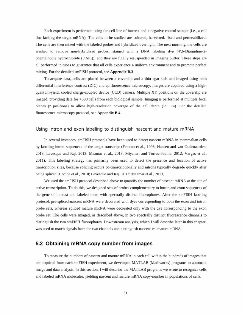
31

Each experiment is performed using the cell line of interest and a negative control sample (i.e., a cell

line lacking the target mRNA). The cells to be studied are cultured, harvested, fixed and permeabilized.

The cells are then mixed with the labeled probes and hybridized overnight. The next morning, the cells are

washed to remove non-hybridized probes, stained with a DNA labeling dye (4′,6-Diamidino-2-

phenylindole hydrochloride (DAPI)), and they are finally resuspended in imaging buffer. These steps are

all performed in tubes to guarantee that all cells experience a uniform environment and to promote perfect

mixing. For the detailed smFISH protocol, see Appendix B.3.

To acquire data, cells are placed between a coverslip and a thin agar slab and imaged using both

differential interference contrast (DIC) and epifluorescence microscopy. Images are acquired using a high-

quantum-yield, cooled charge-coupled device (CCD) camera. Multiple XY positions on the coverslip are

imaged, providing data for >300 cells from each biological sample. Imaging is performed at multiple focal

planes (z positions) to allow high-resolution coverage of the cell depth (~5 μm). For the detailed

fluorescence microscopy protocol, see Appendix B.4.

Using intron and exon labeling to distinguish nascent and mature mRNA

In several instances, smFISH protocols have been used to detect nascent mRNA in mammalian cells

by labeling intron sequences of the target transcript (Femino et al., 1998; Hansen and van Oudenaarden,

2013; Levesque and Raj, 2013; Maamar et al., 2013; Miyanari and Torres-Padilla, 2012; Vargas et al.,

2011). This labeling strategy has primarily been used to detect the presence and location of active

transcription sites, because splicing occurs co-transcriptionally and introns typically degrade quickly after

being spliced (Hocine et al., 2010; Levesque and Raj, 2013; Maamar et al., 2013).

We used the smFISH protocol described above to quantify the number of nascent mRNA at the site of

active transcription. To do this, we designed sets of probes complementary to intron and exon sequences of

the gene of interest and labeled them with spectrally distinct fluorophores. After the smFISH labeling

protocol, pre-spliced nascent mRNA were decorated with dyes corresponding to both the exon and intron

probe sets, whereas spliced mature mRNA were decorated only with the dye corresponding to the exon

probe set. The cells were imaged, as described above, in two spectrally distinct fluorescence channels to

distinguish the two smFISH fluorophores. Downstream analysis, which I will describe later in this chapter,

was used to match signals from the two channels and distinguish nascent vs. mature mRNA.

5.2 Obtaining mRNA copy number from images

To measure the numbers of nascent and mature mRNA in each cell within the hundreds of images that

are acquired from each smFISH experiment, we developed MATLAB (Mathworks) programs to automate

image and data analysis. In this section, I will describe the MATLAB programs we wrote to recognize cells

and labeled mRNA molecules, yielding nascent and mature mRNA copy-number in populations of cells.

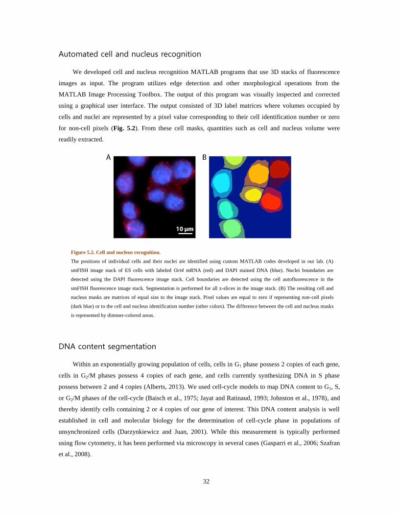
32

Automated cell and nucleus recognition

We developed cell and nucleus recognition MATLAB programs that use 3D stacks of fluorescence

images as input. The program utilizes edge detection and other morphological operations from the

MATLAB Image Processing Toolbox. The output of this program was visually inspected and corrected

using a graphical user interface. The output consisted of 3D label matrices where volumes occupied by

cells and nuclei are represented by a pixel value corresponding to their cell identification number or zero

for non-cell pixels (Fig. 5.2). From these cell masks, quantities such as cell and nucleus volume were

readily extracted.

DNA content segmentation

Within an exponentially growing population of cells, cells in G1 phase possess 2 copies of each gene,

cells in G2/M phases possess 4 copies of each gene, and cells currently synthesizing DNA in S phase

possess between 2 and 4 copies (Alberts, 2013). We used cell-cycle models to map DNA content to G1, S,

or G2/M phases of the cell-cycle (Baisch et al., 1975; Jayat and Ratinaud, 1993; Johnston et al., 1978), and

thereby identify cells containing 2 or 4 copies of our gene of interest. This DNA content analysis is well

established in cell and molecular biology for the determination of cell-cycle phase in populations of

unsynchronized cells (Darzynkiewicz and Juan, 2001). While this measurement is typically performed

using flow cytometry, it has been performed via microscopy in several cases (Gasparri et al., 2006; Szafran

et al., 2008).

Figure 5.2. Cell and nucleus recognition.

The positions of individual cells and their nuclei are identified using custom MATLAB codes developed in our lab. (A)

smFISH image stack of ES cells with labeled Oct4 mRNA (red) and DAPI stained DNA (blue). Nuclei boundaries are

detected using the DAPI fluorescence image stack. Cell boundaries are detected using the cell autofluorescence in the

smFISH fluorescence image stack. Segmentation is performed for all z-slices in the image stack. (B) The resulting cell and

nucleus masks are matrices of equal size to the image stack. Pixel values are equal to zero if representing non-cell pixels

(dark blue) or to the cell and nucleus identification number (other colors). The difference between the cell and nucleus masks

is represented by dimmer-colored areas.

33

Briefly, DNA content was quantified by integrating over the DAPI fluorescence signal within each

nucleus (defined by the 3D nucleus masks generated above). The DNA content distribution from all cells

was fit using the Fried/Baisch model (Johnston

et al., 1978), which models the DNA content

of the cells in G1 phase as a Gaussian

distribution with mean, µ, and standard

deviation, σ. The DNA of cells in G2/M phase

follows a Gaussian distribution with mean 2µ

and standard deviation 2σ, such that the

coefficient of variation (σ/µ) is equal for each

Gaussian. The DNA content of cells in S phase

is approximated by a summation of 3

Gaussians each with coefficients of variation

equal to that of G1. Therefore, the only fitting

parameters are the mean, µ, and width, σ, of

the G1 distribution, and the amplitude of each

Gaussian (Fig. 5.3A,B).

For cell-cycle stage determination, cells

are typically categorized (gated) as: G1 phase if

DNA < µ, G2/M phases if DNA > 2µ, and S

phase for all other cells. This stringent DNA

gating is preferred to avoid contamination of

G1 from cells in S phase (Johnston, 1978).

Using this method, we measured 24% in G1

phase, 65% in S phase, and 11% in G2/M

phases (357 cells), which is very similar to the

cell-cycle structure measured by flow

cytometry for mouse ES cells (18%, 63%,

19%, (Savatier et al., 1994) and 26%, 52%,

22%, (Stead et al., 2002)). Our lower

estimation of G2/M cells may be caused by

poorer performance of nucleus recognition on

cells undergoing mitosis.

We next used the fit parameters, µ and σ,

to identify cells with 2 copies and 4 copies of

our genes of interest. For Oct4 and Nanog, it is

not known when gene replication occurs,

Figure 5.3. DNA content segmentation.

(A) The DNA content histogram of ES cells (grey; 357 cells)

was fit to a prediction of a cell-cycle model (solid line). The cell

cycle model is the sum of 5 Gaussian distributions (dashed

lines). The model represents the DNA contents of cells in G1

and G2/M phases with Gaussian distributions with mean DNA

contents of µ and 2µ, respectively; the widths of these

Gaussians are σ and 2σ. The DNA contents of cells is S phase

were approximated as a summation of 3 Gaussians. (B) The fit

parameters of the cell-cycle model, µ and σ, were extracted for

use in defining DNA content gates for gene copy-number

estimation. (C) The resulting gates were used to map DNA

content to estimated gene copy-number.

34

although there is evidence that they replicate within the first half of S phase (Hiratani et al., 2008;

Schneider and Grosschedl, 2007). For the purpose of increasing the number of cells with 2 gene copies and

thereby increasing the accuracy of transcriptional kinetics estimation (Chapter 6), we gated the 2 gene-

copy cells by eye to approximately half way between µ and the beginning of the plateau feature of S cells

(Fig. 5.3B). This gate position typically corresponded to DNA ≈ µ+σ. Cells with less than this DNA value

were categorized as 2 gene-copy cells. Cells were categorized as 4 gene-copy cells if DNA > 2µ (Fig.

5.3C). We examined the effect of DNA gate position on parameter estimation and found that it was robust

to a range of gate choices (data not shown). Cells with estimated gene copy-number were grouped for use

in all subsequent analysis steps. The determined gene copy number will be of critical importance when

extracting transcription kinetics and investigating the effect of cell-cycle on transcription activity (Chapter

6).

3D spot recognition

We developed the MATLAB spot-recognition software, Spätzcells, to identify and measure the

properties of fluorescent foci (spots) across multiple focal planes in image stacks (Fig. 5.4A). The

algorithm works as follows: Spätzcells first identifies 2D local maxima of fluorescence intensity, with

height above a predefined ‘spot detection threshold’ (Fig. 5.4B). These maxima are then classified as spots

only if they appear in multiple adjacent image planes (z positions). Finally, for each spot, the fluorescence

intensity profile (at the focal plane where the spot is in focus) is fitted to a 2D Gaussian function (Fig.

5.4C), and features such as the position, peak height (amplitude of the Gaussian fit) and the integrated

fluorescence intensity are recorded. In the case that other spots are present in the vicinity of the spot being

fitted, a 2D multi-Gaussian fit is performed (see Appendix C.1 for detailed description of the algorithm).

Figure 5.4. Spot detection and quantification.

(A) smFISH image of ES cells with labeled Oct4 mRNA (red). Fluorescence image stacks are used as input in the

spot detection software, Spätzcells, developed in our lab. (B) Spätzcells first identifies spots as local maxima. (C)

Each spot is fit to a 2D Gaussian to quantify the intensity. Spots are then allocated to individual cells using the cell

masks generated previously.

35

Distinguishing real spots from false positives

Low spot detection thresholds used to recognize spots ensure that all genuine spots (i.e., spots

corresponding to target mRNA) are recognized, with the drawback of increasing the number of false

positives. Such false positives were discarded by comparing the peak height distributions of the spots in the

negative control sample to the ones in the positive sample. A ‘false-positive threshold’ was selected in peak

height that separated the population of false positives from the population of genuine spots in the positive

sample (Fig. 5.5). Spots with peak heights lower than this false-positive threshold were discarded from the

subsequent analysis of all samples.

Spot calibration and counting

A spot intensity histogram was

constructed using the remaining

spots in the positive sample. This

histogram showed a predominant

species, corresponding to a single

mRNA molecule (Fig. 5.6). The

complete histogram was fitted to a

sum of Gaussians with increasing

peak positions and decreasing peak

heights, corresponding to one, two,

three and so on mRNA molecules

per spot. Each Gaussian in this sum

has a mean that is an integer

multiple of the first Gaussian and a

variance that scales with the mean,

Figure 5.5. Discarding false positive spots.

Histogram of spot intensities quantified by

Spätzcells for the positive sample (~60,000

spots from 480 ES cells labeled with Oct4

probes, red) and the negative sample (~5,000

spots from 216 Fibroblast cells labeled with

Oct4 probes, blue). False-positive spots,

which are the result of probe binding to

nontarget RNA, are discarded after

examination of the histogram of peak height

(spot intensity maximum) in the negative

sample.

Figure 5.6. Identifying fluorescence intensity of one mRNA.

Single spot intensity histogram from Oct4 mature mRNA (~56,000 spots). The spot

intensity corresponding to a single mRNA molecule is identified by examining the

histogram of single spot intensities.

36

reflecting the statistical independence of labeling and detecting individual mRNA (Zenklusen et al., 2008).

The single-mRNA intensity was estimated as the mean of the first Gaussian. The spot fluorescence was

then converted to the number of mRNA molecules by dividing the intensity of each spot by the intensity of

the single mRNA molecule, identified as above.

Identification of nascent and mature mRNA

To identify pre-spliced nascent mRNA, which we expect to appear in both intron and exon channels,

each intron spot was matched to the closest exon spot within 200nm in x and y, and within 500nm in z

(approximately the width of the point spread function). Intron spots that were not matched with the above

criteria were not used in further analysis. Exons spots that were not matched were assumed to be mature

mRNA. The quantification of number of nascent mRNA and mature mRNA per spot was performed using

the exon probe set channel. With this strategy of using the intron channel to identify nascent mRNA and the

exon channel to quantify nascent mRNA and mature mRNA, we were able to sidestep complications of

nascent mRNA counting due to co-transcriptional spicing.

5.3 Nascent and mature mRNA copy-numbers of Oct4 and Nanog

The measured nascent and mature mRNA copy-numbers for ES cells with 2 gene copies are listed in

Table 5.1. Error represents standard error measured from three biological replicates with ~1000 cells for

each gene. A convenient way to quantify cell-to-cell heterogeneity is with the Fano Factor (Thattai and van

Oudenaarden, 2001), equal to the ratio of the square of standard deviation to the mean ( ⁄ ). We

can see from the Fano Factor of Oct4 and Nanog, that Nanog displays more cell-to-cell heterogeneity than

Oct4 at the level of mRNA.

We used mouse embryonic fibroblasts (known to not express Oct4 or Nanog) as the negative control

cell line to estimate the background of mRNA counting due to non-specific binding of probes. The mean

values of nascent and mature mRNA in fibroblasts are typically <1% of that in ES cells.

Table 5.1

Mature mRNA Nascent mRNA

Mean

( )

Standard

deviation ( )

Fano Factor

( ⁄ )

Mean

( )

Standard

deviation ( )

Fano Factor

( ⁄ )

Oct4 408±53 127±14 40±4 2.6±0.9 3.4±0.8 4.7±1.1

Nanog 104±17 78±11 59±11 2.0±0.7 3.2±0.7 5.5±0.4

37

5.4 Accuracy and dynamic range of smFISH measurements

The protocol allows measuring the absolute number of endogenous nascent and mature mRNA

molecules from a gene of interest in individual cells. The dynamic range of the measurement is from <1 to

<103 molecules per cell (Raj et al., 2006). The estimated precision of the measurement is <1 (i.e., single-

molecule resolution) at low mRNA levels (Fig. 5.6). Under the assumption that the labeling and detection

of individual mRNA molecules are statistically independent (Zenklusen et al., 2008), this translates to an

error of a few percent at the higher end of the measurement range. Although other factors may increase the

measurement error, the low error estimation is supported by the good agreement that smFISH data show

with results obtained by RNA-sequencing (RNA-seq; (Hebenstreit et al., 2011)), or with the MS2 labeling

scheme (Darzacq et al., 2007).

The presence of RNA binding proteins (such as ribosomes) could potentially affect the accessibility of

the target sequences of probes. To test for evidence of this, all spots within cells were classified as nuclear

or cytoplasmic based on the nuclear masks. Then, the distributions of intensities of nuclear and cytoplasmic

spots were compared. We found that the single spot intensity was roughly the same for both distributions,

and the nuclear spot intensity distribution contained more spots corresponding to multiple mRNA (data not

shown). From this inspection, we assume that the effects on smFISH probe binding due to the presence of

RNA binding proteins are negligible.

5.5 Limitations of smFISH

As described above, the purpose of the protocol is to obtain a precise estimate of the number of

mRNA molecules from a gene of interest in individual cells. Achieving this goal can be hindered by a

number of factors. First, the calibration of fluorescence intensity to the number of mRNA molecules

requires the use of a completely negative (i.e., no mRNA of interest present) control sample in order to

discard false-positive spots. There may be cases in which this control is not available, for example, if the

gene of interest is essential and cannot be deleted. In those cases, calibration is harder to perform and may

result in lower accuracy.

Second, we note that the accuracy of the measurement is estimated mainly using internal controls,

namely by assessing the error in identifying the single mRNA peak in the spot intensity histogram (Fig.

5.6). Additional external controls are potentially very useful. In particular, it can be helpful to compare spot

intensity with the fluorescence of individual probes in order to estimate the probe hybridization efficiency

(Trcek et al., 2012) or to compare smFISH-based mRNA levels with the results of qPCR (Klemm et al.,

2014). However, in our hands, these added measurements are more technically challenging than the

smFISH measurements themselves and are harder to render quantitative, and thus they are limited as

standards against which to compare the smFISH data.

38

5.6 Summary

In this chapter, I first described the experimental methods used to label nascent and mature mRNA

with fluorescently labeled probes. I then described the automated image analysis algorithms used to detect

and count the number of nascent and mature mRNA in individual cells and to determine the cell-cycle

phase of each cell. In the following chapter, I will describe how we use the mRNA copy-number statistics

to extract the underlying transcription kinetics.

39

6 Extracting transcription kinetics from nascent and mature mRNA copy-number distributions

In the previous chapter (Chapter 5), I described how we measured the copy-number of nascent and

mature mRNA in individual mouse embryonic stem cells using single-molecule fluorescent in situ

hybridization (smFISH). In this chapter, I will describe how we used phenomenological models of

transcription to extract transcription kinetics from the nascent and mature mRNA copy-number

distributions of Oct4 and Nanog. First, I will outline commonly used models of transcription and their

solutions for steady state mature mRNA distributions. Then, I will introduce a model that includes both

nascent and mature mRNA, and show how we can simplify this model to make use of the solutions of

commonly used models. I will then detail the methods used for extracting transcription kinetics, and discuss

the estimated parameters. Finally, I will show preliminary evidence for regulation of Oct4 and Nanog

across the cell-cycle. All results shown are mine, unless otherwise stated.

6.1 A stochastic, phenomenological model of transcription including nascent and mature RNA

Transcription is an inherently stochastic process because it involves hundreds of single-molecule

events driven by diffusion at biologically relevant temperatures (Acar et al., 2005; Maheshri and O'Shea,

2007; Munsky et al., 2012; Raj and van Oudenaarden, 2008; Sanchez and Golding, 2013). Additionally,

transcription involves many reactions of molecules with low copy-numbers in cells (e.g. 2-4 gene copies),

which invariably introduce fluctuations due to small numbers. Therefore, the mean-field approximations

used in ordinary differential equation modeling are often inappropriate, requiring the development and use

of stochastic models (Munsky et al., 2012; Raj and van Oudenaarden, 2008; Sanchez and Golding, 2013).

Many events that make up the mammalian transcription process have reaction rates that are typically

not known (Voss and Hager, 2014). Because of this, mechanistic molecular models of transcription are

largely unavailable for use in accurate measurement of transcription kinetics from acquired data. Typically,

coarse-grained phenomenological models can be used instead to describe the behavior of the system using a

small number of representative reactions and rates (Neuert et al., 2013; Sanchez et al., 2013).

Phenomenological models of transcription: Poisson and ‘bursty’ expression

The simplest model for transcription describes the production of mRNA transcripts with a single

constant rate, kINI, which represents the activity of a constitutively active gene (Fig. 6.1A). Each mRNA

transcript is then degraded at rate kD. The resulting steady-state probability distribution of mRNA per cell is

the Poisson distribution (Thattai and van Oudenaarden, 2001):

(6.1.1)

40

where is the probability of having m transcripts and λ=kINI/kD. Mature mRNA distributions that

follow Poisson statistics have been measured in some cases (Gandhi et al., 2011; Zenklusen et al., 2008).

The Poisson distribution has relatively low cell-to-cell heterogeneity, where the Fano Factor ( ) is

equal to 1 for all expression levels (Thattai and van Oudenaarden, 2001). The genes that have been

measured to follow Poisson statistics and have F=1 are considered, by interpretation through this model,

unregulated or constitutively expressed (Gandhi et al., 2011; Zenklusen et al., 2008). More commonly,

however, mRNA copy-number distributions are found to display higher cell-to-cell heterogeneity due to

intense periods of transcription activity followed by periods of quiescence, also known as ‘bursty’

transcription activity (Golding et al., 2005; Raj et al., 2006; So et al., 2011; Suter et al., 2011). This

heterogeneity is reflected in the mRNA copy-number distribution having F>1 (Faddah et al., 2013; Raj et

al., 2006; So et al., 2011; Zong et al., 2010). As can be seen in Table 5.1, this is certainly the case for Oct4

(F 40) and Nanog (F 60).

The two-state model (Peccoud and Ycart, 1995; Raj et al., 2006; Shahrezaei and Swain, 2008) (Fig.

6.1B) is a simple phenomenological model representing this scenario with the gene stochastically switching

between an ‘ON’ state, where transcription can initiate with rate kINI, and an ‘OFF’ state, where the gene is

silent. The rate of switching ‘ON’ is kON, and the rate of switching ‘OFF’ is kOFF. As before, the produced

transcripts are degraded with rate kD. Conveniently, the expected mRNA copy-number distribution has

been solved analytically (Peccoud and Ycart, 1995; Raj et al., 2006; Shahrezaei and Swain, 2008). The

steady-state probability distribution for number of mRNA per cell is given by:

(6.1.2)

where is probability of observing m transcripts, λ=kINI/kD, α=kON/kD, β=kOFF/kD, Γ(x) is the

Gamma function, and 1F1(x,y,z) is the confluent hypergeometric function of the first kind. Because this

model is phenomenological, ‘OFF’ and ‘ON’ switching may represent the combination of several processes

including chromatin reorganization, transcriptional pause-release, the binding and unbinding of

transcription factors, or other mechanisms (Balazsi et al., 2011; Sanchez et al., 2011; Voss and Hager,

Figure 6.1. Simple phenomenological models of

gene expression.

(A) Poisson expression. The simplest model for

gene expression is that the gene is stochastically

initiating transcription with constant rate kINI. The

produced mature mRNA transcripts (green) are

degraded stochastically with rate kD. (B) Bursty

expression. The gene stochastically switches

between ‘OFF’ and ‘ON’ states with rates kOFF and

kON. Transcription is stochastically initiated with

rate kINI. Mature mRNA transcripts are

stochastically degraded with rate kD.

41

2014). In the limit where the gene is always in the ‘ON’ state, kOFF<<kON (β<<α), Equation 6.1.2 reduces

to the Poisson distribution, Equation 6.1.1. Additionally, the Fano Factor ( ) can be calculated

for the two-state model:

(6.1.3)

Notice that F approaches 1 when kOFF tends to zero. Also, that F increases with decreasing kON.

Including deterministic elongation of nascent mRNA in the two-state model

The Poisson and two-state expression models are commonly used to interpret mature mRNA copy-

number distributions (Raj et al., 2006; So et al., 2011; Taniguchi et al., 2010; Zong et al., 2010). However,

our measurements also include nascent mRNA (Section 5.3). The majority of the nascent mRNA lifetime is

spent during transcript elongation, which is considered to proceed with a constant speed along the length of

the gene (Hoyle and Ish-Horowicz, 2013). The nascent mRNA transcript is then spliced, the introns are

quickly degraded, and the mature transcript is released from the transcription site (Hocine et al., 2010;

Hoyle and Ish-Horowicz, 2013; Levesque and Raj, 2013; Maamar et al., 2013). Therefore, we modify the

above two-state model to include nascent mRNA as an intermediate entity with a deterministic lifetime.

As in the standard two-state model, the gene switches between the ‘OFF’ and ‘ON’ states with rates

kOFF and kON, and transcription is initiated only in the ‘ON’ state with rate kINI. After transcription has been

initiated, the nascent transcript will elongate at constant speed, vEL, for total elongation time, τEL= vEL*lg,

Figure 6.2. A two-state phenomenological model including nascent and mature mRNA.

(A) The gene switches stochastically between ‘ON’ and ‘OFF’ states with rates kON and kOFF. When the gene is in the ‘ON’

state, transcription initiation occurs stochastically with rate kINI. After initiation, the nascent mRNA, containing exons (green)

and intron (red) regions, elongates at a deterministic speed, vEL, for the entirety of the gene. After elongation of the entire

gene is complete, the nascent mRNA is eliminated and converted into mature mRNA. The mature mRNA will stochastically

degrade with rate kD. (B) The model can be simplified by conversion into two separate processes with equal gene state

switching and transcription initiation kinetics.

42

where lg is the length of the gene. After elongation has proceeded to the end of the gene, the nascent mRNA

will be spliced, resulting in the maturation of the nascent mRNA into the mature mRNA transcript. Mature

mRNA transcripts are then degraded stochastically with rate kD (Fig. 6.2A). We note that there could be

further refinement of this model, including position of intron within the gene and delay between splicing

and detachment. However, we consider the model above for simplicity and to limit over-fitting the data.

Nascent and mature mRNA production can be modeled as two processes with

equal initiation kinetics

Unlike the Poisson and two-state models presented before, we are not aware of analytical solutions for

the two-state model including nascent mRNA (Fig. 6.2A). However, the two-state model including nascent

mRNA was simplified by noticing that the deterministic lifetime of nascent mRNA represents only a

deterministic ‘time delay’ before conversion into mature mRNA. Because the delay is deterministic, it

provides no added stochasticity to the distribution of mature mRNA. Therefore, nascent and mature mRNA

distributions were modeled separately assuming they share equal ‘ON’/’OFF’ switching and transcription

initiation kinetics (Fig. 6.2B).

The distributions of mature mRNA follow the standard analytical form of the two-state model with

fitting parameters, kINI/kD, kON/kD, and kOFF/kD (Peccoud and Ycart, 1995; Raj et al., 2006; Shahrezaei and

Swain, 2008). The nascent mRNA distributions were numerically calculated using a modified version (see

Appendix C.2 for detailed description) of the Finite State Projection algorithm (Munsky and Khammash,

2006; Neuert et al., 2013). The fitting parameters of this model are kINI*τEL, kON*τEL, and kOFF*τEL. When

fitting nascent and mature mRNA histograms, we constrained kINI, kON, and kOFF to be equal. Therefore, the

fitting parameters for the model of nascent and mature mRNA model were kINI*τEL, kON*τEL, kOFF*τEL, and

kD*τEL.

6.2 Modeling multiple alleles

To extract kinetic parameters, we used the subpopulation of cells that were determined to have two

gene copies (outlined in Section 5.2). However, the model including nascent and mature mRNA (Fig.

6.2B) describes mRNA produced from a single gene-copy. Therefore, we first must determine how gene

activity scales with gene copy-number to accurately extract the transcription kinetics from individual genes.

The effect of multiple copies on gene expression is not documented for the Oct4 and Nanog genes; the

genes may be regulated by non-trivial dosage effects (Torres-Padilla and Chambers, 2014). Therefore,

before we construct a transcription model containing multiple gene copies, we must first verify that the

activity from the two alleles of each gene is uncorrelated (transcriptionally independent).

To test for correlated allele activity, we measured the number of active transcription sites per cell

within the two gene-copy cells. We then calculated the Pearson correlation coefficient, ( ⟨ ⟩

),

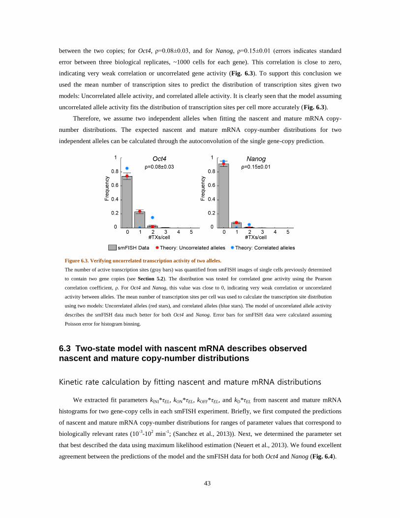
43

between the two copies; for Oct4, ρ=0.08±0.03, and for Nanog, ρ=0.15±0.01 (errors indicates standard

error between three biological replicates, ~1000 cells for each gene). This correlation is close to zero,

indicating very weak correlation or uncorrelated gene activity (Fig. 6.3). To support this conclusion we

used the mean number of transcription sites to predict the distribution of transcription sites given two

models: Uncorrelated allele activity, and correlated allele activity. It is clearly seen that the model assuming

uncorrelated allele activity fits the distribution of transcription sites per cell more accurately (Fig. 6.3).

Therefore, we assume two independent alleles when fitting the nascent and mature mRNA copy-

number distributions. The expected nascent and mature mRNA copy-number distributions for two

independent alleles can be calculated through the autoconvolution of the single gene-copy prediction.

6.3 Two-state model with nascent mRNA describes observed nascent and mature copy-number distributions

Kinetic rate calculation by fitting nascent and mature mRNA distributions

We extracted fit parameters kINI*τEL, kON*τEL, kOFF*τEL, and kD*τEL from nascent and mature mRNA

histograms for two gene-copy cells in each smFISH experiment. Briefly, we first computed the predictions

of nascent and mature mRNA copy-number distributions for ranges of parameter values that correspond to

biologically relevant rates (10-3

-102 min

-1; (Sanchez et al., 2013)). Next, we determined the parameter set

that best described the data using maximum likelihood estimation (Neuert et al., 2013). We found excellent

agreement between the predictions of the model and the smFISH data for both Oct4 and Nanog (Fig. 6.4).

Figure 6.3. Verifying uncorrelated transcription activity of two alleles.

The number of active transcription sites (gray bars) was quantified from smFISH images of single cells previously determined

to contain two gene copies (see Section 5.2). The distribution was tested for correlated gene activity using the Pearson

correlation coefficient, ρ. For Oct4 and Nanog, this value was close to 0, indicating very weak correlation or uncorrelated

activity between alleles. The mean number of transcription sites per cell was used to calculate the transcription site distribution

using two models: Uncorrelated alleles (red stars), and correlated alleles (blue stars). The model of uncorrelated allele activity

describes the smFISH data much better for both Oct4 and Nanog. Error bars for smFISH data were calculated assuming

Poisson error for histogram binning.

44

To calculate the rates, kON, kOFF, kINI and kD, we first estimated the elongation time for each gene

according to the formula τEL= vEL*lg. The polymerase elongation speed, vEL=2.8 kb/min was taken from the

literature (Ardehali and Lis, 2009). The length of the genes are known (lg,Oct4=4.7bp, lg,Nanog=7.1bp). The

rates kON, kOFF, kINI and kD, were then calculated by dividing the fit parameters by the elongation time.

Table 6.1 shows the calculated rates and elongation speeds for Oct4 and Nanog. The error in calculated

rates indicates the standard error from 3 biological replicates with ~1000 cells for each gene.

Table 6.1

kON (min-1

) kOFF (min-1

) kINI (min-1

) kD (min-1

) τEL (min)

Oct4 1.9x10-2±4.4x10-3 3.2x10-2±7.8x10-3 3.7±8.7x10-1 6.9x10-3±1.0x10-3 1.7

Nanog 6.3x10-3±2.4x10-3 2.7x10-2±5.0x10-3 2.5±5.2x10-1 7.9x10-3±2.6x10-3 2.5

Figure 6.4. Two-state model accurately fits smFISH distributions of mature and nascent mRNA.

The number of mature and nascent mRNA distributions quantified using smFISH from individual cells

(grey bars) were fit simultaneously to the two-state model including nascent mRNA (red lines). The fit

was able to capture the shape of the distributions very well.

45

Comparison of kinetic rates between Oct4 and Nanog

As reflected in the Fano Factor (Table 5.1), Oct4 and Nanog displayed nascent and mature mRNA

heterogeneity which indicated some form of regulated gene expression (Munsky et al., 2012; Sanchez and

Golding, 2013). The nascent and mature mRNA distributions were fit to the two-state model and the kinetic

rates of the model were measured for Oct4 and

Nanog (Table 6.1). Surprisingly, for both

genes studied, all of the measured rates were

approximately equal except for kON. Therefore,

using the interpretation given by the two-state

model, the relatively large mRNA

heterogeneity of Nanog relative to Oct4 is a

manifestation of Nanog having a lower rate of

turning ‘ON’ relative to Oct4 (Fig. 6.5).

As described above (Section 6.1), the

kinetic steps in the two-state

phenomenological model may represent many

different underlying mechanisms. The loci of

Nanog and Oct4 are known to be regulated by

many different factors (Young, 2011).

However, the observation that only kON was

different between the two genes may

potentially direct further studies.

6.4 Analysis of dosage compensation across the cell cycle

Gene activity for Oct4 and Nanog does not double after gene replication

To investigate if the cell cycle affects Oct4 or Nanog gene expression, we first compared the mean

number per cell of mature mRNA, nascent mRNA, and active transcription sites between cells that have

two gene-copies and cells that have four gene-copies (determined in Section 5.2). As a control for the

measurement of gene expression change after gene replication, we used a mouse ES cell line that contains a

single-copy of lacZ under a highly expressed constitutive viral promoter (Z/Red, (Vintersten et al., 2004))

which is not believed to be regulated by the cell-cycle.

We found that the mean number per cell of mature mRNA, nascent mRNA, and active transcription

sites increased after gene replication for all genes. Because the numbers of nascent mRNA and active

transcription sites were expected to scale linearly with gene copy-number, we expected to observe a two-

fold increase after gene replication. For lacZ nascent mRNA and transcription sites, the increase after gene

Figure 6.5. Extracted kinetics of transcription for Oct4 and Nanog.

The two-state model including nascent mRNA was fit to the

distributions of nascent and mature mRNA from smFISH data. The best

fit parameters were extracted and converted into kinetic rates. The

primary difference between Oct4 and Nanog is in the kON rate, where

kON of Nanog is ~3-fold lower than that of Oct4.

46

replication was approximately two fold. However, for Oct4 and Nanog, the observed increase was

significantly less than twofold (Fig. 6.6). Additionally, the number of nascent mRNA at each transcription

site remained the same before and after gene replication.

We interpreted these data as supporting dosage compensation of Oct4 and Nanog. We have already

shown that the observed gene activity of Oct4 and Nanog is consistent with bursty gene expression

(Section 6.3). Under this framework, these data suggest that the frequency of an allele becoming active, or

Figure 6.6. Preliminary evidence of dosage compensation in Oct4 and Nanog.

Left columns represent the mean number of observables per cell measured in smFISH experiments before gene

replication (light grey bars) and after gene replication (dark grey bars). Right column represents the fold change

observed from before to after gene replication. (A) Mature mRNA (B) Nascent mRNA (C) Transcription sites (D)

Nascent mRNA at transcription sites. Notice that LacZ exhibits a 2-fold increase from before to after gene replication

for nascent mRNA and for number of transcription sites as expected after gene replication, whereas Oct4 and Nanog

exhibit lower that 2-fold increase in nascent mRNA and transcription sites, suggesting dosage compensation. All genes

do not exhibit any difference in number of nascent mRNA at the gene from before to after gene replication.

47

transcriptionally bursting, decreases after gene replication, whereas the number of nascent mRNA produced

from each transcription burst remains constant. This is potentially another mode of transcriptional

regulation that could modify the cell-to-cell mRNA copy-number variability.

This kinetic interpretation would be better demonstrated with support from the fit to two-state models

that was performed in Section 6.3. However, additional experiments would be needed as the number of

cells with four gene copies is too few for accurate mRNA distribution fitting.

6.5 Summary

In this chapter, I used a phenomenological two-state model to measure transcription kinetics of Oct4

and Nanog from the smFISH data acquired previously (Chapter 5). Both Oct4 and Nanog exhibited

nascent and mature mRNA distributions that were well described by the two-state model. Through this

two-state model, we demonstrated that the source of mRNA heterogeneity displayed in Nanog compared to

Oct4 can be reduced to a slower rate at which Nanog turns ‘ON’ compared to Oct4. Additionally, we found

evidence supporting dosage compensation of Oct4 and Nanog.

48

Glossary

Allele – One of several alternate forms of a gene. In a diploid cell each gene will have two alleles.

Asymmetric cell division – Division producing two daughter cells with different cell fates.

Cell cycle – Reproductive cycle of a cell: the sequence of events by which a cell duplicates its

chromosomes and divides in two daughter cells. For eukaryotic cells: G1 (cell size increase and

checkpoint before DNA synthesis), S (DNA synthesis), G2 (cell size increase and checkpoint

before mitosis), M (mitosis).

Chromatin – Complex of DNA and histones (DNA binding proteins) condenses DNA.

Cytokine – Cellular signaling protein that acts as a mediator in cell-cell communication.

Differentiation – Process by which a cell undergoes changes into a specialized cell type.

Embryogenesis – The process by which an embryo develops.

Enhancer – Regulatory DNA sequence to which proteins bind, increasing the rate of transcription of a

gene. The enhancer can be thousands of basepairs away from the gene.

Excitable system – A system that has: a unique attracting state, and enough stimulus to send through

long excursions through state space.

Exon – Segment of a gene that will be represented in the mature mRNA.

Fibroblast – Common cell type found in connective tissue. Secretes proteins that act as differentiation

inhibitors for ES cells.

Gene regulatory network – A network of genes that regulate each other indirectly through RNA,

protein, or other signaling molecules.

Intron – Noncoding region of DNA that is transcribed into nascent RNA, but is excised during

splicing.

Leukemia inhibitory factor (LIF) – A cytokine that affects cell growth and prevents differentiation.

During early embryo development, LIF is supplied to inner cell mass cells by the trophectoderm.

In vitro culturing methods involve supplementing LIF into growth media.

Mature mRNA – RNA molecule that specifies the amino acid sequence of a protein.

MicroRNA – RNA molecules ~20 nucleotides in length that regulate gene expression through

complementary base-paring with mRNA.

Mitosis – Division of the nucleus involving condensation of DNA into chromosomes and then

segregating chromosomes equally to each daughter cell.

Nascent mRNA – Recently produced mRNA. Contains intron and exon sequences before being

spliced.

Plaque – A visible hole (~1 mm in diameter) in a bacterial lawn due to multiple rounds of

bacteriophage infection and lysis.

Promoter – DNA sequence to which RNA polymerase binds. Can include DNA regulatory elements

that increase or decrease transcription via proteins or small molecules.

49

Prophage – Integrated bacteriophage genome in bacterial chromosome.

RNA polymerase – Enzyme that produces nascent RNA using DNA sequences as a template.

Splicing – Removal of intron sequences from nascent RNA transcripts by concatenating exons on

either side of each intron.

Symmetric cell division – Division producing two daughter cells with the same cell fates.

Titering phage stock – Measuring concentration of viable phage particles in a solution (typically

measured in plaque forming units per milliliter).

Transcription – Copying one strand of DNA into a complementary sequence of RNA by RNA

polymerase.

Transcription factor – Protein or molecule that regulates transcription (e.g. recruiting RNA

polymerase, chromatin remodeling).

50

Appendix A. Bacteriophage lambda experimental protocols

A.1 Strains, growth media and growth conditions

Media and growth conditions

All strains were grown in Luria-Bertani Lennox (LB) media unless otherwise stated. 1 liter of LB

broth includes: 5 g sodium chloride (Fisher Scientific, #BP358-1), 10 g tryptone (BD, #211705), 5 g yeast

extract (BD, #212750), pH 7.0 adjusted with 1M NaOH (Fisher Scientific, #BP359-500). LB was sterilized

by autoclaving.

Media supplements used in bacteriophage lambda protocols commonly include: 10 mM MgSO4

(autoclaved) (Fisher Scientific, #BP213-1) to stabilize phage capsids, 0.2% maltose (filter-sterilized)

(Fisher Scientific, #BP684-500) to repress expression of LamB maltose uptake receptors, 0.2% glucose

(filter-sterilized) (Fisher Scientific, #BP350-500) to repress expression of LamB maltose uptake receptors.

Optical density of cell culture was measured using Bio-Rad SmartSpec Plus.

Bacterial strains

Bacterial strains used in this work are listed in Table A.1.

Table A.1

Strain Relevant genotype Reference Source

MG1655 Wildtype Lab Stock

LE392 supF John Cronan

C600 sup0 Appleyard, 1954 Lab Stock

JL5902 RecA+ Little, Shepley et al., 1999 John Little

JL2497 RecA-

Little, Shepley et al., 1999 John Little

NC416 luc-N’…cro+ cII’-lacZYA Svenningsten, Constantino et al. 2005 Donald Court

51

Bacteriophage lambda strains

Phage strains used in this work are listed in Table A.2.

Table A.2

Strain Relevant genotype Reference Source

ʎIG831 bor::kanR Lab stock

ʎIG2903 cI857 bor::kanR Lab stock

ʎeyfp cI857 Sam7 D-eyfp Alvarez et al., 2007 Phillippe Thomen

ʎLZ1 cI857 Sam7 D-eyfp b::kanR Lab stock

ʎsus123 Dam123 Campbell, 1961 Allan Campbell

ʎsus15 Dam15 Campbell, 1961 Michael Feiss

ʎSOS2 D-eyfp b::kanR Lab stock

ʎIG2504 cIT88C Saur, Jordan et al., 1990 Lab stock

ʎIG28061 cIV361 Lim and Sauer, 1989 Lab stock

ʎIG04061 cI E34K

GAA-AAA

Saur, Jordan et al., 1990 Lab stock

ʎIG28062 cIL18V Lim and Sauer, 1989 Lab stock

ʎJL815 cID38N Michalowski and Little, 2005 John Little

ʎNP2 cI D38N

PRM-35 TAGA-GCTG

PRM-10 GATT-TATT

Michalowski and Little, 2005 John Little

ʎNP3 cI D38N

PRM-35 TAGA-CATT

PRM-10 GATT-GAAT

Michalowski and Little, 2005 John Little

ʎNP4 cI D38N

PRM-35 TAGA-CCTT

PRM-10 GATT-CCAT

Michalowski and Little, 2005 John Little

ʎNP5 cI D38N

PRM-35 TAGA-CTAA

PRM-10 GATT-GAAT

Michalowski and Little, 2005 John Little

ʎNP6 cI D38N

PRM-35 TAGA-CCCA

PRM-10 GATT-TGAT

Michalowski and Little, 2005 John Little

ʎNP7 cI D38N

PRM-35 TAGA-TACC

PRM-10 GATT-TACT

Michalowski and Little, 2005 John Little

52

ʎNP8 cI D38N

PRM-35 TAGA-GTGT

PRM-10 GATT-GTAT

Michalowski and Little, 2005 John Little

ʎNP10 cI D38N

PRM-35 TAGA-CCAA

PRM-10 GATT-GAAT

Michalowski and Little, 2005 John Little

ʎNP11 cI D38N

PRM-35 TAGA-CTCA

PRM-10 GATT-TGCT

Michalowski and Little, 2005 John Little

53

A.2 Bacteriophage propagation and handling

These procedures constitute basic phage propagation: the revival of stable long-term stocks,

maintaining liquid phage stocks of high concentration, and the creation of a downstream long-term stock.

Phage strains are most stable for long-term storage in the form of a prophage in lysogen cells (if lysogen

pathway is not compromised). Long-term stocks of lysogens are frozen in media + 15% glycerol (Fisher

Scientific, #BP229-1) and stored at -80°C. If stored as a prophage, obtaining a phage lysate requires

lysogen induction. The phage concentration of the lysate is estimated by titration of plaque forming units

per milliliter (pfu/ml). A phage stock that has decreased in pfu/ml can be plate-amplified, a process to make

a large, stable quantity of high-titer phage stock. The phage stock can be used to make lysogens by

infecting other host strains for long-term storage.

Sterile, aerosol-barrier pipette tips were used in all protocols.

Titering phage concentration

An overnight culture of indicator strain was grown in LB+0.2% maltose and 10mM MgSO4 (LBMM)

at 37°C. Cells were diluted 1:100 in LBMM and grown at 37°C to OD600≈0.4. The cells were centrifuged at

1000g for 10 min at 4°C and the pellet was gently resuspended in one tenth of the original volume in

phosphate buffered saline (PBS; Fisher Scientific, #BP24384)+10 mM MgSO4. The indicator strains can be

stored at 4°C for 24 hours.

The phage stock to be titered was diluted in SM buffer (Teknova, #S0249) to an estimated 104 pfu/ml

to give ≈100 plaques/plate. 100 µl of cells were mixed with 10 µl of phage dilution and incubated at 37°C

for 15 min to provide optimal conditions for phage adsorption on the cells. The phage-cell mixture was

then added into 3 ml of 48°C molten NZYM (Teknova, #N2062) top agar, and plated immediately on dry,

pre-warmed NZYM agar plates. The plates were allowed to set for 10 min, then inverted and incubated for

12–16 hr at 37°C. The titer in pfu/ml was then determined by counting the plaques and multiplying by the

dilution factor.

Mitomycin-C induction of wildtype prophages

An overnight lysogen culture was grown in LB supplemented with the appropriate antibiotics at 37°C.

Cells were diluted 1:100 into 10 ml LB+0.2% glucose and 10mM MgSO4 (LBGM) and grown at 37°C with

gentle shaking (180 rpm) to OD600≈0.4. The culture was induced by adding Mitomycin-C (Sigma, #M4287)

to 10 µg/ml final concentration. The culture was incubated at 37°C until lysis was visible. Chloroform

(Fisher Scientific, #C298-500) was added to 2% (v/v) final concentration. The lysate was mixed gently by

hand and incubated for 15 min at room temperature. The lysate was then decanted into a 15 ml centrifuge

tube and centrifuged at 3500g for 10 min at 4°C. The supernatant was transferred to a new 15 ml centrifuge

tube and checked for remaining cell debris. If cell debris was visible, 2% chloroform was added and

54

centrifuged as before. If no cell debris was visible, chloroform was added to 0.3% (v/v) final concentration

for storage. The phage stock was then stored at 4°C and phage concentration was titered periodically.

Heat induction of temperature-sensitive prophages (cI857)

An overnight lysogen culture was grown in LB supplemented with the appropriate antibiotic at 30°C.

Cells were diluted 1:100 into 15 ml of LB+0.2% glucose and 10mM MgSO4 (LBGM) and grown at 30°C

with gentle shaking (180 rpm) to OD600≈0.4. The culture was induced at 42°C with gentle shaking (180

rpm) for 15 min and then was incubated at 37°C with gentle shaking until lysis was visible (~90 min after

induction). Chloroform (Fisher Scientific, #C298-500) was added to 2% (v/v) final concentration. The

lysate was mixed gently by hand and incubated for 15 min at room temperature. The lysate was then

decanted into a 15 ml centrifuge tube and centrifuged at 3500g for 10 min at 4°C. The supernatant was

transferred to a new 15 ml centrifuge tube and checked for remaining cell debris. If cell debris was visible,

2% chloroform was added and centrifuged as before. If no cell debris was visible, chloroform was added to

0.3% (v/v) final concentration for storage. The phage stock was then stored at 4°C and phage concentration

was titered periodically.

Plate-amplification

An overnight culture of indicator strain was grown in LB+0.2% maltose and 10mM MgSO4 (LBMM)

at 37°C. Cells were diluted 1:100 in LBMM and grown at 37°C to OD600≈0.4. The cells were centrifuged at

1000g for 10 min at 4°C and the pellet was gently resuspended in one tenth of the original volume in

phosphate buffered saline (PBS; Fisher Scientific, #BP24384)+10 mM MgSO4. The indicator strains can be

stored at 4°C for 24 hours.

The phage stock to be amplified was diluted in SM buffer (Teknova, #S0249) to an estimated 2x106

pfu/ml to give ≈2x104 plaques/plate. 100 µl of cells were mixed with 10 µl of phage dilution and incubated

at 37°C for 15 min to provide optimal conditions for phage adsorption on the cells. The phage-cell mixture

was then added into 3 ml of 48°C molten NZYM (Teknova, #N2062) top agar, and plated immediately on

fresh thickly-poured NZYM agar plates. The plates were allowed to set for 10 min, then inverted and

incubated for 6–8 hr at 37°C. The plates were removed from the incubator before the plaque size reached

2mm (at this point, most plaques were touching). 4 ml of SM buffer was gently pipetted onto the plaque

surface. The plate was stored at 4°C for 12-16 to allow phages to diffuse into the SM buffer.

The next day, the SM buffer containing phages was gently transferred to a 15 ml centrifuge tube. The

plate was gently washed with an additional 1 ml of SM buffer and pooled. Chloroform (Fisher Scientific,

#C298-500) was added to 5% (v/v) final concentration and the phage stock was gently mixed and incubated

at room temperature for 15 min. The cell debris was removed by centrifugation for 10 min at 3500g at 4°C.

The supernatant was transferred to a new 15 ml centrifuge tube and checked for remaining cell debris. If

cell debris was visible, 5% chloroform was added and centrifuged as before. If no cell debris was visible,

55

chloroform was added to 0.3% (v/v) final concentration for storage. The phage stock was then stored at 4°C

and phage concentration was titered periodically.

Lysogenization

An overnight culture of host cells was grown in LB+0.2% maltose and 10mM MgSO4 (LBMM) at

37°C. Cells were diluted 1:100 into LBMM and grown at 37°C to OD600≈0.4. The cells were centrifuged at

1000g for 10 min at 4°C and the pellet was gently resuspended in one tenth of the original volume in fresh

LBMM at room temperature, resulting in cell concentration of ~2.5*109 cells/ml. Cells were infected at

MOI=3 (multiplicity of infection) for 20 minutes at room temperature. The infection is diluted 1:100 into

prewarmed LB+0.2% glucose and 10mM MgSO4 (LBGM) and incubated at 37°C for 30 min, allowing

successfully integrated prophages to express antibiotic resistance. Aliquots in phosphate buffered saline

(PBS; Fisher Scientific, #BP24384) were diluted and plated on LB plates containing the appropriate

antibiotic and incubated 12-16 hours at 37°C. Antibiotic resistant colonies were picked and re-streaked on

antibiotic plates.

Note: This lysogenization protocols presumes that the phage contains an antibiotic resistance cassette

in the genome for selection of lysogen cells. Lysogenization of temperature sensitive phages requires the

following modifications to the incubation conditions of the protocol: The infection is diluted 1:100 into

prewarmed LBGM and incubated at 30°C for 45 min. Aliquots in PBS are plated on LB plates containing

antibiotics and incubated at 30°C for 12-16 hours.

56

A.3 Quantitative bulk measurements

Lysogenization frequency

The lysogenization probability was measured as a function of MOI (multiplicity of infection). An

overnight of host cells was grown in LB+0.2% maltose and 10mM MgSO4 (LBMM) at 37°C. Cells were

diluted 1:100 into LBMM and grown at 37°C to OD600≈0.4. The cells were centrifuged at 1000g for 10 min

at 4°C and the pellet was gently resuspended in one tenth of the original volume in fresh LBMM at room

temperature. Cells were infected at different MOIs (from 10-5

to 102) for 20 min at room temperature,

diluted 1:100 into 1 ml prewarmed LB+0.2% glucose and 10mM MgSO4 (LBGM) and incubated at 37°C

for 30 min, allowing successfully integrated prophages to express antibiotic resistance. Aliquots in

phosphate buffered saline (PBS; Fisher Scientific, #BP24384) were plated on LB plates containing

appropriate antibiotics, and incubated 12–16 hours at 37°C. Lysogen concentrations were determined by

counting the number of antibiotic resistant colonies and multiplying that number by the dilution factor. Pre-

infection phage and bacteria concentrations were measured using standard plate assays.

The lysogenization probability was plotted as a function of MOI on a log-log scale. Wildtype phages

will produce a line with a slope of ~2 indicating the requirement for infection by at least 2 phages for

lysogeny (See Fig. 2.1).

Note: This lysogenization protocols presumes that the phage contains an antibiotic resistance cassette

in the genome for selection of lysogen cells. Lysogenization of temperature sensitive phages requires the

following modifications to the incubation temperatures of the protocol: The infection is diluted 1:100 into

prewarmed LBGM and incubated at 30°C for 45 min. Aliquots in PBS are plated on LB plates containing

antibiotics and incubated at 30°C for 12-16 hours.

Lysogen spontaneous induction rate

An overnight lysogen culture was grown in LB+0.2% glucose and 10mM MgSO4 (LBGM)

supplemented with the appropriate antibiotic at 30°C. The overnight culture was centrifuged and

resuspended in 1 ml LBGM to discard free phages in the overnight. The washed culture was diluted 1:1000

into 15 ml LBGM and grown at the desired temperature (between 28°C and 37°C). During exponential

growth phase (OD600≈0.1–0.5), 1 ml culture was taken and OD600 value was immediately measured. 750

µl of the sample was transferred to a 1.5 ml microcentrifuge tube. Cells were lysed with the addition of 15

µl of chloroform (Fisher Scientific, #C298-500) and gentle mixing by inverting 10 times. The samples were

then stored at 4°C until measurement of the phage concentration ϕ with a standard phage titering protocol

(see Appendix A.2).

57

The number of bacterial cells, B, was estimated based on OD600 value. The average number of phages

released per lysis, M, was measured separately, as described in the next section. The spontaneous induction

rate was calculated based on the formula (see Appendix D.1 for detailed derivation).

“One-step” burst size measurement

An overnight culture of cells was grown in LB+0.2% maltose and 10mM MgSO4 (LBMM) at 37°C.

An overday culture of indicator cells was made by diluting the overnight culture 1:10 into LBMM and

grown at 37°C to saturation at OD600≈4. The indicator cells were centrifuged at 1000g for 10 min at 4°C

and the pellet was gently resuspended in one tenth of the original volume in LBMM and leave at room

temperature.

An overday culture of host cells was made by diluting the overnight culture 1:100 into 10 ml LBMM

and grown at 37°C to OD600≈0.4. The cells were centrifuged at 1000g for 10 min at 4°C and the pellet was

gently resuspended in one tenth of the original volume in fresh LBMM at room temperature. Cells were

infected at MOI=0.1 for 20 min at room temperature, diluted 1:104 into 10 ml prewarmed LB+0.2%

glucose and 10mM MgSO4 (LBGM) and incubated at 37°C. At time points (~10 min) after dilution, 100 µl

aliquots were taken and serially diluted in SM buffer (Teknova, #S0249). 10 µl of phage dilution and 100

µl of dense indicator cell stock were added to 3 ml of 48°C molten NZYM (Teknova, #N2062) top agar and

plated immediately on dry, pre-warmed NZYM agar plates. The plates were allowed to set for 10 min, then

inverted and incubated for 12–16 hr at 37°C. The titer in pfu/ml was then determined by counting the

plaques and multiplying by the dilution factor.

58

A.4 Genetic manipulation

Crossing D-eyfp from a plasmid onto a ʎ-Dam phage

A gpD-eyfp phage, ʎLZ1, was obtained by crossing ʎeyfp [cI857 Sam7 D-eyfp] (gift of Phillippe

Thomen, Universite Pierre at Marie Curie) with plasmid pJWL464 (gift of John Little, University of

Arizona), resulting in a kanR cassette inserted into ʎ b region, which is considered nonessential. We

observed that ʎLZ1 had several phenotypic differences with wildtype ʎ. To test the hypothesis that D-eyfp

was not the source of these phenotypic differences, we aimed to engineer a gpD-eyfp, but otherwise

wildtype, phage. To accomplish this, D-eyfp was crossed onto ʎsus123 [Dam123] (gift of Allan Campbell,

University of Rochester), where D-eyfp replaced the amber mutated D during this recombination.

Briefly, D-eyfp was PCR amplified using λLZ1 as a template. Primers were designed to amplify

~650bp regions surrounding D-eyfp that were homologous to wildtype lambda. This PCR product was

ligated into plasmid pBS(+) and transformed into E. coli strain, LE392. Homologous recombination was

used to integrate this PCR product into another phage. For the purpose of efficient screening of the

recombination events, we used ʎsus123 [Dam123] (gift of Allan Campbell, University of Rochester) as the

target phage. When expressed in E. coli strain C600 (wildtype), the amber mutation in capsid protein gpD

will create non-functional gpD proteins thereby producing non-viable progeny phages. When expressed in

amber suppressor strain, LE392 [supF], the amber mutation in D is suppressed and viable progeny phages

are produced. The homologous recombination was performed by infecting LE392 containing the plasmid

with ʎsus123 and collecting the lysate. This lysate contained progeny phages resulting from successful and

unsuccessful homologous recombination events.

To select for the successful crosses, the non-permissive host, C600, was infected with a volume of

crude lysate containing ~105 pfu and plated following the standard phage titering protocol. 15 out of ~100

plaques fluoresced when viewed under a fluorescence dissecting microscope (Zeiss). 4 fluorescent plaques

were picked, incubated in SM buffer, plate amplified, and tested for uniform fluorescent-plaque generation.

ʎSOS2 was created by crossing one fluorescent phage stock with plasmid pJWL464, resulting in the insertion

of a kanR cassette into ʎ b region.

59

A.5 Transmission electron microscopy

We imaged the phage under a transmission electron microscope (TEM) to examine phage morphology

(Edgar et al., 2008). 5 µl of purified phage were applied to a carbon-coated specimen grid (200-mesh Holey

carbon-coated copper grids, SPI no. 3620C). After 5 min, excess fluid was wicked away by using

Kimwipes paper to touch the edge of the grid. Five µl of negative stain, Nano-W (http://nanoprobes.com,

catalog no. 2018), were then applied to the grid. After 5 min, excess stain was wicked away in the same

way and the grid was allowed to air dry for 2 min. Specimens were then examined on a JEOL 2100 Cryo

TEM operating at 200 kV and images were recorded on a Gatan matScan1kx1k progressive scan CCD

camera.

60

Appendix B. Mouse embryonic stem cells experimental protocols

B.1 Mouse embryonic stem cell lines and media

Cell lines

Mouse cell lines used in this work are listed in Table B.1.

Table B.1

Cell line Relevant genotype Reference Source

R1 Oct4+/+, Nanog +/+ Thomas Zwaka

Z/Red Oct4+/+, Nanog +/+, LacZ Vintersten et al. 2004 Thomas Zwaka

NIH-3T3 Oct4 and Nanog not expressed Thomas Zwaka

Media and cell culture

ES and Z/Red cells were cultured in Dulbecco’s Modified Eagle’s High Glucose GlutaMAX Pyruvate

Medium (GIBCO, #10569) supplemented with 10% fetal bovine serum (FBS; GIBCO), L-Glutamine

(GIBCO), 100 nM nonessential amino acids (GIBCO), 100 mM beta-mercaptoethanol (Fluka), and 1000

U/ml LIF (Chemicon). Cells were grown on 0.1% gelatin coated dishes. Media was replaced daily. Cells

require 1:6 dilution for passaging every two days.

NIH-3T3 cells were cultured in Dulbecco’s Modified Eagle’s, high glucose Medium (GIBCO,

#11965) supplemented with 10% fetal bovine serum (FBS; GIBCO), and 1 mM sodium pyruvate (GIBCO,

#11360). Media was replaced every two days. Cells require 1:4 dilution for passaging every four days.

Storage media for all cells consisted of: 40% growth media, 50% FBS (GIBCO), and 5% Dimethyl

Sulfoxide (DMSO; Fisher Scientific #BP231-100).

61

B.2 Mammalian cell culture

Reviving frozen stocks

For ES and Z/Red cells: 1 vial of liquid nitrogen stock was revived in 1 well of a 6-well plate. 0.1%

gelatin coated 6-well culture plates were prepared by adding 2 ml of 0.1% gelatin into each well, and

incubating the plate at 37°C for 20 min. The gelatin was aspirated immediately before use. Contents from 1

vial of liquid nitrogen stock (1 ml) was thawed at 37°C (~3 min) and immediately diluted into 9 ml of fresh

media. Cells were centrifuged at 1200 rpm for 5 min and the supernatant was aspirated. The pellet was

resuspended gently in 3 ml media by pipetting up and down 10 times. Cells were then transferred to a

single well in a 0.1% gelatin coated 6-well culture plate. Cells were incubated at 37°C with 5% CO2.

For NIH-3T3 cells: 1 vial of liquid nitrogen stock was revived on a 10 cm plate. Contents from 1 vial

of liquid nitrogen stock (1 ml) was thawed at 37°C (~3 min) and immediately diluted into 9 ml of fresh

media. Cells were centrifuged at 1200 rpm for 5 min and the supernatant was aspirated. The pellet was

resuspended gently in 10 ml media by pipetting up and down 10 times and then transferred to a 10cm plate.

Cells were incubated at 37°C with 5% CO2.

Passaging

The following protocols give the example of passaging a 10 cm culture dish. Appropriate volumes of

reagents for other culture dishes are given in Table B.2.

For ES and Z/Red cells: A new 0.1% gelatin coated 10 cm culture dish was prepared by: adding 10 ml

of 0.1% gelatin, incubating the dish at 37°C for 20 min, aspirating the gelatin, and adding 8 ml of media to

the culture dish. The growth media was aspirated away from the culture dish containing confluent cells.

The cells were washed twice with 5 ml PBS by gently pipetting PBS onto the dish and aspirating. 3 ml of

prewarmed 0.05% trypsin (Gibco, #25300-054) was added to dish to cover cells. The culture dish was

incubated at 37°C for 5 min to allow for trypsin protease activity to create single cell suspension. 7 ml of

media was added to the culture dish to allow serum to deactivate trypsin. The 10 ml of cell suspension was

gently pipetted up and down 10 times and transferred to a 15 ml centrifuge tube and centrifuged at 1200

rpm for 5 min. Supernatant was aspirated and pellet was resuspended in 12 ml media. 2 ml of cells were

added to the new culture dish and gently shaken by hand to mix. The culture dish was then incubated at

37°C with 5% CO2.

For NIH-3T3 cells: A new 10 cm culture dish was prepared by adding 6 ml of media to the culture

dish. The growth media was aspirated away from the culture dish containing confluent cells. The cells were

washed twice with 5 ml PBS by gently pipetting PBS onto the dish and aspirating. 3 ml of prewarmed

0.05% trypsin (Gibco, #25300-054) was added to dish to cover cells. The culture dish was incubated at

37°C for 5 min to allow for trypsin protease activity to create single cell suspension. 7 ml of media was

added to the culture dish to allow serum to deactivate trypsin. The 10 ml of cell suspension was gently

62

pipetted up and down 10 times and transferred to a 15 ml centrifuge tube and centrifuged at 1200 rpm for 5

min. Supernatant was aspirated and pellet was resuspended in 12 ml media. 3 ml of cells were added to the

new culture dish and gently shaken by hand to mix. The culture dish was then incubated at 37°C with 5%

CO2.

Table B.2

6-well plate 10 cm dish 15 cm dish

Gelatin 2 ml 10 ml 25 ml

PBS wash 2 ml 5 ml 15 ml

Trypsin 1 ml 3 ml 7 ml

Media 4 ml 7 ml 13 ml

ES cell and Z/Red

Resuspension

6 ml 12 ml 24 ml

ES cell and Z/Red

Cell passage

1 ml 2 ml 4 ml

NIH-3T3

Resuspension

6 ml 8 ml 16 ml

NIH-3T3

Cell passage

1 ml 2 ml 4 ml

Making liquid nitrogen stocks

For ES and Z/Red cells: The growth media was aspirated away from the culture dish containing

confluent cells. The cells were washed twice with 5 ml PBS by gently pipetting PBS onto the dish and

aspirating. 3 ml of prewarmed 0.05% trypsin (Gibco, #25300-054) was added to dish to cover cells. The

culture dish was incubated at 37°C for 5 min to allow for trypsin protease activity to create single cell

suspension. 7 ml of media was added to the culture dish to allow serum to deactivate trypsin. The 10 ml of

cell suspension was gently pipetted up and down 10 times and transferred to a 15 ml centrifuge tube and

centrifuged at 1200 rpm for 5 min. Supernatant was aspirated and pellet was resuspended in 18 ml storage

media. 1 ml of cells and media was pipetted into each vial, immediately placed into isopropynol freezer

holder, and frozen at -80°C.

Measuring cell density using a hemocytometer

100 µl of cells were mixed with 100 µl of Trypan blue dye (Gibco, #15250-061). 10 µl of cell mixture

was pipetted into hemocytometer (Hausser, #02-671-10) and cell number was counted in 4 viewing grids.

63

Original cell density was estimated by normalizing count by dilution (1:2) and volume of viewing grid (100

nl). For example, a count of 200 cells in a viewing grid converts to an estimated cell density of 4x106

cells/ml.

64

B.3 Single-molecule Fluorescent in situ Hybridization (smFISH)

These protocols are based on Raj et al (Raj et al., 2008). Modifications were made to adapt the

protocol to a suspension of mouse embryonic stem cells. Sterile, nuclease-free, aerosol-barrier pipette tips

were used in all protocols. Nuclease-free reagents were used in all steps after fixation whenever available.

Diethylpyrocarbonate (DEPC)-treated water (Ambion, #AM9922) was used whenever the protocol calls for

water.

Probe design

Frist, Target RNA intron and exon sequences were searched for species-specific repeats and aligned

to the Mus musculus RefSeq RNA database using the ‘more dissimilar sequences’ program in Basic Local

Alignment Search Tool (BLAST, National Center for Biological Information), any species-specific repeats

or similar sequences in the target was avoided. DNA oligonucleotide probes were designed using the online

program developed by Arjun Raj (singlemoleculefish.com). In brief, a set of 48 oligonucleotide probes

were designed to bind to the exon or intron regions of target RNA. The probes were designed to be 20 nt

long, keeping an interprobe separation of at least two nucleotides and a GC content as close as possible to

45%. Each probe was ordered with a 3’ amine group, which allows covalent modification with NHS-ester

derivatives of fluorescent dye molecules (for example, 6-carboxytetramethylrhodamine, succinimidyl

ester). We ordered 10 nmol per probe, purified using a reverse-phase cartridge. We ordered our oligos in

96-well plates, diluted in 100 μl of water, giving a probe concentration of ~100 μM. Upon arrival, we let

the probes thaw and then centrifuge the 96-well plate at 2,000g for 2 min at 4°C. The oligo solutions were

stored at -20°C.

Sequences of 48 Oct4 exon probes (5’ to 3’):

tgtccagccatggggaaggt tgagaaggcgaagtctgaag aggttcgaggatccacccag

tggaggcccttggaagctta tgagcctggtccgattccag acatggggagatccccaata

tccctccgcagaactcgtat aacctgaggtccacagtatg aacttgggggactaggccca

tcaggctgcaaagtctccac tgctttccactcgtgctcct tcagaggaggttccctctga

ttctccaacttcacggcatt tttcatgtcctgggactcct aactgttctagctccttctg

tcttctgcttcagcagcttg tgggtgtaccccaaggtgat aaagagaacgcccagggtga

tggtctggctgaacaccttt aaggcctcgaagcgacagat catgttcttaaggctgagct

ttcctccacccacttctcca gaaggttctcattgttgtcg gtctccgatttgcatatctc

tagttcgctttctcttccgg cacctcacacggttctcaat tcagaaacatggtctccaga

atctgctgtagggagggctt aagctgattggcgatgtgag gaaccacatccttctctagc

cgccggttacagaaccatac acttgatcttttgcccttct cttctcgttgggaatactca

ggtgtccctgtagcctcata agaggaaaggatacagcccc atagcctggggtgccaaagt

gtgtggtgaagtgggggctt tcaggaaaagggactgagta tgacgggaacagagggaaag

agtttgaatgcatgggagag ttgccttggctcacagcatc aaagctccaggttctcttgt

ccctcctcagtaaaagaatt ccacccctgttgtgctttta agcttctttccccatcccac

65

ctcctgatcaacagcatcac aatgatgagtgacagacagg gtgtgtcccagtctttattt

Sequences of 40 Oct4 intron probes (5’ to 3’):

aaccttaaggccaagttcct aagcaccattttttaccccc cccaacctcttcagtaacaa

aacaagagctcctatcagca aaacttgactgaaggtgagc tctgaggctaaagtagacag

tcgtgtaaaggtgactcatg aatcgatcagatctgcacct caaggaaaggtagaaaggct

aagggtgtccctttcttgtt tggagataaaactcccctac gtgcactcacagaatgatct

tgtaggccatcagacactaa ttgcttacacttgctccaga actcgcaccttgttcttaag

acaacaatcgctaagctgtc acacagaaactggcacttag attaatgccttcctagggga

gggccatttaagatgtgaga gcagtgtctttggcttttct ccaaaacttgtaatcgccct

tctccaactgctcctcaaaa aaaggattctctcggcttca cacacctcaatgccatttca

agaaatggaggcagtcatct ggcttttctgtctctaacag caaaatggctgtcggtttct

tctaagttgcagcgtgtgaa taacagatggccagttgagt tagtacacagtgatggttgg

tatgagcaatagaacggcag gcatgcacacaccacaaaaa aaatcatctgactcaccctg

actagagtgcgacagagaaa aagtagccaaatgtccatgc gaaaacctacacagcacact

atccctctgttcagctctaa aagggctggggtaataagat aaacagggactcactaggaa

gtcccaaagtatgacacagt

Sequences to 40 Nanog exon probes (5’ to 3’):

ggatgaaaaactgcaggcat cagacccttgtaagcaagaa tctgtgcagagcatctcagt

tgaagaggcaggtcttcaga tgggactggtagaagaatca tcaggacttgagagcttttg

tctgaaacctgtccttgagt atggaggagagttcttgcat ctgcttatagctcaggttca

cctttggttttgaaaccagg aaccactggtttttctgcca gaatcagaccattgctagtc

acatggaaaggcttccagat ttgttccaagttgggttggt aaagtcctccccgaagttat

ttgctgcaactgtacgtaag tccaaatcactggcagagaa cctagtggcttccaaattca

tgctaaaatgcgcatggctt gtcacagagtagttcaggaa gtctcatatttcacctggtg

tttaagcccagatgttgcgt ttggaagaaggaaggaacct gacagctacagtgtacttac

tacgtaacaagatctgacgc aaccacatggtggctcacaa aaggtcaggagttcaaatcc

ccaaagcctagagttaacac gagtatatgcacctcactgt gcacttattcttgggaagga

aaaaagactagcatgggtgg acagtgtataccaagaccca aaacctcacccctcaaaatg

gagtagccaccatatcgtta atctgagctaccctcaaact gttggccttgaacttattgc

gcaccttaataggtgaaagc acatagcagttactcttggg ggttcatcatggtacagtca

ttaaactagtccagctggca

Sequences to 48 Nanog intron probes (5’ to 3’):

ttcggggactgaattcctta cagcccgttttttctactct cacccgcttatgttaatgac

gggtttccagaagagtgata aacgtatcaccggtcaaact ccggatctctatttcagact

ttatattgctccgtcctgtg gaacatattccaaagagccc tactgaagacaccactcact

aagctaggatgttaggtctc ccaaaaaaatggggtgctca gccatttgggcaaattgcaa

actgcttctgctggagaaaa ccaaaggttgagagaaatgc gaactgctaagtgacatcca

ttgtttggggtttggaagga ctccagatgctagctataag gacaatgagcttcagacctt

tttacaagcctgagtactgg aaaaaggggacacacacttc cacttttcccacctccaaaa

acttacaaaggctatcccca gctctacacacatgctctaa aattatgccatctgctggca

ccctgaaagcagcttctaaa cctgcagtctagcaaataag acactgaagacatctgtgct

atttcctagatccagcagca ttcagcaagagacaagtgct ctagctcttcggttagcttt

66

cgtttctcttatccttgacc gtcagagggtccagttaatt ttctgctagtacaagagcag

ttaaaatgatcccactgggg ccccacccccaatttttttt cacagtcctgagtttagaca

ccactgagtcagctatatct tgggacctttcatactctac tgctgggtgaatagaatcct

ggacttttatctcgcctaga atccaaagactcaggtttgg tacctctctaccttctgagt

ttctaagggatagggtctca gcagaggatctagtctatgt aagacagcacaagagcttag

ccgtctcaacaaatagagac ctgagatgggagaatttgag tagcacaaatctaaagcccc

Sequences to 72 LacZ probes (5’ to 3’):

Gtgaatccgtaatcatggtc tcacgacgttgtaaaacgac attaagttgggtaacgccag

tattacgccagctggcgaaa attcaggctgcgcaactgtt aaaccaggcaaagcgccatt

agtatcggcctcaggaagat aaccgtgcatctgccagttt taggtcacgttggtgtagat

aatgtgagcgagtaacaacc gtagccagctttcatcaaca aataattcgcgtctggcctt

agatgaaacgccgagttaac aattcagacggcaaacgact tttctccggcgcgtaaaaat

atcttccagataactgccgt aacgagacgtcacggaaaat gctgatttgtgtagtcggtt

ttaaagcgagtggcaacatg aactgttacccgtaggtagt ataatttcaccgccgaaagg

tttcgacgttcagacgtagt atagagattcgggatttcgg ttctgcttcaatcagcgtgc

accattttcaatccgcacct ttaacgcctcgaatcagcaa atgcagaggatgatgctcgt

tctgctcatccatgacctga ttcatcagcaggatatcctg cacggcgttaaagttgttct

tggttcggataatgcgaaca ttcatccaccacatacaggc tgccgtgggtttcaatattg

atcggtcagacgattcattg tgatcacactcgggtgatta atacagcgcgtcgtgattag

gatcgacagatttgatccag aaataatatcggtggccgtg tttgatggaccatttcggca

tattcgcaaaggatcagcgg aagactgttacccatcgcgt tgccagtatttagcgaaacc

aaacggggatactgacgaaa taatcagcgactgatccacc gggttgccgttttcatcata

tcggcgtatcgccaaaatca ttcatacagaactggcgatc tggtgttttgcttccgtcag

acggaactggaaaaactgct tattcgctggtcacttcgat gttatcgctatgacggaaca

tttaccttgtggagcgacat gttcaggcagttcaatcaac ttgcactacgcgtactgtga

agcgtcacactgaggttttc atttcgctggtggtcagatg acccagctcgatgcaaaaat

cggttaaattgccaacgctt ctgtgaaagaaagcctgact ggcgtcagcagttgtttttt

tacgccaatgtcgttatcca taaggttttcccctgatgct atcaatccggtaggttttcc

gtaatcgccatttgaccact agttttcttgcggccctaat atgtctgacaatggcagatc

ataattcaattcgcgcgtcc tgatgttgaactggaagtcg tcagttgctgttgactgtag

attcagccatgtgccttctt aatccccatatggaaaccgt agaccaactggtaatggtag

Probe labeling

To label the probes with fluorescent dyes, 10 μl of each DNA oligo was first pooled into a 1.5 ml

microcentrifuge tube to give a final volume of 360 μl. The contents were mixed thoroughly by pipetting.

40 μl of 1 M sodium bicarbonate solution (filter sterilized) (Fisher Scientific, #BP328) was added to the

pool to get a final concentration of 0.1 M sodium bicarbonate. In a 2 ml tube, 1 mg of succinimidyl-ester-

modified dye was dissolved in 2.5 μl of dimethyl sulfoxide (Fisher Scientific, #BP231), and 25 μl of 0.1 M

sodium bicarbonate solution was added to the solution. The DNA oligo solution was then added to the dye

67

solution and mixed thoroughly by pipetting. The tube was wrapped in aluminum foil and incubated

overnight at 37°C in the dark.

The labeled probes were purified by ethanol precipitation. 47 μl of 3 M sodium acetate solution (pH

5.2, autoclaved) (Fisher Scientific, #BP333) was added to get to a final concentration of 0.3 M sodium

acetate. 1180 μl of 100% ethanol was added and mixed well. The solution was incubated at -80°C for at

least 3 hours (up to overnight). It was then centrifuged in a bench-top microcentrifuge at maximum speed

for 30 minutes. The supernatant was discarded and any remaining liquid was absorbed with Kimwipe while

avoiding touching the pellet. The pellet was dissolved in 45 μl of water. 5 μl of 3 M sodium acetate solution

(pH 5.2) was added to obtain a final concentration of 0.3 M sodium acetate. This was followed by two

more rounds of ethanol precipitation. Finally, the pellets were dissolved in a total of 250 μl Tris-EDTA (pH

8.0) (TE; Fisher Scientific, #BP2473) to make the 10x probe stock solution. The 1x probe stock solution

was made by transferring 50 μl of this solution to a 1.5 ml microcentrifuge tube and adding 450 μl of 1x

TE. The tubes were wrapped in aluminum foil and stored at -20°C.

The probe labeling efficiency (the ratio of dye and probe molar concentrations, or [dye (μM)]/[probe

(μM)]) was calculated by measuring the absorbance spectrum of the 1x probe stock solution with a

spectrophotometer (Thermo Scientific Nanodrop 2000). The ‘Microarray’ application for the NanoDrop

2000 was used to measure [DNA (μg/ml)] and [dye (μM)]. Next, [probe (μM)] was calculated using the

formula:

[probe (μM)]=(1,000/MWDNA)*[DNA(μg/ml)] (B.3.1)

where MWDNA is the approximate molecular weight of a single-stranded DNA, given by

MWDNA=#nucleotides*303.7(g/mol) (B.3.2)

The probe labeling efficiency was close to one, meaning there were no significant amounts of excess

DNA oligos or dye molecules in the solution. The concentration of DNA oligos in the solution was

typically 10-16 μM.

Sample fixation and permeabilization

A 10 cm culture dish of ES cells was grown to ~80% confluency. The growth media was aspirated

away from the culture dish. The cells were washed twice with 5 ml PBS by gently pipetting PBS onto the

dish and aspirating. 3 ml of prewarmed 0.05% trypsin (Gibco, #25300-054) was added to dish to cover

cells. The culture dish was incubated at 37°C for 5 min to allow for trypsin protease activity to create single

cell suspension. 7 ml of media was added to the culture dish to allow serum to deactivate trypsin. The 10

ml of cell suspension was gently pipetted up and down 10 times and transferred to a 15 ml centrifuge tube

and centrifuged at 1200 rpm for 5 min. Supernatant was aspirated and cells were washed once in 5 ml PBS

(i.e. resuspended in PBS, centrifuged at 1200 rpm for 5 min, and PBS aspirated). The cells were then fixed

by resuspension in PBS + 3.7% formaldehyde and incubated at room temperature for 10 min. At this point

on, only nuclease-free reagents were used when available. Cells were centrifuged 500 g for 5 min and the

68

supernatant was removed. Cells were washed by: resuspension in 5 ml PBS, centrifugation at 500 g for 5

min, and removal of supernatant. The cells were permeabilized by resuspension in 5 ml 70% ethanol and

incubated at 4°C for 12-16 hours. Cell density was calculated by washing 25 μl of cells in 300 μl PBS and

determining cell count with a hemocytometer. The number of cells yielded from a 10 cm plate is typically

~4x107 cells, equivalent to a cell density of ~8x10

6 cells/ml after permeabilization. The cells can be stored

at 4°C up to a week after this step.

Hybridization

All centrifugation was performed at 500 g for 5 min at 4°C. After permeabilization, a volume

containing 1x106 cells was transferred to a new 1.5 ml microcentrifuge tube. 500 μl of PBS + 0.1% Tween

20 (PBST) was added to cells, the cells were pelleted by centrifugation, and the supernatant was removed.

The cells were resuspended in 500 μl PBST, pelleted by centrifugation, and the supernatant was removed.

The cells were equilibrated to the hybridization formamide concentration by being resuspended in 500 μl of

20% (w/v) wash solution (see below) and incubated at room temperature for 5 min. The cells were then

centrifuged and the supernatant was removed. 2 μl of a 1x probe stock solution was added to 50 μl of 20%

(w/v) hybridization solution (see below). The cells were then resuspended in this hybridization mix and left

at 30°C overnight. Hybridized samples could be stored at 4°C for at least six months.

A range of formamide concentrations was initially tested, and 20% gave the best results in that it is

high enough so that background noise due to non-specific binding is low, while still low enough so that the

fluorescence signal from target mRNA molecules is not impaired.

10 ml of 20% (w/v) wash solution contains 1.76 ml of formamide (Ambion, #AM9342), 1 ml of 20×

SSC (Ambion, #AM9763), and 10 μl Tween-20 (Fisher Scientific, #BP337-100). Was solution was made

fresh and stored on ice until use. 10 ml of 20% (w/v) hybridization solution contains 1 g of dextran sulfate

(Sigma, #D8906), 1.76 ml of formamide, 10 mg of E. coli tRNA (Sigma, #R4251), 1 ml of 20× SSC, 40 μl

of 50 mg/ml BSA (Ambion, #AM2616), and 100 μl of 200 mM ribonucleoside vanadyl complex (New

England Biolabs, #S1402S). Hybridization solution was filter sterilized, aliquoted, and stored at -20°C.

Washing

All centrifugation was performed at 500 g for 5 min at 4°C. 500 μl of 20% wash solution was added

to the tube and mixed well, and the tube was incubated at 30°C for 30 min. Cells were pelleted by

centrifugation and the supernatant was removed. The cells were washed three more times (i.e. resuspended

in 500 μl of 20% wash solution, incubated at 30°C for 1 hour, pelleted by centrifugation, and supernatant

removed). 4’,6-diamidino-2-phenylindole (DAPI, Fisher Scientific, #PI-46190) was added to the wash

solution to a final concentration of 10 μg/ml in the last wash. The cells were resuspended in ~50 μl of 2×

SSC and kept at 4°C until imaging (less than 24 hours).

69

B.4 Fluorescence microscopy

Six microscope slides were washed with 100% ethanol and rinsed with distilled water. The surfaces

were dried with a Kimwipe. Five slides were stacked on a leveled surface (Fig. A.1a). 20 ml of 1× PBS and

0.3 g of low-melt agarose were added to a 100-ml Kimax-35 bottle. The contents were dissolved by heating

the bottle in a microwave at low power for 5 min, swirling the solution every 1 min. The molten agarose

solution was poured onto the slides (Fig. A.1b). The agarose was covered with the remaining slide, with a

200-g weight on top (Fig. A.1c). The agarose was allowed to solidify for 45 min at room temperature. The

four slides were removed from the sides of the agarose pad, leaving the top and bottom slides for easy

storage and handling (Fig. A.1d). The excess agarose was removed from the slides with a razor blade (Fig.

A.1e). For use in imaging, the slides were carefully moved, exposing 1 cm of the agarose pad. A 1 × 1-cm

agar pad was excised with a razor blade (Fig. A.1f). The slide-encased agarose pads was wrapped in plastic

wrap and stored at 4 °C for up to 24 h. 2 μl of cell suspension was pipetted onto a 24 × 50 mm #1 coverslip

Figure B.1. Preparation and use of agarose pads.

(a) Stack five microscope slides on a leveled surface. (b) Pour the molten agarose solution onto the slides. (c) Cover the

agarose with the remaining slide, placing a weight on top. Let the agarose solidify for 45 min at room temperature. (d)

Remove the four slides from the sides of the agarose pad, leaving the top and bottom slides for easy storage and handling.

(e) Remove the excess agarose from the slides with a razor blade. (f) For use in imaging, carefully move the slides,

exposing the agarose, and excise a 1 × 1 cm agar pad with a razor blade. (g) Pipette 2 μl of the cell suspension onto the

center of a 24 × 50 mm coverslip. (h) Lay the agarose pad slowly on top of the cell suspension droplet with the razor

blade. (i) Cover the pad with a 22 × 22 mm coverslip. Figure from Skinner et al. (Skinner et al., 2013) .

70

(Fisher Scientific, #12-545F) (Fig. A.1g). A 1x1-cm 1.5% agarose pad (in 1× PBS) (Fig. A.1f) was cut

with a razor blade and laid slowly on top of the cell suspension droplet (Fig. A.1h). A 22 × 22 mm #1

coverslip (Fisher Scientific, #12-545B) was placed on top of the agarose gel pad (Fig. A.1i).

Optimal imaging parameters were characterized for each experiment by finding the best focal plane

(z-position) in the brightfield channel and acquiring images from the fluorescence channel. This was

repeated for many exposure times in different fields of view. The optimal exposure time was chosen as the

exposure time where the maximum pixel value for fluorescent foci was no higher than 60% of the

maximum pixel value of the camera (65,535 for a 16-bit camera). However, exposure times above 200 ms

were avoided to minimize photobleaching.

The samples were imaged using a conventional inverted epifluorescence microscope (Nikon, Eclipse

Ti) equipped with a cooled EM-CCD camera (Photometrics, Cascade II: 1024) and motorized stage control

(Prior, Proscan III). A mercury lamp was used as the light source (Nikon, Intensilight C-HGFIE). A fast

motorized optical shutter (Sutter Instruments, SmartShutter) was used to control the fluorescence

illumination exposure time. An ×40, NA 1.30, oil-immersion differential interference contrast objective

(Nikon, MRH01400) was used with an additional ×2.5 lens in front of the camera. The coverslip

containing the sample was mounted on a universal specimen holder. The microscope was installed on an

optical table (TMC, breadboard and four-post support) to dampen mechanical vibrations. Microscope

management software (Nikon, Elements) was used to control the microscopy setup. This imaging protocol

was successfully used with an alternative camera (Evolve 512: Photometrics) in some experiments.

Cy3 filter set (Nikon Instruments, #96323) was used for imaging mRNA tagged by 6-TAMRA-

labeled smFISH probes, Cy5 filter set (Nikon Instruments, #96324) was used for imaging mRNA tagged by

Alexa 647-labeled smFISH probes, GFP filter set (Nikon Instruments, #96362) was used for imaging Alexa

488-labeled smFISH probes and secondary antibodies, and DAPI filter set (Nikon Instruments, #96310)

was used to image DNA stained by DAPI. 𝑧-stacks with nine slices and 250 nm spacing were acquired for

phase contrast and TexasRed images. Each sample was imaged at multiple locations to get a total of at

least ~300 cells.

71

Appendix C. Data Analysis

C.1 Spot recognition (Spätzcells)

Spätzcells is designed to localize and quantify diffraction-limited spots within images. The software

workflow involves the following steps (related user-defined parameters are mentioned in parenthesis):

Gaussian smoothing

Smoothing with a Gaussian filter is applied to reduce the number of local maxima that result from

pixel-to-pixel noise (Gaussian filter size and Gaussian filter sigma).

Maxima detection in 3D

For each z-slice, 2D local maxima are detected. Each local maximum is accepted as a potential spot

only if the pixel value difference between the local maximum and its neighbors is greater than a threshold

value (Threshold for maxima detection). All of the maxima are then matched between z-slices, where the

difference in location between spots from adjacent z-slices must be smaller than a threshold value

(Maximum spot x-y distance). The raw intensities of spots across z-slices are inspected for maxima, to

define the 3D spot location. Spots are also required to appear in a number of consecutive z-slices

(Minimum z-slice number).

2D Gaussian fitting

The positions of maxima are used to fit the raw image to 2D Gaussian functions. For each maximum,

a square region of a defined size (Size of ‘fitting’ box) is examined for additional detected maxima. The

data points within this region, along with data points within 4 pixels of each maximum in the region, are

used as the data to fit. The data is fit to a function comprised of a multi-Gaussian and a tilted plane of the

form:

∑

(C.1.1)

where n is the number of maxima in the region, xi and yi are the x- and y-positions of each of the

maxima, respectively, and x0 and y0 are the x- and y-centers of the fitting area, respectively. Each Gaussian

can be circular or elliptical and the background plane can be in any orientation. Because regions around

each maximum are fitted to multi-Gaussians, the contributions from nearby spots are accounted for. This

ensures accurate quantification of individual spot intensities across a range of spot densities.

72

Allocation of spots to cells

If cell and nuclei masks are available, the spots are allocated to individual cells and their locations

within the cells are determined. This allows for the quantification of whole cell characteristics such as spot

copy number per cell or total spot intensity per cell.

73

C.2 Finite state projection algorithm

The Finite State Projection (FSP) algorithm was developed to numerically solve the time evolution of

an N-model using a truncated version of the chemical master equation (Munsky and Khammash, 2006).

Chemical master equation

The chemical master equation is a first-order differential equation stating explicitly the rate of change

of system state probabilities. The chemical master equation generally has the form:

(C.2.1)

where , is the system state probability vector, and is the state reaction matrix. The solution to the

differential equation beginning at and ending at takes the form:

( ) ( ) (C.2.2)

where ( ) is the time-propagation operator for the state reaction matrix. Solving this equation

analytically is generally difficult for anything beyond trivial systems. However, in the special case that the

state reaction matrix is finite, ( ) . Therefore, solutions are of the form:

( ) (C.2.3)

Finite state projection algorithm

The FSP algorithm computes the probability distribution, at time , of a system that can be

described with the chemical master equation given the initial probability state at . The FSP algorithm

takes advantage of the fact that finite state reaction matrices result in solutions of a computable form

(Equation C.2.3). This allows for efficient calculation of the time-propagation operator for any system

whose state transition matrix can be considered finite, or that can be truncated to be finite. In the case of

biological and chemical models with birth and death processes (such as the two models described in

Section 5.1), the state reaction matrix will be infinite (there is no a priori reason to not allow transitions to

a 10001 mRNA molecule state). However, there is generally a limit to the number of particles the system

will ever reach. Beyond this limit the system rarely accesses, and therefore the probability of those system

states remain close to zero. Therefore, the FSP algorithm truncates the state reaction matrix to a finite size

allowing an easily computable matrix calculation of . There will be some transition of probability

to states that lie outside of the truncation boundary. The probability that transitions beyond the truncation

boundary is considered to be the error estimate of the solution.

74

Finite state projection algorithm modified to include deterministic elongation

The nascent mRNA distributions were numerically calculated using a modified version of the FSP

algorithm. The variation appears in the use of: (1) mRNA decay replaced by a deterministic ‘time window’,

(2) non-integer numbers of nascent mRNA, and (3) using a time-dependent state transition matrix.

(1) Because nascent mRNA has a deterministic observation lifetime, , this algorithm needs only to

describe transcription initiation kinetics within observation window, from to . Additionally,

the elimination terms are omitted from the state reaction matrix.

(2) Non-integer values of nascent mRNA are used because a significant fraction of observed nascent

mRNA are expected be partially elongated (Femino et al., 1998; Larson et al., 2011). To create fractional

mRNA numbered system states, we discretize each mRNA into n units such that, ⁄ . For the two-

state model, the state vector becomes:

[

]

[ [

]

[

]

]

(C.2.4)

Therefore, the evolution equation at can be written:

[

]

[

]

(C.2.5)

Where A and T are the matrices for gene-state transition and transcription initiation respectively.

[

] [

] (C.2.6)

75

(3) We create a time-dependent state transition matrix by first discretizing time into n units such that

⁄ . The initiation events in time steps cannot be completed by the observation

time. Therefore, we adjust the state transition matrix to reflect that. At , there are only

transitions from from .

The time-dependent state transition matrix at is written as:

[

]

[

]

The time-propagation is then performed for each until .

76

Appendix D. Derivation of formulas used in this work

D.1 Proof that the range of input parameters allowing coexistence of cell fates is inversely proportional to the Hill coefficient

A Hill function is a convenient phenomenological fit (two fitting parameters) for describing a

sigmoidal response to stimulus (Alon, 2007). The Hill coefficient, , defines how quickly the response

changes around the threshold (critical) input value, . In our case, where the Hill function describes the

probability of lysogenization as a function of phage number or concentration, the Hill coefficient defines

the range of input parameters allowing coexistence of cell fates. We show that the range of input values

where at least 10% of the population exhibits a ‘‘minority fate’’ is inversely proportional to the Hill

coefficient.

(D.1.1)

We define and as :

(D.1.2)

Solving each for and :

(D.1.3)

(D.1.4)

(D.1.5)

Generally, the range of input values where fraction exhibits a minority fate is given by:

(D.1.6)

We can therefore use the Hill coefficient as a phenomenological way of quantifying the

‘‘sharpness’’ of the lysis/lysogeny decision. A higher value of means that coexistence of the two cell

fates is seen over a smaller range of input parameters.

77

D.2 Theoretical reconstruction of the single-cell and population-averaged lysogenization phenotypes

To verify that we have properly identified the different sources of noise in the lysogeny decision, we

attempted to reconstruct the single-cell and population-averaged lysogenization phenotype from our

experimentally derived single-phage phenotype. To do this, we started with the lysogenization probability

for individual phages, . We next integrated over various degrees of freedom: number and positions

of phages infecting each cell, cell length, and phage-cell random collisions, to obtain the whole-cell and

whole- population lysogenization probabilities.

To reconstruct the multiple-phage lysogenization probability we scaled the single-phage response

function by the number of phages infecting a cell. To accurately predict the phenotype at the cell level, we

also included , the phage infection success rate. Given infecting phages observed on the surface of the

cell, an average of will have successfully infected. The multiple phage lysogenization probability can

be expressed as

(

) (D.2.1)

Lysogenization probability of a cell infected by m phages

Because each phage ‘‘samples’’ the intracellular viral concentration, the size of the host bacterium

will affect cell fate. To predict the response of a cell infected by multiple phages, we included the

probability that a cell has a certain length. We measured the cell- length distribution of all cells at the initial

frames of the time-lapse movies and fitted it to a lognormal distribution (Koppes et al., 1980). The length

distribution (a total of 1935 cells) was fit to a lognormal distribution with the mean cell length normalized

to and = 0.28 ± 0.01 (SEM from the fit with 95% confidence bounds).

⁄

√ (D.2.2)

To describe the response function for a cell in an ensemble with variations in length, the multiple-

phage response was convolved with the measured cell length distribution.

∫ (D.2.3)

When we fitted the reconstructed to a Hill function, we obtained h = 0.97 ± 0.05 and K = 1.98 ±

0.01 (SEM from the fits of different subsets of the data). This agrees well with a Hill function fit to the

experimental curve, h = 1.00 ± 0.10 and K = 1.80 ± 0.10 (SEM). In Fig. 2.5, the Hill fit to this expression is

plotted together with the experimental data describing the observed lysogenization probability as a function

of MOI.

78

Lysogenization probability in bulk experiments

To predict the lysogenization probability measured in bulk experiments, where the number of phages

infecting an individual cell is unknown, we introduced the random collision statistics between phages and

bacteria, which is assumed to be Poissonian (Kourilsky, 1973). Recall that the Poisson distribution,

describing the probability of events given an average of is

(D.2.4)

When phages and bacteria are mixed in bulk at a given average phage-to-cell ratio (macroscopic MOI,

M), the Poisson distribution can be used to describe the probability that a cell will be successfully infected

by m phages. To derive an expression for the probability of lysogenization measured in bulk, we integrated

the Poisson collision statistics with the lysogenization probability (Equation D.2.3). We introduced

the function , describing the average number of successfully adsorbed phages per cell, as a function

of cell length and macroscopic MOI. The macroscopic lysogenization probability can therefore be written

as

∑ ∫ ( ) (D.2.5)

We defined

(D.2.6)

where captures the increased likelihood of phage adsorption by larger cells. To estimate , we

examined the dependence of the number of adsorbed phages on cell length. When normalizing over

experiment-to-experiment differences in MOI, we found a simple linear dependence of MOI on cell length,

, where = 0.95 ± 0.09 (SEM from the fit with 95% confidence bounds) experimentally

measured. The linear length dependence of the adsorption efficiency is in agreement with (Berg and

Purcell, 1977). We next defined the probability distribution for a cell of length to be infected by m phages

at a macroscopic MOI of M as

(D.2.7)

The expression for the macroscopic lysogenization probability becomes

∑ ∫

(

)

⁄

√

(D.2.8)

This expression is a function of the macroscopic ratio of phages to bacterial cells during an infection;

there are no adjustable parameters in this expression. When fitting this expression to a Hill function, we

obtained h = 1.08 ± 0.05 and K = 2.64 ± 0.02 (SEM from the fits of different subsets of the data). We found

that the fit parameters are in good agreement with the Hill fit to experiment, h = 1.23 ± 0.08 and K = 3.18 ±

0.32 (SEM from the fits of different subsets of the data). The macroscopic M is the average MOI per

experiment (22 experiments) and the lysogenization probability is the number of lysogenic cells normalized

by the total number of cells. See Fig. 2.5.

79

D.3 Expression for the lysogen spontaneous induction rate

For the case of exponentially growing culture, the number of cells at time t is:

(D.3.1)

where τ is the generation time and is a constant reflecting the initial conditions. The rate of

increase in phage concentration is the product of the three factors: the spontaneous induction rate ,

the number of phages released at each lytic event , and the bacterial concentration .

(D.3.2)

Note that is calculated at time , where (the ‘latent period’ Little et al, 1999) is the time

interval between induction and lysis. We can then write the expression for the free phage concentration in

the lysogen culture at time t:

∫

( ) (D.3.3)

(D.3.4)

The ratio of free phage to bacteria in culture can be written as:

(D.3.5)

This expression converges within a few cell generations to a constant value. In addition, both the

generation time and the latent period are of the order ~1 h, and thus and are close

to ~1. We then find that the ratio of free phage to bacteria in a growing culture of lysogens is

approximately given by the product of the spontaneous switching rate per generation and the number of

phages released at lysis:

(D.3.6)

Note that this simple model predicts that the free phage-to-bacteria ratio will be approximately

constant during exponential growth. As seen in Fig. 3.2, we found this to be the case. In our study, we used

this measured ratio to calculate the spontaneous induction rate, S, using:

(per 1.4 cell generation). (D.3.7)

80

References

Acar, M., Becskei, A., and van Oudenaarden, A. (2005). Enhancement of cellular memory by reducing

stochastic transitions. Nature 435, 228-232.

Alberts, B. (2013). Essential cell biology, Fourth edition. edn (New York, NY: Garland Science).

Alon, U. (2007). An introduction to systems biology : design principles of biological circuits (Boca Raton,

FL: Chapman & Hall/CRC).

Alvarez, L.J., Thomen, P., Makushok, T., and Chatenay, D. (2007). Propagation of fluorescent viruses in

growing plaques. Biotechnol Bioeng 96, 615-621.

Anderson, L.M., and Yang, H. (2008). DNA looping can enhance lysogenic CI transcription in phage

lambda. Proceedings of the National Academy of Sciences of the United States of America 105, 5827-

5832.

Ardehali, M.B., and Lis, J.T. (2009). Tracking rates of transcription and splicing in vivo. Nature structural

& molecular biology 16, 1123-1124.

Arkin, A., Ross, J., and McAdams, H.H. (1998). Stochastic kinetic analysis of developmental pathway

bifurcation in phage lambda-infected Escherichia coli cells. Genetics 149, 1633-1648.

Atsumi, S., and Little, J.W. (2004). Regulatory circuit design and evolution using phage lambda. Genes &

development 18, 2086-2094.

Atsumi, S., and Little, J.W. (2006a). Role of the lytic repressor in prophage induction of phage lambda as

analyzed by a module-replacement approach. Proceedings of the National Academy of Sciences of the

United States of America 103, 4558-4563.

Atsumi, S., and Little, J.W. (2006b). A synthetic phage lambda regulatory circuit. Proceedings of the

National Academy of Sciences of the United States of America 103, 19045-19050.

Aurell, E., and Sneppen, K. (2002). Epigenetics as a first exit problem. Physical review letters 88, 048101.

Avilion, A.A., Nicolis, S.K., Pevny, L.H., Perez, L., Vivian, N., and Lovell-Badge, R. (2003). Multipotent

cell lineages in early mouse development depend on SOX2 function. Genes & development 17, 126-

140.

Baisch, H., Gohde, W., and Linden, W.A. (1975). Analysis of PCP-data to determine the fraction of cells in

the various phases of cell cycle. Radiation and environmental biophysics 12, 31-39.

Balazsi, G., van Oudenaarden, A., and Collins, J.J. (2011). Cellular decision making and biological noise:

from microbes to mammals. Cell 144, 910-925.

Bernstein, J.A., Khodursky, A.B., Lin, P.H., Lin-Chao, S., and Cohen, S.N. (2002). Global analysis of

mRNA decay and abundance in Escherichia coli at single-gene resolution using two-color fluorescent

DNA microarrays. Proceedings of the National Academy of Sciences of the United States of America

99, 9697-9702.

Bialek, W. (2001). Stability and noise in biochemical switches. In Adv Neural Info Process, pp. 103-109.

Blake, W.J., Balazsi, G., Kohanski, M.A., Isaacs, F.J., Murphy, K.F., Kuang, Y., Cantor, C.R., Walt, D.R.,

and Collins, J.J. (2006). Phenotypic consequences of promoter-mediated transcriptional noise.

Molecular cell 24, 853-865.

Blake, W.J., M, K.A., Cantor, C.R., and Collins, J.J. (2003). Noise in eukaryotic gene expression. Nature

422, 633-637.

Boyer, L.A., Lee, T.I., Cole, M.F., Johnstone, S.E., Levine, S.S., Zucker, J.P., Guenther, M.G., Kumar,

R.M., Murray, H.L., Jenner, R.G., et al. (2005). Core transcriptional regulatory circuitry in human

embryonic stem cells. Cell 122, 947-956.

Bryja, V., Bonilla, S., and Arenas, E. (2006). Derivation of mouse embryonic stem cells. Nature protocols

1, 2082-2087.

Burrill, D.R., and Silver, P.A. (2010). Making cellular memories. Cell 140, 13-18.

Cagatay, T., Turcotte, M., Elowitz, M.B., Garcia-Ojalvo, J., and Suel, G.M. (2009). Architecture-dependent

noise discriminates functionally analogous differentiation circuits. Cell 139, 512-522.

Cai, L., Friedman, N., and Xie, X.S. (2006). Stochastic protein expression in individual cells at the single

molecule level. Nature 440, 358-362.

Chambers, I., Colby, D., Robertson, M., Nichols, J., Lee, S., Tweedie, S., and Smith, A. (2003). Functional

expression cloning of Nanog, a pluripotency sustaining factor in embryonic stem cells. Cell 113, 643-

655.

81

Chambers, I., Silva, J., Colby, D., Nichols, J., Nijmeijer, B., Robertson, M., Vrana, J., Jones, K.,

Grotewold, L., and Smith, A. (2007). Nanog safeguards pluripotency and mediates germline

development. Nature 450, 1230-1234.

Chambers, I., and Tomlinson, S.R. (2009). The transcriptional foundation of pluripotency. Development

136, 2311-2322.

Chang, H.H., Hemberg, M., Barahona, M., Ingber, D.E., and Huang, S. (2008). Transcriptome-wide noise

controls lineage choice in mammalian progenitor cells. Nature 453, 544-547.

Chen, X., Fang, F., Liou, Y.C., and Ng, H.H. (2008). Zfp143 regulates Nanog through modulation of Oct4

binding. Stem cells 26, 2759-2767.

Chia, N., Golding, I., and Goldenfeld, N. (2009). Lambda-prophage induction modeled as a cooperative

failure mode of lytic repression. Physical review E, Statistical, nonlinear, and soft matter physics 80,

030901.

Chickarmane, V., Troein, C., Nuber, U.A., Sauro, H.M., and Peterson, C. (2006). Transcriptional dynamics

of the embryonic stem cell switch. PLoS computational biology 2, e123.

Choi, P.J., Cai, L., Frieda, K., and Xie, X.S. (2008). A stochastic single-molecule event triggers phenotype

switching of a bacterial cell. Science 322, 442-446.

Chubb, J.R., Trcek, T., Shenoy, S.M., and Singer, R.H. (2006). Transcriptional pulsing of a developmental

gene. Current biology : CB 16, 1018-1025.

Cohen, J. (2007). Genomics. DNA duplications and deletions help determine health. Science 317, 1315-

1317.

Court, D.L., Oppenheim, A.B., and Adhya, S.L. (2007). A new look at bacteriophage lambda genetic

networks. Journal of bacteriology 189, 298-304.

Crews, S.T., and Pearson, J.C. (2009). Transcriptional autoregulation in development. Current biology : CB

19, R241-246.

Darling, P.J., Holt, J.M., and Ackers, G.K. (2000). Coupled energetics of lambda cro repressor self-

assembly and site-specific DNA operator binding II: cooperative interactions of cro dimers. Journal of

molecular biology 302, 625-638.

Darzacq, X., Shav-Tal, Y., de Turris, V., Brody, Y., Shenoy, S.M., Phair, R.D., and Singer, R.H. (2007). In

vivo dynamics of RNA polymerase II transcription. Nature structural & molecular biology 14, 796-

806.

Darzynkiewicz, Z., and Juan, G. (2001). DNA content measurement for DNA ploidy and cell cycle

analysis. Current protocols in cytometry / editorial board, J Paul Robinson, managing editor [et al]

Chapter 7, Unit 7 5.

Dodd, I.B., Perkins, A.J., Tsemitsidis, D., and Egan, J.B. (2001). Octamerization of lambda CI repressor is

needed for effective repression of P(RM) and efficient switching from lysogeny. Genes & development

15, 3013-3022.

Dodd, I.B., Shearwin, K.E., Perkins, A.J., Burr, T., Hochschild, A., and Egan, J.B. (2004). Cooperativity in

long-range gene regulation by the lambda CI repressor. Genes & development 18, 344-354.

Edgar, R., Rokney, A., Feeney, M., Semsey, S., Kessel, M., Goldberg, M.B., Adhya, S., and Oppenheim,

A.B. (2008). Bacteriophage infection is targeted to cellular poles. Molecular microbiology 68, 1107-

1116.

Elowitz, M.B., and Leibler, S. (2000). A synthetic oscillatory network of transcriptional regulators. Nature

403, 335-338.

Elowitz, M.B., Surette, M.G., Wolf, P.E., Stock, J.B., and Leibler, S. (1999). Protein mobility in the

cytoplasm of Escherichia coli. Journal of bacteriology 181, 197-203.

Evans, M.J., and Kaufman, M.H. (1981). Establishment in culture of pluripotential cells from mouse

embryos. Nature 292, 154-156.

Faddah, D.A., Wang, H., Cheng, A.W., Katz, Y., Buganim, Y., and Jaenisch, R. (2013). Single-cell

analysis reveals that expression of nanog is biallelic and equally variable as that of other pluripotency

factors in mouse ESCs. Cell stem cell 13, 23-29.

Femino, A.M., Fay, F.S., Fogarty, K., and Singer, R.H. (1998). Visualization of single RNA transcripts in

situ. Science 280, 585-590.

Filipczyk, A., Gkatzis, K., Fu, J., Hoppe, P.S., Lickert, H., Anastassiadis, K., and Schroeder, T. (2013).

Biallelic expression of nanog protein in mouse embryonic stem cells. Cell stem cell 13, 12-13.

Friedman, N., Cai, L., and Xie, X.S. (2006). Linking stochastic dynamics to population distribution: an

analytical framework of gene expression. Physical review letters 97, 168302.

82

Fuda, N.J., Ardehali, M.B., and Lis, J.T. (2009). Defining mechanisms that regulate RNA polymerase II

transcription in vivo. Nature 461, 186-192.

Gandhi, S.J., Zenklusen, D., Lionnet, T., and Singer, R.H. (2011). Transcription of functionally related

constitutive genes is not coordinated. Nature structural & molecular biology 18, 27-34.

Gasparri, F., Cappella, P., and Galvani, A. (2006). Multiparametric cell cycle analysis by automated

microscopy. Journal of biomolecular screening 11, 586-598.

Glauche, I., Herberg, M., and Roeder, I. (2010). Nanog variability and pluripotency regulation of

embryonic stem cells--insights from a mathematical model analysis. PloS one 5, e11238.

Golding, I. (2011). Decision making in living cells: lessons from a simple system. Annual review of

biophysics 40, 63-80.

Golding, I., Paulsson, J., Zawilski, S.M., and Cox, E.C. (2005). Real-time kinetics of gene activity in

individual bacteria. Cell 123, 1025-1036.

Gordon, A.J., Halliday, J.A., Blankschien, M.D., Burns, P.A., Yatagai, F., and Herman, C. (2009).

Transcriptional infidelity promotes heritable phenotypic change in a bistable gene network. PLoS

biology 7, e44.

Gurdon, J.B., and Melton, D.A. (2008). Nuclear reprogramming in cells. Science 322, 1811-1815.

Hanna, J., Wernig, M., Markoulaki, S., Sun, C.W., Meissner, A., Cassady, J.P., Beard, C., Brambrink, T.,

Wu, L.C., Townes, T.M., et al. (2007). Treatment of sickle cell anemia mouse model with iPS cells

generated from autologous skin. Science 318, 1920-1923.

Hanna, J.H., Saha, K., and Jaenisch, R. (2010). Pluripotency and cellular reprogramming: facts, hypotheses,

unresolved issues. Cell 143, 508-525.

Hansen, C.H., and van Oudenaarden, A. (2013). Allele-specific detection of single mRNA molecules in

situ. Nat Methods 10, 869-871.

Hebenstreit, D., Fang, M., Gu, M., Charoensawan, V., van Oudenaarden, A., and Teichmann, S.A. (2011).

RNA sequencing reveals two major classes of gene expression levels in metazoan cells. Molecular

systems biology 7, 497.

Hecht, M.H., Nelson, H.C., and Sauer, R.T. (1983). Mutations in lambda repressor's amino-terminal

domain: implications for protein stability and DNA binding. Proceedings of the National Academy of

Sciences of the United States of America 80, 2676-2680.

Hendrix, R.W. (1983). Lambda II (Cold Spring Harbor, N.Y.: Cold Spring Harbor Laboratory).

Hershey, A.D. (1971). The Bacteriophage lambda (Cold Spring Harbor, N.Y.: Cold Spring Harbor

Laboratory).

Hiratani, I., Ryba, T., Itoh, M., Yokochi, T., Schwaiger, M., Chang, C.W., Lyou, Y., Townes, T.M.,

Schubeler, D., and Gilbert, D.M. (2008). Global reorganization of replication domains during

embryonic stem cell differentiation. PLoS biology 6, e245.

Hocine, S., Singer, R.H., and Grunwald, D. (2010). RNA processing and export. Cold Spring Harbor

perspectives in biology 2, a000752.

Hoyle, N.P., and Ish-Horowicz, D. (2013). Transcript processing and export kinetics are rate-limiting steps

in expressing vertebrate segmentation clock genes. Proceedings of the National Academy of Sciences

of the United States of America 110, E4316-4324.

Huang, B., Bates, M., and Zhuang, X. (2009). Super-resolution fluorescence microscopy. Annual review of

biochemistry 78, 993-1016.

Isaacs, F.J., Hasty, J., Cantor, C.R., and Collins, J.J. (2003). Prediction and measurement of an

autoregulatory genetic module. Proceedings of the National Academy of Sciences of the United States

of America 100, 7714-7719.

Ivanova, N., Dobrin, R., Lu, R., Kotenko, I., Levorse, J., DeCoste, C., Schafer, X., Lun, Y., and Lemischka,

I.R. (2006). Dissecting self-renewal in stem cells with RNA interference. Nature 442, 533-538.

Jaenisch, R., and Young, R. (2008). Stem cells, the molecular circuitry of pluripotency and nuclear

reprogramming. Cell 132, 567-582.

Jayat, C., and Ratinaud, M.H. (1993). Cell cycle analysis by flow cytometry: principles and applications.

Biology of the cell / under the auspices of the European Cell Biology Organization 78, 15-25.

Johnston, D.A., White, R.A., and Barlogie, B. (1978). Automatic processing and interpretation of DNA

distributions: comparison of several techniques. Computers and biomedical research, an international

journal 11, 393-404.

Kaern, M., Elston, T.C., Blake, W.J., and Collins, J.J. (2005). Stochasticity in gene expression: from

theories to phenotypes. Nature reviews Genetics 6, 451-464.

83

Kafri, R., Levy, J., Ginzberg, M.B., Oh, S., Lahav, G., and Kirschner, M.W. (2013). Dynamics extracted

from fixed cells reveal feedback linking cell growth to cell cycle. Nature 494, 480-483.

Kalmar, T., Lim, C., Hayward, P., Munoz-Descalzo, S., Nichols, J., Garcia-Ojalvo, J., and Martinez Arias,

A. (2009). Regulated fluctuations in nanog expression mediate cell fate decisions in embryonic stem

cells. PLoS biology 7, e1000149.

Kaufmann, B.B., Yang, Q., Mettetal, J.T., and van Oudenaarden, A. (2007). Heritable stochastic switching

revealed by single-cell genealogy. PLoS biology 5, e239.

Klemm, S., Semrau, S., Wiebrands, K., Mooijman, D., Faddah, D.A., Jaenisch, R., and van Oudenaarden,

A. (2014). Transcriptional profiling of cells sorted by RNA abundance. Nat Methods 11, 549-551.

Kobiler, O., Rokney, A., Friedman, N., Court, D.L., Stavans, J., and Oppenheim, A.B. (2005). Quantitative

kinetic analysis of the bacteriophage lambda genetic network. Proceedings of the National Academy of

Sciences of the United States of America 102, 4470-4475.

Kopp, J.L., Ormsbee, B.D., Desler, M., and Rizzino, A. (2008). Small increases in the level of Sox2 trigger

the differentiation of mouse embryonic stem cells. Stem cells 26, 903-911.

Kourilsky, P., and Knapp, A. (1974). Lysogenization by bacteriophage lambda. III. Multiplicity dependent

phenomena occuring upon infection by lambda. Biochimie 56, 1517-1523.

Kunath, T., Strumpf, D., and Rossant, J. (2004). Early trophoblast determination and stem cell maintenance

in the mouse--a review. Placenta 25 Suppl A, S32-38.

Kuroda, T., Tada, M., Kubota, H., Kimura, H., Hatano, S.Y., Suemori, H., Nakatsuji, N., and Tada, T.

(2005). Octamer and Sox elements are required for transcriptional cis regulation of Nanog gene

expression. Molecular and cellular biology 25, 2475-2485.

Larson, D.R., Zenklusen, D., Wu, B., Chao, J.A., and Singer, R.H. (2011). Real-time observation of

transcription initiation and elongation on an endogenous yeast gene. Science 332, 475-478.

Lawrence, P.A. (1992). The making of a fly : the genetics of animal design (Oxford England ; Cambridge,

Mass., USA: Blackwell Science).

Lee, J., Go, Y., Kang, I., Han, Y.M., and Kim, J. (2010). Oct-4 controls cell-cycle progression of

embryonic stem cells. The Biochemical journal 426, 171-181.

Levesque, M.J., and Raj, A. (2013). Single-chromosome transcriptional profiling reveals chromosomal

gene expression regulation. Nat Methods 10, 246-248.

Levsky, J.M., Shenoy, S.M., Pezo, R.C., and Singer, R.H. (2002). Single-cell gene expression profiling.

Science 297, 836-840.

Li, B., Carey, M., and Workman, J.L. (2007). The role of chromatin during transcription. Cell 128, 707-

719.

Lippincott-Schwartz, J., and Patterson, G.H. (2009). Photoactivatable fluorescent proteins for diffraction-

limited and super-resolution imaging. Trends in cell biology 19, 555-565.

Little, J.W., Shepley, D.P., and Wert, D.W. (1999). Robustness of a gene regulatory circuit. The EMBO

journal 18, 4299-4307.

Locke, J.C., and Elowitz, M.B. (2009). Using movies to analyse gene circuit dynamics in single cells.

Nature reviews Microbiology 7, 383-392.

Loh, K.M., and Lim, B. (2011). A precarious balance: pluripotency factors as lineage specifiers. Cell stem

cell 8, 363-369.

Loh, Y.H., Wu, Q., Chew, J.L., Vega, V.B., Zhang, W., Chen, X., Bourque, G., George, J., Leong, B., Liu,

J., et al. (2006). The Oct4 and Nanog transcription network regulates pluripotency in mouse embryonic

stem cells. Nature genetics 38, 431-440.

Longo, D., and Hasty, J. (2006). Dynamics of single-cell gene expression. Molecular systems biology 2,

64.

Losick, R., and Desplan, C. (2008). Stochasticity and cell fate. Science 320, 65-68.

Lu, T., Hasty, J., and Wolynes, P.G. (2006). Effective temperature in stochastic kinetics and gene networks.

Biophysical journal 91, 84-94.

Lubeck, E., and Cai, L. (2012). Single-cell systems biology by super-resolution imaging and combinatorial

labeling. Nat Methods 9, 743-748.

Luis, N.M., Morey, L., Di Croce, L., and Benitah, S.A. (2012). Polycomb in stem cells: PRC1 branches

out. Cell stem cell 11, 16-21.

Maamar, H., Cabili, M.N., Rinn, J., and Raj, A. (2013). linc-HOXA1 is a noncoding RNA that represses

Hoxa1 transcription in cis. Genes & development 27, 1260-1271.

84

Maamar, H., Raj, A., and Dubnau, D. (2007). Noise in gene expression determines cell fate in Bacillus

subtilis. Science 317, 526-529.

Macarthur, B.D., Ma'ayan, A., and Lemischka, I.R. (2009). Systems biology of stem cell fate and cellular

reprogramming. Nature reviews Molecular cell biology 10, 672-681.

MacArthur, B.D., Sevilla, A., Lenz, M., Muller, F.J., Schuldt, B.M., Schuppert, A.A., Ridden, S.J., Stumpf,

P.S., Fidalgo, M., Ma'ayan, A., et al. (2012). Nanog-dependent feedback loops regulate murine

embryonic stem cell heterogeneity. Nature cell biology 14, 1139-1147.

Maheshri, N., and O'Shea, E.K. (2007). Living with noisy genes: how cells function reliably with inherent

variability in gene expression. Annual review of biophysics and biomolecular structure 36, 413-434.

Martin, G.R. (1981). Isolation of a pluripotent cell line from early mouse embryos cultured in medium

conditioned by teratocarcinoma stem cells. Proceedings of the National Academy of Sciences of the

United States of America 78, 7634-7638.

Masui, S., Nakatake, Y., Toyooka, Y., Shimosato, D., Yagi, R., Takahashi, K., Okochi, H., Okuda, A.,

Matoba, R., Sharov, A.A., et al. (2007). Pluripotency governed by Sox2 via regulation of Oct3/4

expression in mouse embryonic stem cells. Nature cell biology 9, 625-635.

Mehta, P., Mukhopadhyay, R., and Wingreen, N.S. (2008). Exponential sensitivity of noise-driven

switching in genetic networks. Physical biology 5, 026005.

Melton, C., Judson, R.L., and Blelloch, R. (2010). Opposing microRNA families regulate self-renewal in

mouse embryonic stem cells. Nature 463, 621-626.

Michalowski, C.B., and Little, J.W. (2005). Positive autoregulation of cI is a dispensable feature of the

phage lambda gene regulatory circuitry. Journal of bacteriology 187, 6430-6442.

Michalowski, C.B., Short, M.D., and Little, J.W. (2004). Sequence tolerance of the phage lambda PRM

promoter: implications for evolution of gene regulatory circuitry. Journal of bacteriology 186, 7988-

7999.

Mitsui, K., Tokuzawa, Y., Itoh, H., Segawa, K., Murakami, M., Takahashi, K., Maruyama, M., Maeda, M.,

and Yamanaka, S. (2003). The homeoprotein Nanog is required for maintenance of pluripotency in

mouse epiblast and ES cells. Cell 113, 631-642.

Miyanari, Y., and Torres-Padilla, M.E. (2012). Control of ground-state pluripotency by allelic regulation of

Nanog. Nature 483, 470-473.

Moldovan, R., Chapman-McQuiston, E., and Wu, X.L. (2007). On kinetics of phage adsorption.

Biophysical journal 93, 303-315.

Monod, J., and Jacob, F. (1961). Teleonomic mechanisms in cellular metabolism, growth, and

differentiation. Cold Spring Harbor symposia on quantitative biology 26, 389-401.

Munoz-Espin, D., Daniel, R., Kawai, Y., Carballido-Lopez, R., Castilla-Llorente, V., Errington, J., Meijer,

W.J., and Salas, M. (2009). The actin-like MreB cytoskeleton organizes viral DNA replication in

bacteria. Proceedings of the National Academy of Sciences of the United States of America.

Munoz Descalzo, S., Rue, P., Faunes, F., Hayward, P., Jakt, L.M., Balayo, T., Garcia-Ojalvo, J., and

Martinez Arias, A. (2013). A competitive protein interaction network buffers Oct4-mediated

differentiation to promote pluripotency in embryonic stem cells. Molecular systems biology 9, 694.

Munsky, B., and Khammash, M. (2006). The finite state projection algorithm for the solution of the

chemical master equation. The Journal of chemical physics 124, 044104.

Munsky, B., Neuert, G., and van Oudenaarden, A. (2012). Using gene expression noise to understand gene

regulation. Science 336, 183-187.

Muzzey, D., and van Oudenaarden, A. (2009). Quantitative time-lapse fluorescence microscopy in single

cells. Annual review of cell and developmental biology 25, 301-327.

Navarro, P., Festuccia, N., Colby, D., Gagliardi, A., Mullin, N.P., Zhang, W., Karwacki-Neisius, V.,

Osorno, R., Kelly, D., Robertson, M., et al. (2012). OCT4/SOX2-independent Nanog autorepression

modulates heterogeneous Nanog gene expression in mouse ES cells. The EMBO journal 31, 4547-

4562.

Neidhardt, F.C., Ingraham, J.L., and Schaechter, M. (1990). Physiology of the bacterial cell : a molecular

approach (Sunderland, Mass.: Sinauer Associates).

Neuert, G., Munsky, B., Tan, R.Z., Teytelman, L., Khammash, M., and van Oudenaarden, A. (2013).

Systematic identification of signal-activated stochastic gene regulation. Science 339, 584-587.

Nichols, J., Zevnik, B., Anastassiadis, K., Niwa, H., Klewe-Nebenius, D., Chambers, I., Scholer, H., and

Smith, A. (1998). Formation of pluripotent stem cells in the mammalian embryo depends on the POU

transcription factor Oct4. Cell 95, 379-391.

85

Niwa, H. (2007). How is pluripotency determined and maintained? Development 134, 635-646.

Niwa, H., Miyazaki, J., and Smith, A.G. (2000). Quantitative expression of Oct-3/4 defines differentiation,

dedifferentiation or self-renewal of ES cells. Nature genetics 24, 372-376.

Oppenheim, A.B., Kobiler, O., Stavans, J., Court, D.L., and Adhya, S. (2005). Switches in bacteriophage

lambda development. Annual review of genetics 39, 409-429.

Pauklin, S., and Vallier, L. (2013). The cell-cycle state of stem cells determines cell fate propensity. Cell

155, 135-147.

Peccoud, J., and Ycart, B. (1995). Markovian Modeling of Gene-Product Synthesis. Theor Popul Biol 48,

222-234.

Ptashne, M. (2004). A genetic switch : phage lambda revisited, 3rd edn (Cold Spring Harbor, N.Y.: Cold

Spring Harbor Laboratory Press).

Ptashne, M. (2006). Lambda's switch: lessons from a module swap. Current biology : CB 16, R459-462.

Ptashne, M. (2007). On the use of the word 'epigenetic'. Current biology : CB 17, R233-236.

Rahl, P.B., Lin, C.Y., Seila, A.C., Flynn, R.A., McCuine, S., Burge, C.B., Sharp, P.A., and Young, R.A.

(2010). c-Myc regulates transcriptional pause release. Cell 141, 432-445.

Raj, A., Peskin, C.S., Tranchina, D., Vargas, D.Y., and Tyagi, S. (2006). Stochastic mRNA synthesis in

mammalian cells. PLoS biology 4, e309.

Raj, A., van den Bogaard, P., Rifkin, S.A., van Oudenaarden, A., and Tyagi, S. (2008). Imaging individual

mRNA molecules using multiple singly labeled probes. Nat Methods 5, 877-879.

Raj, A., and van Oudenaarden, A. (2008). Nature, nurture, or chance: stochastic gene expression and its

consequences. Cell 135, 216-226.

Rodda, D.J., Chew, J.L., Lim, L.H., Loh, Y.H., Wang, B., Ng, H.H., and Robson, P. (2005). Transcriptional

regulation of nanog by OCT4 and SOX2. The Journal of biological chemistry 280, 24731-24737.

Roma, D.M., O'Flanagan, R.A., Ruckenstein, A.E., Sengupta, A.M., and Mukhopadhyay, R. (2005).

Optimal path to epigenetic switching. Physical review E, Statistical, nonlinear, and soft matter physics

71, 011902.

Russell, J.H., and Keiler, K.C. (2009). Subcellular localization of a bacterial regulatory RNA. Proceedings

of the National Academy of Sciences of the United States of America 106, 16405-16409.

Ryals, J., Little, R., and Bremer, H. (1982). Temperature dependence of RNA synthesis parameters in

Escherichia coli. Journal of bacteriology 151, 879-887.

Sambrook, J., and Russell, D.W. (2001). Molecular cloning : a laboratory manual, 3rd edn (Cold Spring

Harbor, N.Y.: Cold Spring Harbor Laboratory Press).

Sanchez, A., Choubey, S., and Kondev, J. (2013). Regulation of noise in gene expression. Annual review of

biophysics 42, 469-491.

Sanchez, A., Garcia, H.G., Jones, D., Phillips, R., and Kondev, J. (2011). Effect of promoter architecture on

the cell-to-cell variability in gene expression. PLoS computational biology 7, e1001100.

Sanchez, A., and Golding, I. (2013). Genetic determinants and cellular constraints in noisy gene expression.

Science 342, 1188-1193.

Savatier, P., Huang, S., Szekely, L., Wiman, K.G., and Samarut, J. (1994). Contrasting patterns of

retinoblastoma protein expression in mouse embryonic stem cells and embryonic fibroblasts.

Oncogene 9, 809-818.

Schneider, R., and Grosschedl, R. (2007). Dynamics and interplay of nuclear architecture, genome

organization, and gene expression. Genes & development 21, 3027-3043.

Schultz, D., Onuchic, J.N., and Wolynes, P.G. (2007). Understanding stochastic simulations of the smallest

genetic networks. The Journal of chemical physics 126, 245102.

Shahrezaei, V., and Swain, P.S. (2008). Analytical distributions for stochastic gene expression. Proceedings

of the National Academy of Sciences of the United States of America 105, 17256-17261.

Shea, M.A., and Ackers, G.K. (1985). The OR control system of bacteriophage lambda. A physical-

chemical model for gene regulation. Journal of molecular biology 181, 211-230.

Sherratt, D.J. (2003). Bacterial chromosome dynamics. Science 301, 780-785.

Silva, J., Chambers, I., Pollard, S., and Smith, A. (2006). Nanog promotes transfer of pluripotency after cell

fusion. Nature 441, 997-1001.

Silva, J., Nichols, J., Theunissen, T.W., Guo, G., van Oosten, A.L., Barrandon, O., Wray, J., Yamanaka, S.,

Chambers, I., and Smith, A. (2009). Nanog is the gateway to the pluripotent ground state. Cell 138,

722-737.

Silva, J., and Smith, A. (2008). Capturing pluripotency. Cell 132, 532-536.

86

Singh, A., and Weinberger, L.S. (2009). Stochastic gene expression as a molecular switch for viral latency.

Current opinion in microbiology 12, 460-466.

Singh, A.M., Chappell, J., Trost, R., Lin, L., Wang, T., Tang, J., Matlock, B.K., Weller, K.P., Wu, H.,

Zhao, S., et al. (2013). Cell-cycle control of developmentally regulated transcription factors accounts

for heterogeneity in human pluripotent cells. Stem cell reports 1, 532-544.

Skinner, S.O., Sepulveda, L.A., Xu, H., and Golding, I. (2013). Measuring mRNA copy number in

individual Escherichia coli cells using single-molecule fluorescent in situ hybridization. Nature

protocols 8, 1100-1113.

Slack, J.M.W. (1991). From egg to embryo : regional specification in early development, 2nd edn

(Cambridge England ; New York: Cambridge University Press).

Smith, A. (2013). Nanog heterogeneity: tilting at windmills? Cell stem cell 13, 6-7.

Snijder, B., Sacher, R., Ramo, P., Damm, E.M., Liberali, P., and Pelkmans, L. (2009). Population context

determines cell-to-cell variability in endocytosis and virus infection. Nature 461, 520-523.

So, L.H., Ghosh, A., Zong, C., Sepulveda, L.A., Segev, R., and Golding, I. (2011). General properties of

transcriptional time series in Escherichia coli. Nature genetics 43, 554-560.

Spencer, S.L., Gaudet, S., Albeck, J.G., Burke, J.M., and Sorger, P.K. (2009). Non-genetic origins of cell-

to-cell variability in TRAIL-induced apoptosis. Nature 459, 428-432.

Spitz, F., and Furlong, E.E. (2012). Transcription factors: from enhancer binding to developmental control.

Nature reviews Genetics 13, 613-626.

St-Pierre, F., and Endy, D. (2008). Determination of cell fate selection during phage lambda infection.

Proceedings of the National Academy of Sciences of the United States of America 105, 20705-20710.

Stead, E., White, J., Faast, R., Conn, S., Goldstone, S., Rathjen, J., Dhingra, U., Rathjen, P., Walker, D.,

and Dalton, S. (2002). Pluripotent cell division cycles are driven by ectopic Cdk2, cyclin A/E and E2F

activities. Oncogene 21, 8320-8333.

Strogatz, S.H. (1994). Nonlinear dynamics and Chaos : with applications to physics, biology, chemistry,

and engineering (Reading, Mass.: Addison-Wesley Pub.).

Suel, G.M., Kulkarni, R.P., Dworkin, J., Garcia-Ojalvo, J., and Elowitz, M.B. (2007). Tunability and noise

dependence in differentiation dynamics. Science 315, 1716-1719.

Suter, D.M., Molina, N., Gatfield, D., Schneider, K., Schibler, U., and Naef, F. (2011). Mammalian genes

are transcribed with widely different bursting kinetics. Science 332, 472-474.

Svenningsen, S.L., Costantino, N., Court, D.L., and Adhya, S. (2005). On the role of Cro in lambda

prophage induction. Proceedings of the National Academy of Sciences of the United States of America

102, 4465-4469.

Szafran, A.T., Szwarc, M., Marcelli, M., and Mancini, M.A. (2008). Androgen receptor functional analyses

by high throughput imaging: determination of ligand, cell cycle, and mutation-specific effects. PloS

one 3, e3605.

Takahashi, K., and Yamanaka, S. (2006). Induction of pluripotent stem cells from mouse embryonic and

adult fibroblast cultures by defined factors. Cell 126, 663-676.

Takaoka, K., and Hamada, H. (2012). Cell fate decisions and axis determination in the early mouse

embryo. Development 139, 3-14.

Taniguchi, Y., Choi, P.J., Li, G.W., Chen, H., Babu, M., Hearn, J., Emili, A., and Xie, X.S. (2010).

Quantifying E. coli proteome and transcriptome with single-molecule sensitivity in single cells.

Science 329, 533-538.

Thanbichler, M., and Shapiro, L. (2008). Getting organized--how bacterial cells move proteins and DNA.

Nature reviews Microbiology 6, 28-40.

Thattai, M., and van Oudenaarden, A. (2001). Intrinsic noise in gene regulatory networks. Proceedings of

the National Academy of Sciences of the United States of America 98, 8614-8619.

Thompson, R.E., Larson, D.R., and Webb, W.W. (2002). Precise nanometer localization analysis for

individual fluorescent probes. Biophysical journal 82, 2775-2783.

Torres-Padilla, M.E., and Chambers, I. (2014). Transcription factor heterogeneity in pluripotent stem cells:

a stochastic advantage. Development 141, 2173-2181.

Trcek, T., Chao, J.A., Larson, D.R., Park, H.Y., Zenklusen, D., Shenoy, S.M., and Singer, R.H. (2012).

Single-mRNA counting using fluorescent in situ hybridization in budding yeast. Nature protocols 7,

408-419.

87

Vargas, D.Y., Shah, K., Batish, M., Levandoski, M., Sinha, S., Marras, S.A., Schedl, P., and Tyagi, S.

(2011). Single-molecule imaging of transcriptionally coupled and uncoupled splicing. Cell 147, 1054-

1065.

Villaverde, A., Benito, A., Viaplana, E., and Cubarsi, R. (1993). Fine regulation of cI857-controlled gene

expression in continuous culture of recombinant Escherichia coli by temperature. Applied and

environmental microbiology 59, 3485-3487.

Vintersten, K., Monetti, C., Gertsenstein, M., Zhang, P., Laszlo, L., Biechele, S., and Nagy, A. (2004).

Mouse in red: red fluorescent protein expression in mouse ES cells, embryos, and adult animals.

Genesis 40, 241-246.

Voss, T.C., and Hager, G.L. (2014). Dynamic regulation of transcriptional states by chromatin and

transcription factors. Nature reviews Genetics 15, 69-81.

Weitz, J.S., Mileyko, Y., Joh, R.I., and Voit, E.O. (2008). Collective decision making in bacterial viruses.

Biophysical journal 95, 2673-2680.

Yamanaka, S. (2009). Elite and stochastic models for induced pluripotent stem cell generation. Nature 460,

49-52.

Ying, Q.L., Nichols, J., Chambers, I., and Smith, A. (2003). BMP induction of Id proteins suppresses

differentiation and sustains embryonic stem cell self-renewal in collaboration with STAT3. Cell 115,

281-292.

Ying, Q.L., Wray, J., Nichols, J., Batlle-Morera, L., Doble, B., Woodgett, J., Cohen, P., and Smith, A.

(2008). The ground state of embryonic stem cell self-renewal. Nature 453, 519-523.

Young, R.A. (2011). Control of the embryonic stem cell state. Cell 144, 940-954.

Yu, J., Xiao, J., Ren, X., Lao, K., and Xie, X.S. (2006). Probing gene expression in live cells, one protein

molecule at a time. Science 311, 1600-1603.

Zanghi, C.N., Lankes, H.A., Bradel-Tretheway, B., Wegman, J., and Dewhurst, S. (2005). A simple method

for displaying recalcitrant proteins on the surface of bacteriophage lambda. Nucleic acids research 33,

e160.

Zeng, L., Skinner, S.O., Zong, C., Sippy, J., Feiss, M., and Golding, I. (2010). Decision making at a

subcellular level determines the outcome of bacteriophage infection. Cell 141, 682-691.

Zenklusen, D., Larson, D.R., and Singer, R.H. (2008). Single-RNA counting reveals alternative modes of

gene expression in yeast. Nature structural & molecular biology 15, 1263-1271.

Zong, C., So, L.H., Sepulveda, L.A., Skinner, S.O., and Golding, I. (2010). Lysogen stability is determined

by the frequency of activity bursts from the fate-determining gene. Molecular systems biology 6, 440.

Zopf, C.J., Quinn, K., Zeidman, J., and Maheshri, N. (2013). Cell-cycle dependence of transcription

dominates noise in gene expression. PLoS computational biology 9, e1003161.