© 2009 Anna Maria Szyniszewska

DETERMINING THE DAILY RAINFALL CHARACTERISTICS FROM THE MONTHLY RAINFALL TOTALS IN CENTRAL AND NORTHEASTERN THAILAND

By

ANNA MARIA SZYNISZEWSKA

A THESIS PRESENTED TO THE GRADUATE SCHOOL OF THE UNIVERSITY OF FLORIDA IN PARTIAL FULFILLMENT

OF THE REQUIREMENTS FOR THE DEGREE OF MASTER OF SCIENCE

UNIVERSITY OF FLORIDA

2009

1

© 2009 Anna Maria Szyniszewska

2

To my beloved husband, Stefan

3

ACKNOWLEDGMENTS

I am very indebted to Dr. Peter Waylen, Dr. Michael Binford and Dr. Corene Matyas,

members of my advisory committee, for their academic support and encouragement on the

completion of this research. I would like to express my special gratitude to my advisor Dr. Peter

Waylen, who proved to be not only an outstanding research mentor and the committee chair, but

also a great teacher, cheerful spirit and an excellent manager of our department.

I am thankful to all members of the Geography Department, both faculty and students for

creating a cozy and very supportive atmosphere that makes every day of work so enjoyable.

People make places, and therefore I would like to thank all my wonderful friends at the

department for making me feel like at home in Gainesville. My special thanks to Andrea Wolf

for her friendship and help with proofreading this document. I am also extremely appreciative to

Risa Patarasuk and her family for their Thai hospitality in Bangkok and invaluable help in

obtaining data for this research.

I would like to thank the Townsend Thai project and Dr. Michael Binford for the financial

support during the first year of my study. I am appreciative to John Felkner at the University of

Chicago for helping me in obtaining initial rainfall data. In Thailand, I thank the staff of the Thai

Family Research Centre at Lopburi and Chachoengsao province for their help in reaching the

survey sites.

There are no words that could describe my gratitude to my husband Stefan who was my

teacher in programming that saved me many months of work on this analysis. But mostly I thank

him for his immense love, unconditional support in any of my endeavors and his contagious

belief that the only thing that is limiting us is our imagination. If it wasn’t him to teach me that

every dream can come true, I wouldn’t be pursuing a graduate degree at an American university.

4

Finally, I would like to express my special gratitude to my family in Poland – my loving

brothers and their families, wonderful in-laws, as well as my always patient and devoted parents

Maria and Stefan - for all their sacrifices and support, that I feel very strong even thousand miles

away from home.

5

TABLE OF CONTENTS page

ACKNOWLEDGMENTS ...............................................................................................................4

LIST OF TABLES ...........................................................................................................................7

LIST OF FIGURES .........................................................................................................................8

ABSTRACT ...................................................................................................................................13

CHAPTER

1 INTRODUCTION ..................................................................................................................15

Problem Statement ..................................................................................................................15 Importance ..............................................................................................................................15 Research Objectives ................................................................................................................16

2 DETERMINING THE DAILY RAINFALL CHARACTERISTICS FROM THE MONTHLY RAINFALL TOTALS IN CENTRAL AND NORTHEASTERN THAILAND ............................................................................................................................17

Introduction .............................................................................................................................17 Literature Review ...................................................................................................................18

Rainfall Variability in Southeast Asia .............................................................................18 Rainfall and the Agriculture ............................................................................................19 Spells of Dry and Wet Days ............................................................................................20 Daily Precipitation Magnitudes .......................................................................................20

Study Area and Data ...............................................................................................................21 Methodology ...........................................................................................................................22 Results .....................................................................................................................................26

Intra-Provincial Variability .............................................................................................26 Seasonal Changes in Transition Probabilities .................................................................27 Gamma Distribution ........................................................................................................28 Rainfall Magnitudes Parameter Values ...........................................................................28 Parameter Changes According to Monthly Totals ..........................................................30

Discussion ...............................................................................................................................31 Conclusions .............................................................................................................................33

3 CONCLUSIONS ....................................................................................................................92

LIST OF REFERENCES ...............................................................................................................95

BIOGRAPHICAL SKETCH .........................................................................................................98

6

LIST OF TABLES

Table page 2-1 Kolmogorov-Smirnov two sample test for statistical difference between daily

rainfall parameters in Lopburi province. ...........................................................................35

2-2 Kolmogorov-Smirnov two sample test for statistical difference between daily rainfall parameters in Chachoengsao province. .................................................................36

2-3 Kolmogorov-Smirnov two sample test for statistical difference between daily rainfall parameters in Buriram province. ...........................................................................37

2-4 Kolmogorov-Smirnov two sample test for statistical difference between daily rainfall parameters in Sisaket province.. ............................................................................38

2-5 Average daily rainfall parameter values in Lopburi province. .........................................39

2-6 Average daily rainfall parameter values in Chachoengsao province. ...............................40

2-7 Average daily rainfall parameter values in Buriram province. .........................................41

2-8 Average daily rainfall parameter values in Sisaket province. ...........................................42

2-9 Chi-square Goodness-of-Fit test between theoretical gamma distribution and empirical Weibull distribution, Lopburi province. ............................................................43

2-10 Chi-square Goodness-of-Fit test between theoretical gamma distribution and empirical Weibull distribution, Chachoengsao province. ..................................................44

2-11 Chi-square Goodness-of-Fit test between theoretical gamma distribution and empirical Weibull distribution, Buriram province.. ...........................................................45

2-12 Chi-square Goodness-of-Fit test between theoretical gamma distribution and empirical Weibull distribution, Sisaket province. ..............................................................46

7

LIST OF FIGURES

Figure page 2-1 Administrative map of Thailand with highlighted provinces of interest and chosen

for the study synoptic stations............................................................................................47

2-2 Synoptic stations used in this study within the closest distance to the survey villages. ....48

2-3 Monthly precipitation in Buachum, 1970-2006. ................................................................48

2-4 Monthly precipitation in Lopburi, 1951-2006. ..................................................................49

2-5 Monthly precipitation in Suphanburi, 1951-2006. .............................................................49

2-6 Monthly precipitation in Wichianburi, 1970-2006. ...........................................................49

2-7 Monthly precipitation in Bangkok Metropolis, 1951-2006. ..............................................50

2-8 Monthly precipitation in Chonburi, 1951-2006. ................................................................50

2-9 Monthly precipitation in Donmuang, 1951-2006. .............................................................50

2-10 Monthly precipitation in Kabinburi, 1970-2006. ...............................................................51

2-11 Monthly precipitation in Prachinburi, 1951-2006. ............................................................51

2-12 Monthly precipitation in Aranyaprathet, 1970-2006. ........................................................51

2-13 Monthly precipitation in Chokchai, 1970-2006. ................................................................52

2-14 Monthly precipitation in Nakhon Ratchasima, 1951-2006. ...............................................52

2-15 Monthly precipitation in Nangrong, 1970-2006. ...............................................................52

2-16 Monthly precipitation in RoiEt, 1951-2006. ......................................................................53

2-17 Monthly precipitation in ThaTum, 1970-2006. .................................................................53

2-18 Monthly precipitation in Ubon Ratchathani, 1951-2006. ..................................................53

2-19 Sample cumulative gamma distribution function for constant shape parameter value alpha (a= .5) and three different beta parameter values compared to exponential distribution (a=1). ..............................................................................................................54

2-20 Sample cumulative gamma distribution function for constant scale parameter value beta (b=20) and three different alpha parameter values compared to exponential distribution (a=1). ..............................................................................................................54

8

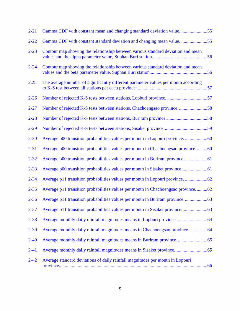
2-21 Gamma CDF with constant mean and changing standard deviation value. ......................55

2-22 Gamma CDF with constant standard deviation and changing mean value. ......................55

2-23 Contour map showing the relationship between various standard deviation and mean values and the alpha parameter value, Suphan Buri station. ..............................................56

2-24 Contour map showing the relationship between various standard deviation and mean values and the beta parameter value, Suphan Buri station. ................................................56

2.25 The average number of significantly different parameter values per month according to K-S test between all stations per each province. ...........................................................57

2-26 Number of rejected K-S tests between stations, Lopburi province. ..................................57

2-27 Number of rejected K-S tests between stations, Chachoengsao province. ........................58

2-28 Number of rejected K-S tests between stations, Buriram province. ..................................58

2-29 Number of rejected K-S tests between stations, Sisaket province. ....................................59

2-30 Average p00 transition probabilities values per month in Lopburi province. ...................60

2-31 Average p00 transition probabilities values per month in Chachoengsao province. .........60

2-32 Average p00 transition probabilities values per month in Buriram province. ...................61

2-33 Average p00 transition probabilities values per month in Sisaket province. .....................61

2-34 Average p11 transition probabilities values per month in Lopburi province. ...................62

2-35 Average p11 transition probabilities values per month in Chachoengsao province. .........62

2-36 Average p11 transition probabilities values per month in Buriram province. ...................63

2-37 Average p11 transition probabilities values per month in Sisaket province. .....................63

2-38 Average monthly daily rainfall magnitudes means in Lopburi province. .........................64

2-39 Average monthly daily rainfall magnitudes means in Chachoengsao province. ...............64

2-40 Average monthly daily rainfall magnitudes means in Buriram province. .........................65

2-41 Average monthly daily rainfall magnitudes means in Sisaket province. ...........................65

2-42 Average standard deviations of daily rainfall magnitudes per month in Lopburi province..............................................................................................................................66

9

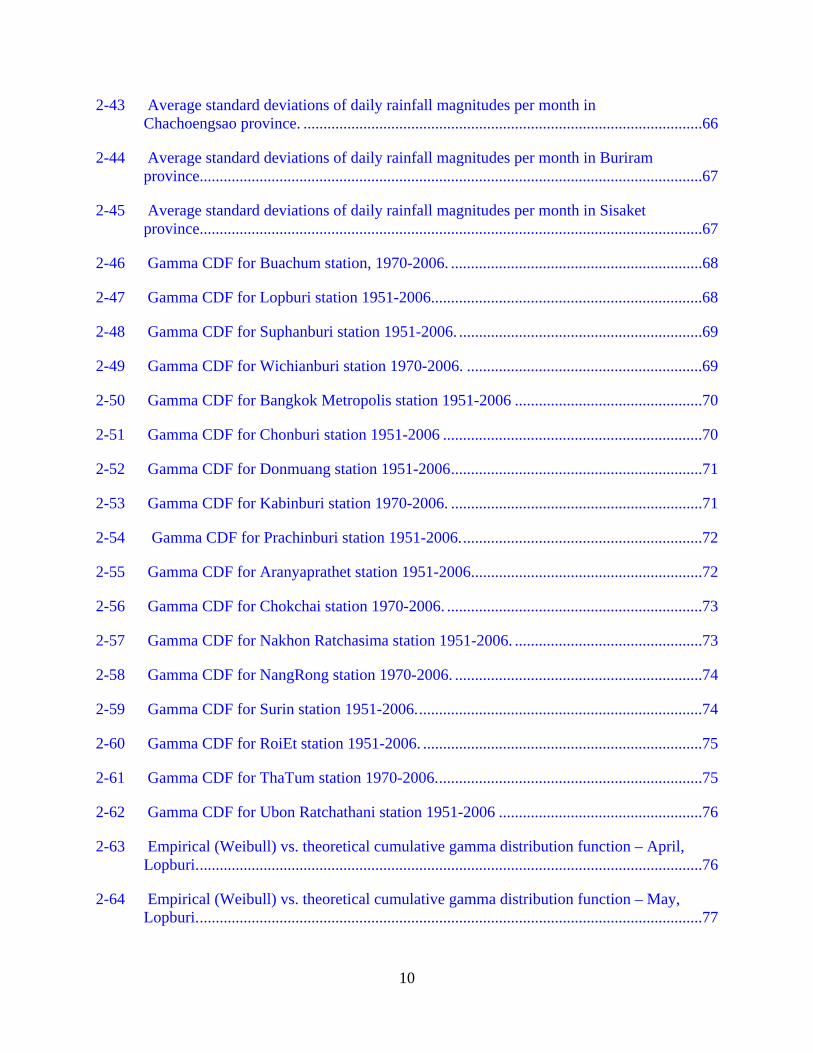
2-43 Average standard deviations of daily rainfall magnitudes per month in Chachoengsao province. ....................................................................................................66

2-44 Average standard deviations of daily rainfall magnitudes per month in Buriram province..............................................................................................................................67

2-45 Average standard deviations of daily rainfall magnitudes per month in Sisaket province..............................................................................................................................67

2-46 Gamma CDF for Buachum station, 1970-2006. ...............................................................68

2-47 Gamma CDF for Lopburi station 1951-2006....................................................................68

2-48 Gamma CDF for Suphanburi station 1951-2006. .............................................................69

2-49 Gamma CDF for Wichianburi station 1970-2006. ...........................................................69

2-50 Gamma CDF for Bangkok Metropolis station 1951-2006 ...............................................70

2-51 Gamma CDF for Chonburi station 1951-2006 .................................................................70

2-52 Gamma CDF for Donmuang station 1951-2006 ...............................................................71

2-53 Gamma CDF for Kabinburi station 1970-2006. ...............................................................71

2-54 Gamma CDF for Prachinburi station 1951-2006. ............................................................72

2-55 Gamma CDF for Aranyaprathet station 1951-2006. .........................................................72

2-56 Gamma CDF for Chokchai station 1970-2006. ................................................................73

2-57 Gamma CDF for Nakhon Ratchasima station 1951-2006. ...............................................73

2-58 Gamma CDF for NangRong station 1970-2006. ..............................................................74

2-59 Gamma CDF for Surin station 1951-2006. .......................................................................74

2-60 Gamma CDF for RoiEt station 1951-2006. ......................................................................75

2-61 Gamma CDF for ThaTum station 1970-2006. ..................................................................75

2-62 Gamma CDF for Ubon Ratchathani station 1951-2006 ...................................................76

2-63 Empirical (Weibull) vs. theoretical cumulative gamma distribution function – April, Lopburi. ..............................................................................................................................76

2-64 Empirical (Weibull) vs. theoretical cumulative gamma distribution function – May, Lopburi. ..............................................................................................................................77

10

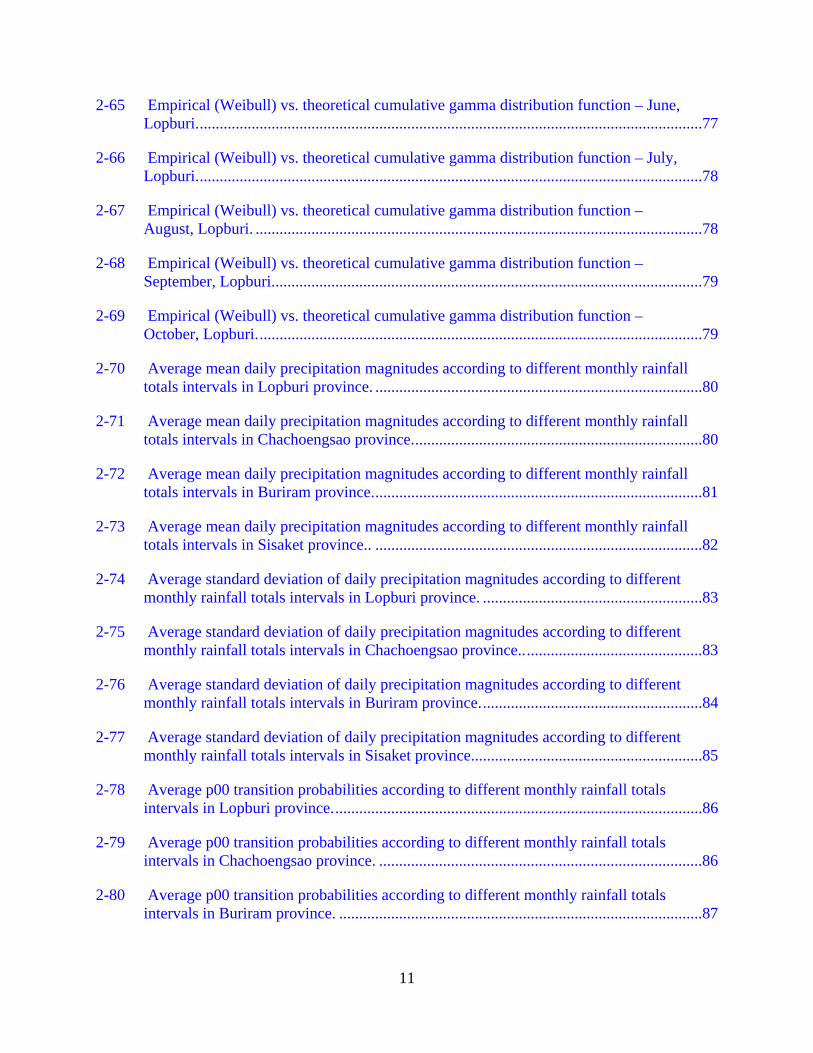
2-65 Empirical (Weibull) vs. theoretical cumulative gamma distribution function – June, Lopburi. ..............................................................................................................................77

2-66 Empirical (Weibull) vs. theoretical cumulative gamma distribution function – July, Lopburi. ..............................................................................................................................78

2-67 Empirical (Weibull) vs. theoretical cumulative gamma distribution function – August, Lopburi. ................................................................................................................78

2-68 Empirical (Weibull) vs. theoretical cumulative gamma distribution function – September, Lopburi. ...........................................................................................................79

2-69 Empirical (Weibull) vs. theoretical cumulative gamma distribution function – October, Lopburi. ...............................................................................................................79

2-70 Average mean daily precipitation magnitudes according to different monthly rainfall totals intervals in Lopburi province. ..................................................................................80

2-71 Average mean daily precipitation magnitudes according to different monthly rainfall totals intervals in Chachoengsao province. ........................................................................80

2-72 Average mean daily precipitation magnitudes according to different monthly rainfall totals intervals in Buriram province. ..................................................................................81

2-73 Average mean daily precipitation magnitudes according to different monthly rainfall totals intervals in Sisaket province.. ..................................................................................82

2-74 Average standard deviation of daily precipitation magnitudes according to different monthly rainfall totals intervals in Lopburi province. .......................................................83

2-75 Average standard deviation of daily precipitation magnitudes according to different monthly rainfall totals intervals in Chachoengsao province.. ............................................83

2-76 Average standard deviation of daily precipitation magnitudes according to different monthly rainfall totals intervals in Buriram province. .......................................................84

2-77 Average standard deviation of daily precipitation magnitudes according to different monthly rainfall totals intervals in Sisaket province..........................................................85

2-78 Average p00 transition probabilities according to different monthly rainfall totals intervals in Lopburi province. ............................................................................................86

2-79 Average p00 transition probabilities according to different monthly rainfall totals intervals in Chachoengsao province. .................................................................................86

2-80 Average p00 transition probabilities according to different monthly rainfall totals intervals in Buriram province. ...........................................................................................87

11

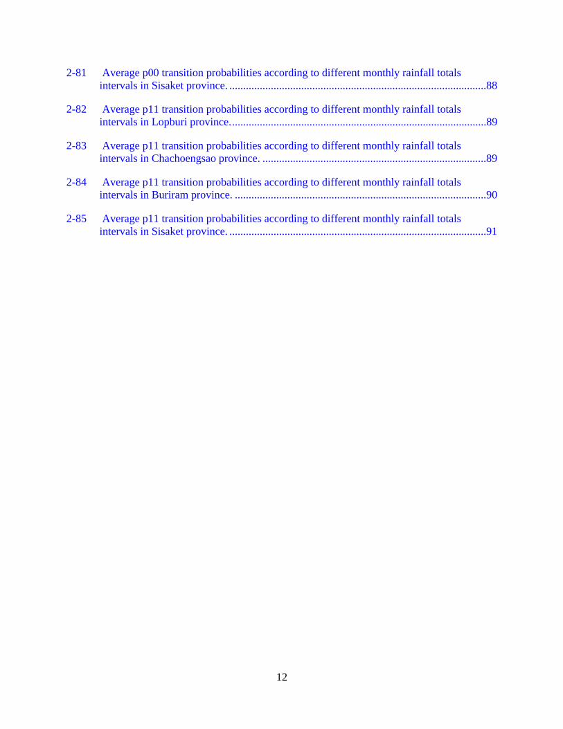
2-81 Average p00 transition probabilities according to different monthly rainfall totals intervals in Sisaket province. .............................................................................................88

2-82 Average p11 transition probabilities according to different monthly rainfall totals intervals in Lopburi province. ............................................................................................89

2-83 Average p11 transition probabilities according to different monthly rainfall totals intervals in Chachoengsao province. .................................................................................89

2-84 Average p11 transition probabilities according to different monthly rainfall totals intervals in Buriram province. ...........................................................................................90

2-85 Average p11 transition probabilities according to different monthly rainfall totals intervals in Sisaket province. .............................................................................................91

12

Abstract of Thesis Presented to the Graduate School of the University of Florida in Partial Fulfillment of the

Requirements for the Degree of Master of Science

DETERMINING THE DAILY RAINFALL CHARACTERISTICS FROM THE MONTHLY RAINFALL TOTALS IN CENTRAL AND NORTHEASTERN THAILAND

By

Anna Maria Szyniszewska

December 2009 Chair: Peter R. Waylen Major: Geography

Daily rainfall attributes are crucial in the risk assessment of climate conditions that may

have damaging effect on agriculture. Although daily rainfall totals data accessibility is frequently

limited, monthly rainfall data are most abundant in space and time in Thailand. The daily rainfall

totals in four provinces of central and north-east Thailand (Lopburi, Chachengsao, Buriram and

Sisaket) were analyzed in order to establish their relationship to rainfall monthly totals. The

study area is characterized by a high diversity of crops, thus there is no single criterion that can

be set for what may constitute an agro-meteorological shock. Daily rainfall is often modeled as a

Markov process involving transitions from wet and dry days and the representation of daily

rainfall totals, all of which are expected to vary seasonally and spatially. The transition

probabilities for consecutive days with rain or no rain were calculated for each month. The

magnitudes of daily rainfalls are represented by the gamma distribution, which parameters can be

simply estimated from the mean and variance. The relationship between the observed monthly

rainfall and the transition probabilities, mean and standard deviation of daily rainfall is examined

using deterministic approach finding the most likely values of parameters of interest according to

6 different intervals of monthly rainfall totals. These probability expressions provide useful

13

14

information on climatic shock occurrence likelihood on the basis of widely available, monthly

rainfall data in Thailand.

CHAPTER 1 INTRODUCTION

Problem Statement

The distribution of rains and climatic shocks play a critical role in the Thai economy,

therefore the ability to assess probability of climatic shock is very important for agriculture and

the food supply. The country has a climate determined by its position in tropical latitudes

between two ocean masses and its exposure to the monsoon winds. High temperatures and heavy

rains with a high level of regional variability are common to this region (Lau and Yang 1997;

Khedari 2000). The investigation of the abundance and magnitude of rain on a daily basis can

give a signal whether a climatic shock has occurred or not. The nature of the relationship

between monthly rainfall totals and daily rainfall characteristics in this region is investigated in

this study.

Importance

The distribution of rains is an important factor in countries water resources and plays an

important role in agricultural planning and management. Thailand has the largest proportion of

agricultural land of all countries in Southeast Asia: from 20 to 25 million hectares, or 40 to 50%

of the country’s total area (Kermel-Torres 2004). Given that 42.6% of the Thai labor force is

employed in the agriculture sector, climatic variability has a direct and indirect impact on

household incomes. The significance of this sector is also on the international level, as Thailand

is a leading exporter of food in Asia and has a rich variety of crops cultivated on its area due to

the policy of crops diversification (Kono and Saha 1995). Despite the country’s effort to develop

sustainable irrigation starting in the 1950s, Thai agriculture still remains highly vulnerable to

seasonal fluctuations in precipitation with 23% of cultivable land classified as irrigated in 1996

(Kermel-Torres 2004). Many rice cultivation areas require additional irrigation even during the

15

16

monsoon season. As the country’s economy is highly dependent on revenue from the agricultural

sector, it is vital to understand the nature of the short-time climate variability in this region.

Research Objectives

The goal of this study was to find the probability of climate shock occurrences in four Thai

provinces: Chachoengsao, Buriram, Sisaket and Lopburi. These particular provinces were chosen

because each contained one county that had been sampled every year by the comprehensive Thai

Socio-Economic Survey, thus providing comparative information of climatic variables. A major

task of the large interdisciplinary project that this study is part of is to quantify the risk of climate

variation and change and then link that to actual versus potential insurance, economic, and social

decisions. The variability of the precipitation causing damage to the agriculture and was

estimated in this research. The events of interest are extremes of high or low rainfall that exceed

thresholds that have agricultural or other significance, e.g., a series of rainfall events that causes

floods, or a series of dry days that cause droughts. For the events when rain occurred, the

probability of extremely low and extremely high rainfall magnitudes was estimated for certain

thresholds of monthly rainfall totals.

CHAPTER 2 DETERMINING THE DAILY RAINFALL CHARACTERISTICS FROM THE MONTHLY

RAINFALL TOTALS IN CENTRAL AND NORTHEASTERN THAILAND

Introduction

The distribution of rains and climatic shocks resulting from deviations to the anticipated

spatial and temporal patterns play important roles in the Thai economy (Paxson 1992).

According to the CIA World Factbook estimates from 2005, over 42% of the country’s labor

force is employed in the agricultural sector which directly relies on summer monsoon to bring

moisture to support the crop growth. When the climate deviates from its normal pattern,

agricultural activities are disrupted and household incomes are directly affected (Gadgil and

Kumar 2006).

Thailand, with its tropical position is subjected to large interannual and seasonal variability

in precipitation and thus often experiences excess or dearth of rain that cause severe floods or

droughts respectively which affect agriculture (Boochabun et al. 2004). Moreover, the country is

characterized by a high diversity of crops and irrigation methods, thus no single criterion can be

set for what constitutes an agro-meteorological “shock”. This study, which is part of a larger

interdisciplinary project, investigates the empirical relationship between monthly rainfall totals

which are more abundant in both space and time, and chosen daily rainfall characteristics that

describe the probabilities of conditions that might be considered agricultural shocks. A major

task is to quantify the risk of climate variation and then link that to actual versus potential

insurance, economic and social decisions.

Two main properties of the daily totals are investigated on a monthly basis: 1) Is it raining

on given day? 2) If yes, how much rain falls? Daily rainfall occurrences are modeled as a

Markov process involving transitions between wet and dry days, and daily rainfall totals by an

appropriate probability distribution. These properties are calculated at 17 synoptic stations over

17

periods of 1951-2006 or 1970-2006 depending on location. Four provinces are selected for this

study, two in the central Thailand and two in the northeast Thailand. For each province, daily

rainfall data from the four closest synoptic stations were examined.

Ideally, the properties of wet-day rainfall totals can be represented by a probability

distribution, sufficiently flexible to be used in all locations through the rainy season. The

parameters should be estimated easily and be physically interpretable, in order that they may be

linked deterministically to observed monthly totals. High probabilities of long sequences of rainy

days, combined with high probabilities of large magnitudes of daily rain create a setting in which

excess of rains and floods are likely. Conversely, high probabilities of sequences of dry days

accompanied by low magnitudes of precipitation create a setting favorable for drought. Derived

empirical estimates provide useful information on the most likely combination of daily rainfall

characteristics for a particular magnitude of monthly rainfall, which are more ubiquitous in

Thailand.

Literature Review

Rainfall Variability in Southeast Asia

Thailand is situated between the two large ocean water bodies of the Pacific and Indian

Oceans. Its climate is dominated by two air streams: a dry northeast monsoon that commences in

November and lasts until February, and the wet southwestern Asian monsoon that commences in

mid-May and lasts until mid-October (Lu et al. 2006). The monsoons are controlled by the

Intertropical Convergence Zone (ITCZ), which migrates over Thailand northwards in May and

southwards during September (Lau and Yang 1997; Kermel-Torres 2004; Khedari 2000). The

country is subjected to strong intra- and interannual variability in precipitation, potentially

conditioned upon the El Niño-Southern Oscillation (ENSO) phenomenon. The relationship

between ENSO, one of the most important modes of global climate variability, and the Indian

18

summer monsoon has been widely studied for India, but there are far fewer studies investigating

links to summer rainfall in Thailand (Kripalani and Kulkarni 1997). While the relationship

between the Indian monsoon and ENSO has weakened in past decades (Kumar 1999), the

negative association between warm phases of ENSO and summer rainfall over Thailand may

have strengthened since 1980 (Singharattna et al. 2005).

Rainfall and the Agriculture

Agriculture is one of the most climate dependent human endeavors (Mendelsohn 2007;

Murdiyarso 2000). More than half of world’s population relies on the Asian monsoon to sustain

agriculture, the dominant source of income in Southeast Asia. Rice is the main food staple in this

region - it accounts for about 90% of the agricultural area and 92% of global rice production,

with Thailand being the world’s largest rice exporter.

Rain is the most limiting factor for rice production in South and Southeast Asia therefore

when the summer monsoon deviates from its normal pattern, the agricultural operations are

disrupted accordingly. Too much or too little rain causes the crop to suffer moisture stress that

can have disastrous effects on the people and economy. In general, the impacts of drought are

known to be more harmful than those of excess rainfall (Gadgil and Kumar 2006). While rice

predominates in the study area, Thailand has recently undergone a process of crop diversification

particularly in the center of the country – mainly the Chao Praya river basin, which is the heart of

national agricultural and economic activities. Other major crops include sugar cane, cassava,

rubber, maize, mung bean and soybean. Thus, there is no single criterion that would be

responsible for agricultural “shock” in this area as various crops are resistant to different levels

of moisture stress. However, Gadgil and Kumar (2006) indicated that there are three most

important characteristics of rain that can have affect on the agriculture: rainfall magnitude, spells

of dry and wet days, and the monsoon onset.

19

Spells of Dry and Wet Days

A Markov chain is a stochastic process widely used in climatology to represent the time

series of discrete states, in this case the sequence day, or states, with “rain” or “no rain”. It

provides information about the risks of dry or wet spells, both of which are potential agricultural

shocks. An important characteristic of this model is the degree of dependence of each

observation upon the state observed previously, controlled by the order of the model (Haan 1977,

Wilks 1998, 1999, 2006). Most commonly a simple 1st order is generally assumed, although

higher orders have also been used (Katz 1981). A two-state first-order Markov model consists of

four parameters: p00 (the probability of a dry day following a dry day), p01 (the probability of a

wet day following a dry day), p10 (the probability of a dry day following a wet day) and p11 (the

probability of a wet day following a wet day). As the values p00 with p01, and p11 with p10,

always sum to 1 only one of each pair is required to fully characterize the process. Numerous

studies have shown the applicability of the first order Markov chain to rainfall modeling (Caskey

1963; Katz 1977, 1981; Coe and Stern 1981; Harrison and Waylen 2000).

Daily Precipitation Magnitudes

The magnitude of daily, non-zero precipitation totals can be represented by one of many

exponential-types of continuous probability distributions such as the gamma, Generalized Pareto,

Pearson or generalized extreme value (Katz 1977; Coe and Stern 1982; Stern and Coe 1984;

Rosbjerg et al. 1992; Madsen et al. 1997; Stephenson et al. 1999), which have a lower bound of

zero as there is no negative precipitation. Distributions such as the Generalized Pareto and

gamma are sensitive to the important values in the tail of the distribution. Both are described by

two parameters that are derived from the sample mean and variance via the method of moments

(Barger and Thom 1949, Thom 1958, Ison et al. 1971, Shenton and Bowman 1973, Rosbjerg et

al. 1992; Madsen et al. 1997; Stephenson et al. 1999). Among many distributions that were

20

attempted to be fit to the empirical data the gamma distribution was found to have the best fit

across the study area and was thus chosen to represent daily rainfall total magnitudes.

Study Area and Data

Four Thai provinces (changwats): Chachoengsao and Lopburi located in central Thailand

and Buriram and Sisaket in the Northeast are chosen as each contains one county (amphoe) that

had been sampled every year by the comprehensive Thai Socio-Economic Survey, providing a

benchmark for comparative studies between environmental and socio-economic variables. The

Central and northeast areas range from relatively wealthy to relatively poor, not only in terms of

income measures, but also in moisture availability, soil fertility, land cover, and other

environmental characteristics. The center of the country stretches over a vast alluvial plain

drained by the Chao Phraya River, while the northeast of Thailand occupies the Khorat plateau.

The central area has a relatively high diversity of crops and is fairly well irrigated, whereas the

northeast is less diversified and the percent of irrigated arable land is relatively low (Gleick

1993). In the former, the percent of households deriving income from agriculture is estimated to

be between 38 and 53% and in the latter between 65 and 81% (Kernel-Torres 2004).

Daily precipitation data are obtained from the Thailand Meteorological Department for

seventeen synoptic stations in central and northeast Thailand region for the period of 1951-2006

or 1970-2006 depending on the location (Fig. 2-1 and 2-2). The stations used in the study are

selected according to the distance from the socio-economic survey villages and the duration of

full daily rainfall record. Stations with at least 30 years of daily rainfall record and within a

distance no larger than 100 km are sought in order to provide a reasonable estimation of daily

rainfall characteristics in the survey villages.

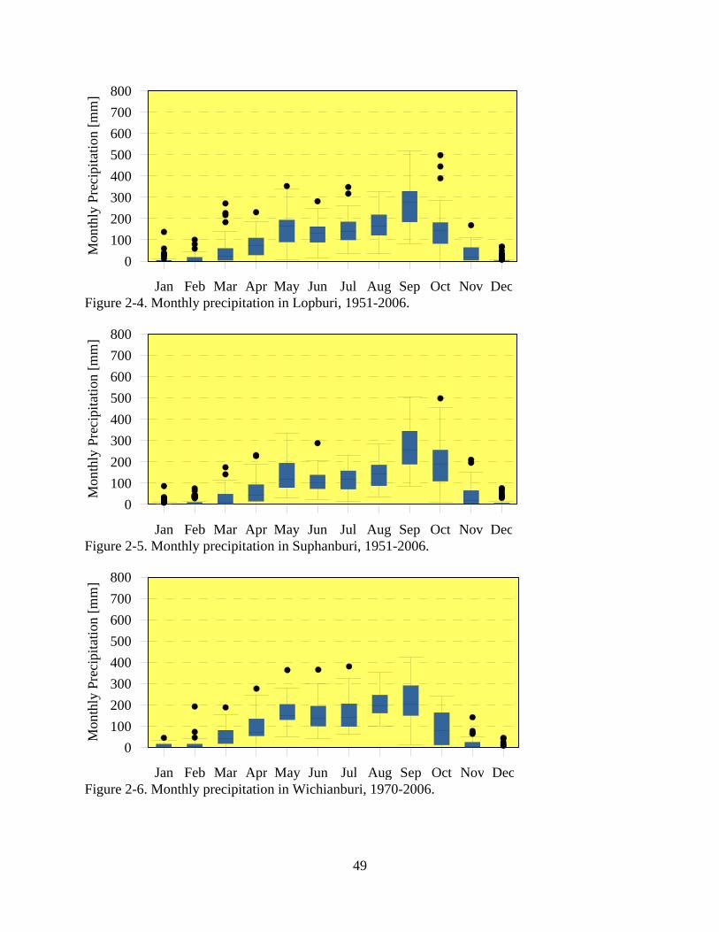
The monthly precipitation regimes of the stations are represented in Figures 2-3 through 2-

18. Those of the center of the country exhibit a visible reduction in precipitation in the middle of

21

the rainy season, which corresponds to the ITCZ’s most northerly position before moving

southward in the end of the season. The regime of the northeast evinces a less pronounced

bimodal distribution of rainfall. Precipitation generally peaks during September and the central

provinces show a secondary maximum in May. The research focuses on the seven wettest

months starting with April until the October, that include the summer monsoon season, which

accounts for over 80% of annual precipitation.

Methodology

A wet day in this study is defined to be one on which there is at least 0.1mm of

precipitation on record. This threshold could possibly be modified according to the application

needs. The transition probabilities for consecutive days with rain or no rain are calculated for

each month. Markov chain models are created by conditioning the probability of the occurrence

of rainfall on one day upon whether measurable rainfall was observed on the previous days.

These are characterized by “transition probabilities” (Equation 2-1).

{ } { }mttttttttt XXXXXXXXXX −−−+−−+ = ,...,,Pr,...,,Pr 2111211 (2-1)

The most common Markov chain used in research is first order two-state model (Gates and

Tong 1976; Katz 1977; Guzman and Torrez 1985; Hosking and Wallis 1987; Harrison and

Waylen 2000). This yields four parameters, two of which are employed in this study: the

probabilities of no rain being followed by no rain (p00), and that of rain followed by rain (p11).

Higher probabilities of p00 indicate higher likelihood of long dry spells and drought in terms of

monthly totals. On the other hand, higher probabilities of p11 indicate a greater likelihood of

long sequences of wet days and therefore supersaturated soils that may lead to floods.

Rainfall totals are modeled by the exponential-like gamma distribution (Haan 1977;

Rosbjerg et al. 1992; Madsen et al. 1997; Wilks 2006). (Figure 2-19 and 2-20). Equation 2-2

22

defines the gamma cumulative distribution function (CDF) and 2-3 the density function. The two

parameters alpha (α) and beta (β) can be easily estimated from sample mean and variance using

method of moments (Equation 2-3 and 2-4).

0,,/ˆ/ˆ

)()/exp()/()(

)()/exp()()(

2

22

1

1

>=

=

Γ−

=

Γ−−

=

−

−

βαβ

ααβ

ββαβ

ββ

α

α

xxs

sx

xxxf

xxxf

(2-2)

(2-3)

(2-4)

(2-5)

Parameters are estimated from precipitation magnitudes observed during a specific month,

across all years of record.

Alpha controls the shape of the distribution. For α < 1 the distribution is strongly skewed

to the right as illustrated on Figure 2-20. The values of alpha increase as the sample mean

increases but decrease as the standard deviation increases. The larger alpha the more skewed is

the distribution and, as a result, the lower probability of receiving small rainfall values. The

special case of α = 1 arises for an exponential distribution and it has been illustrated on the same

figure. In that case the distribution is flatter and less sensitive to the daily rainfall properties in

the tail.

Beta, the scale parameter, controls the spread of the distribution (Figure 2-20), stretching

or squeezing the distribution to the right or left depending on the magnitudes of the observed

data. The value of this parameter exponentially increases as the sample standard deviation value

increases and decreases as the sample mean increases.

Figures 2-21 and 2-22 illustrate how the shape of the distribution changes with a changing

sample standard deviation function (with constant mean) and with a changing mean (with

23

constant standard deviation). The mean has stronger influence on the shape of the distribution

while standard deviation regulates its extent.

The empirical distribution of the rainfall magnitudes to which fitted distributions are

compared, is calculated using the Weibull plotting position where Pemp is the exceedance

probability of the ith ranked observation (lowest rainfall magnitude to the highest) with the

highest rank, N, being the number of total observations in the sample (Cunnane 1978).

Pemp = i/(N+1) (2-6)

The estimated gamma distributions, with parameters varying according to month and

locations, are then compared with the empirical cumulative distribution of rainfall magnitudes

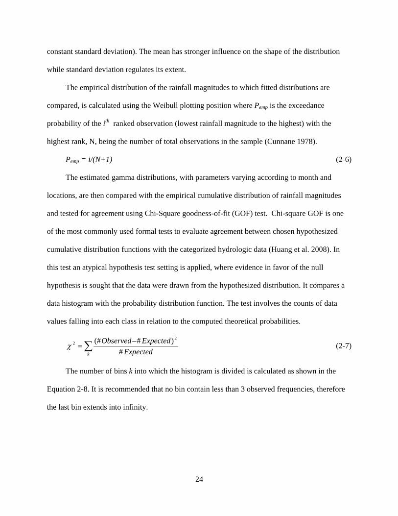
and tested for agreement using Chi-Square goodness-of-fit (GOF) test. Chi-square GOF is one

of the most commonly used formal tests to evaluate agreement between chosen hypothesized

cumulative distribution functions with the categorized hydrologic data (Huang et al. 2008). In

this test an atypical hypothesis test setting is applied, where evidence in favor of the null

hypothesis is sought that the data were drawn from the hypothesized distribution. It compares a

data histogram with the probability distribution function. The test involves the counts of data

values falling into each class in relation to the computed theoretical probabilities.

∑ −=

k ExpectedExpectedObserved

#)#(# 2

2χ (2-7)

The number of bins k into which the histogram is divided is calculated as shown in the

Equation 2-8. It is recommended that no bin contain less than 3 observed frequencies, therefore

the last bin extends into infinity.

24

σ×= 4.0k (2-8)

The number of degrees of freedom (DOF) is calculated using the number of bins minus the

number of the parameters of fit minus 1 (Equation 2-9).

DOF = (# of bins - # of parameters of fit – 1) (2-9)

Four properties of daily rainfall, which summarize the risks of agricultural shock, are

therefore examined: the first order transition probability from state of no rain to no rain (p00),

the first order transition probability from state of rain to rain (p11), as well as mean and standard

deviation of the daily rainfall magnitudes on days when rain occurred. Parameters of interest are

calculated at every station for individual months. The primary research problem is to associate

the most likely combinations of these statistics (and thus parameters) with the respective monthly

rainfall totals, in order to provide a means of “downscaling” from the monthly rainfall totals,

which are more abundant both in space and time across Thailand, to the likely, and unknown,

daily rainfall characteristics in the past .

Monthly rainfall totals are then grouped into six different arbitrarily chosen intervals (0-

100mm, 100-200mm, 200-300mm, 300-400mm, 400-500mm and 500-900mm) and relative

frequency distributions of the values each of the four parameters of interest corresponding to

these intervals, by month, are constructed, the mean parametric value in each interval is

calculated and plotted in a summarizing graph that illustrates empirically the most likely

parameter value for a given interval of monthly total for each month.

In order to test for any heterogeneity of these characteristics within a province, a two-

sample Kolmogorov-Smirnov (K-S) test is employed. The test compares the observed

distributions of the four calculated monthly parameters – mean, standard deviation, p00 and p11

- between the stations in each province searching for evidence that these parameters vary

25

significantly between stations, in a given month. The K-S test uses the test statistic D indicating

the largest absolute distance between the two empirical functions (Equation 2-9):

Dn = max |Fn(x)-F(x)|, (2-9)

where Fn(x) is one empirical cumulative probability and F(x) is the other. The null

hypothesis is that the observed data were drawn from the same distribution (Wackerly 2002).

Results

Intra-Provincial Variability

The K-S goodness-of-fit test indicates very few significant differences in the distributions

of similar parameters within any province (tables 2-1 to 2-4). Figure 2-25 depicts the average

number of occasions that the rejected null hypothesis is rejected in each province. The

maximum possible value would be 42 (6 ways of cross-comparing four stations times 7 months

of comparison), or 70 in the Buriram and Chachoengsao provinces for which there are 5

recording stations. Figures 2-26 through 2-29 are constellation diagrams illustrating the number

of significantly different monthly parameter values between each pair of stations, their inter-

station distances and geographic disposition. By far the largest intra-provincial heterogeneity is

observed in Chachoengsao (figure 2-27) with a marked difference between the group of stations

located close to the Gulf of Thailand (Bangkok, Donmuang and Chonburi) compared to group of

two stations located in the north of the province – Prachinburi and Kabinburi. While there is

greater overall homogeneity the Lopburi province (Figure 2-26), inter-station distance appears to

exert the greatest control. In Buriram (Figure 2-28), the highest differences are again generally

observed between the most distant stations like Surin, Nakhonratchasima and Aranyaprathet,

while Sisaket preserves the strongest intra-provincial homogeneity among all four provinces

(Figure 2-29). It seems reasonable therefore to treat the parameters derived from statistically

alike stations in each province, as if they were all records or realizations drawn from the same

26

“provincial population”, and combine them to obtain a greater sample size. Further evidence for

this assumption is pursued through an investigation of the seasonal changes in the mean values

of the rainfall model parameters.

Seasonal Changes in Transition Probabilities

Various spatial and temporal trends are apparent in magnitudes of p00 and p11 parameters.

Figures 2.30 through 2.37 represent averaged transition probabilities for each month, within a

province.

April as the month of the onset of the monsoon has been shown to possess high inter-

annual variability and is by far the driest month chosen for this study. It is therefore expected,

that in April we observe the highest values of p00 in the season. In Chachoengsao and Lopburi

province p00 value is above .80, whereas in the Sisaket and Buriram this value is about .70. This

tendency is different from the anticipated spatial variability as it would be expected that

geographically the monsoon season commences first in the central provinces.

As the monsoon season progresses, the values of p00 decrease at slightly different rates

depending on location, although there appears to be no major difference between provinces or

central and northeastern regions. Values in Lopburi show a leveling between May and June and

gently decrease afterwards, while Sisaket displays the most constant values of p00 at about .50

starting in May through September. Buriram experiences the greatest fluctuations both

temporally and spatially although the same overall trend is apparent. Values in Chachoengsao are

gently decreasing from .70-.85 in April up to .35-.45 in September indicating lower probability

of dry-dry transitions every month. This decreasing trend comes to an abrupt end in October at

all stations and provinces as the monsoon retreats, thus increasing the probability of two

consecutive dry days.

27

As might be expected, the values of p11 tend to mirror those of p00. Values in April in all

of the provinces are approximately .30-.40 with Lopburi province having the highest internal

variability in the range of .25-.35 in the southwest and .35-.45 in the northeast. As the monsoon

season commences fully in May values are the highest in Chachoengsao province (.60-.70) and

slightly less (.50-.60) in the other provinces, increasing gradually until September in Sisaket,

Buriram and the easternmost stations of Chachoengsao, while the rise is delayed until in June in

the more westerly Lopburi and western portions of Chachoengsao. September represents the

highest p11 parameter values at all locations at the range of .60-.80 and are very homogeneous at

the intra-provincial level.

The end of the monsoon season is marked by a decline, although not as sharp as the

increase observed in p00. The p11 values are in the range of May and June values and decrease

to the range of .45-.70 with the highest values and the lowest intra-provincial variability in

westernmost Chachoengsao and the largest intra-provincial variability together with lowest

values in easternmost Sisaket.

Gamma Distribution

The Chi-squared results as detailed in (tables 2-9 through 2-12) and example plots the

distributions of daily total are presented in Figures 2-63 through 2-69 for the seven months at

Lopburi station. In only 10% of the cases (13 of 126) was the null hypothesis of no significant

differences rejected. Eight of these cases were months in Buriram province, in which the fitted

gamma failed to approximate the observed records at Nangrong. No month appeared particularly

more susceptible than other, although 6 of the poor fits did occur in April and May.

Rainfall Magnitudes Parameter Values

Figures 2-23 and 2-24 graph the relationship between increasing standard deviation (s) and

mean (x) daily rainfall values and the values of alpha (α) and beta (β) respectively. Most records

28

produced combinations of mean and standard deviation that plot between alpha values of 0.4 and

0.6 – roughly on the 45 degrees slope. The alpha values for at Suphanburi indicate higher

variances in proportion to means early in the monsoon season (α <0.5) and lower variances at the

end of the season (α >0.5). Figure 2-24 displays the same relationship for the beta parameter. The

higher density of contour lines on y axis indicates the greater sensitivity of β to the value of the

standard deviation. June, July and August have the lowest values of standard deviation and also

the lowest β parameter, therefore the distribution will be least dispersed. May and September

have the same β value, although in May we observe lower x and lower s. April has the highest

scale parameter values β and therefore the distribution is more stretched compared to May,

which indicates more likely high rainfall values (Figure 2-48).

The average expected mean and standard deviation values for each station averaged for all

years and represented by month are shown in Figures 2-38 through 2-45. Worth mentioning is

the fact that the standard deviation is always larger than the mean – and as a consequence α

values fall always below 1.0 and more specifically in the range of .40 - .60. At the same time,

values of x and s are highly correlated. Most of the trends indicate the bimodal peaks of both

mean and standard deviation values in May and September. The highest mean rainfall

magnitudes accompanied with the highest s values are expected at the end of the monsoon

season peaking in September. Conversely, the lowest x and s values are in the middle of the

monsoon season starting in June until August.

Stations located in the vicinity of Chachoengsao province have the highest peak mean

daily rainfall between 14-17 mm for that month and a standard deviation of 18.3-22.2 mm. The

lowest mean daily totals are observed in the middle of the monsoon season – from June through

August, with the exception of Kabinburi and Prachinburi stations in Chachoengsao, where the

29

monthly means increase steadily and gradually from April to September, and decrease slightly in

August. Variability between different expected mean daily rainfall magnitudes in the middle of

the monsoon season in this province represents the most prominent source of intra-provincial

variability. The same is the case for the standard deviation scores in these two stations. Similar

trend of changes in x and s is observed in the Lopburi province with higher x and s values at the

end and the beginning of the monsoon season, and considerably lower in the middle (Figures 2-

38 and 2-42).

Parameter Changes According to Monthly Totals

The final results of this study identify the most likely four rainfall parameter values

associated with the observed monthly rainfall totals.

Figures 2-70 through 2-73 show considerable homogeneity in the relationship between the

monthly rainfall totals and the daily mean rainfall magnitudes (x) across all four provinces. With

each 100mm increment of monthly rainfall totals, the expected daily rainfall value is increasing

by about 5 mm. Among the various months, April has the highest slope of increase, indicating

less frequent but more intensive daily precipitation. This characteristic is common to each of the

four provinces.

The standard deviations (Figures 2-74 – 2-77) follow a similar trend, although as might be

expected given that they are second order moments they tend to be a little noisier. Only in April

and October, when daily rainfall occurs least frequently, does the variability increase markedly

compared to other months as the monthly totals increase.

As it could be expected, p00 tends to decline with increasing monthly rainfall totals, and

p11 increases (Figures 2-78 – 2-85). However considerable spatial and temporal variability about

this pattern can be identified, particularly during July, August and September. In Lopburi in

August, p00 tends to increase with monthly rainfall totals, and although p11 values do rise they

30

tend to do so at a lower rate than in other months. Similar behavior is observed in Buriram

during September. The southern province of Chachoengsao a large spatial variability in trends of

changes in p00 values for these three months according to various monthly rainfall totals values.

This could result from the lower sample size in certain monthly rainfall totals intervals.

Discussion

The rainfall magnitudes are well described using the gamma distributions. In the majority

of months the mean and standard deviation of daily rainfall magnitudes increase steadily with

increasing monthly rainfall totals, although there is some individual variability. April is by far

the most unusual month, generally showing a far higher rate of change (but low totals). The

absolute levels of mean daily rainfall magnitudes increase with higher monthly rainfall totals

throughout the summer monsoon season. However, various months are characterized by slightly

different absolute (as opposed to slope) levels of the mean, especially on the interprovincial

level, indicative of the generally wetter conditions in the westerly provinces of Chachoengsao

and Lopburi. Seasonal patterns are dominated by the advance and retreat of the monsoon as well

as migration of ITCZ zone. For instance, at Lopburi station, April has average value of 10 mm

of daily precipitation when the monthly total is between 0 and 100 mm, in May it is 8 mm, and in

August it is less than 5 mm. With increasing monthly rainfall total, April, May and October,

display constantly higher mean daily rainfall magnitudes than other, wetter months. Because of

the limited number of days with rain in these months, the longest dry spells of dry days can be

expected, and increased monthly rainfall totals can be expected as a result of higher totals (mean)

falling in the few days of rain. P00 usually stays at similar high levels in these months regardless

of monthly rainfall totals (low slopes to lines). The likelihood of consecutive rainy days is the

lowest in April; however it rises sharply as the monthly total increases. Rain is less frequent than

in other months, but on average – more intense. Greater variability is observed in changes of the

31

transition probabilities on the intra-annual scale, than in means and standard deviations, implying

that the frequency with which the rainfall generating process is changing through the season.

The least intense but most persistent rains occur in September as implied by the stable values of

p00 and p11. In October the rain is less persistent and the average expected rainfall magnitudes

are relatively high. These analyses in combination with the previous analysis of intra-provincial

homogeneity, suggest that a single provincial relationship between monthly rainfall total and

each of the four parameters can reasonably be derived by taking an average of the relationships

for each station.

Figures 2-70 through 2-85 show the most likely parameters of the daily rainfall models

associated with a given interval of monthly rainfall totals at a specific time and location. The risk

of some specific “shock” to occur in the future (e.g. unusual sequence of dry days, or unusually

large daily rainfall totals) can be simply derived as shown in the examples below. For instance,

for a crop that cannot sustain moisture stress that would exceed 10 consecutive days without rain,

the risk of this stress to occur can be estimated multiplying the p00 transition probability at the

closest synoptic station according to the monthly rainfall total interval. For the monthly rainfall

total of 167mm in the southwest part of Lopburi province, in May this risk would be estimated

0.66 to the power of 10 which returns 1.58% chance. For the same monthly rainfall total in the

wetter months of July and September this chance would be even lower: 0.28% and 0.08%

respectively. The chance of the same conditions in the same months but for higher monthly

rainfall totals decreases. For the interval of 300-400mm it is 0.06% in May, 0.04% in July and

0.01% in September. Conversely, the risk of high moisture conditions can be calculated with the

application of p11 and a gamma distribution. If the risk of 2 consecutive days of rain each

exceeding 25 mm is to be calculated for the same three months and location, the p11 need to be

32

risen to the power of 2, and multiplied by the probability of 25mm exceedance derived from the

gamma distribution raised to the power of 2. The gamma distribution needs to be described by

the most likely mean and standard deviation values. The results return an extremely low chance

of this event to happen for the monthly rainfall total interval of 100-200mm: 0.01% in May,

0.00% in July and 0.02% in September. For the monthly rainfall total interval of 300-400mm

these chances increase: 0.17% in May, 0.09% in July and 0.31% in September.

The risk of various sets of conditions can be calculated for the future using the same

approach and selecting the average parameter values at a specific location. This is an easy and

straightforward way to assess the risk of a certain agro-meteorological condition to occur as well

as track the most likely conditions that occurred in the past.

Conclusions

Excess or dearth of rain can have a negative effect on local agriculture, which is the source

of majority household incomes in Thailand. The main research goal of the larger

interdisciplinary project was to link the climatologic variables with the socio-economic surveys

conducted in four provinces of Thailand: two in the center and two in the northeast of the

country. The climatological modeling problem was to assess the risk of occurrence of certain

agro-meteorological conditions, or “shocks” that could create a moisture stress setting for a

variety of crops in the region. The results of this study provide a straightforward and easy for a

non-statistician method of predicting the risk of these conditions to happen and it could be

adopted by various end-users, for instance local farmers or insurance companies that can apply

these findings according to their needs. In addition, given the paucity and lack of reliability of

the daily rainfall records in the villages themselves, this research establishes means by which the

parameters that defined the risks of various shocks can be estimated based solely upon the more

widely available records of monthly rainfall totals.

33

The strength of this method is that four daily rainfall characteristics can be simply

estimated using the transition probabilities, means and standard deviations of daily rainfall totals.

This direct approach makes it attractive to various users including non-statisticians. The derived

probability expressions furnish useful information on risks of variously defined daily rainfall

climatic shocks in the future, with the application of average conditions expected at seven

wettest months in a year during the last decades. Likewise, for the purpose of hindcasting the

daily rainfall conditions in the past, these probabilities can be assessed according to various

monthly rainfall totals and respective most likely four parameter values.

The results from this study have show that the rainfall generating process in time and space

are reasonably homogenous within (and to a lesser degree, between) those four regions, and that

a single provincial relationship between monthly rainfall totals and the four parameters are all

that is needed. Two parameters describing daily rainfall magnitudes: mean and standard

deviation are shown to be highly correlated not only one with another, but also with increasing

monthly rainfall totals. The biggest cause of the intra-annual variability is not so much variability

in the daily rainfall totals, as in the frequency and persistence of rainy days, described by p11

and p00. As expected, p00 and p11 values tend to decrease and increase respectively with

increasing monthly rainfall totals, however relatively large variability in the behavior of these

parameters is observed at various locations. The periods of consecutive days with or without

rain, is highly variable both throughout the season and also according to various magnitudes of

monthly rainfall totals.

34

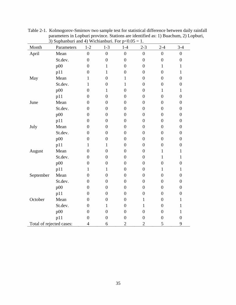
Table 2-1. Kolmogorov-Smirnov two sample test for statistical difference between daily rainfall parameters in Lopburi province. Stations are identified as: 1) Buachum, 2) Lopburi, 3) Suphanburi and 4) Wichianburi. For p<0.05 = 1.

Month Parameters 1-2 1-3 1-4 2-3 2-4 3-4 April Mean 0 0 0 0 0 0 St.dev. 0 0 0 0 0 0 p00 0 1 0 0 1 1 p11 0 1 0 0 0 1 May Mean 1 0 1 0 0 0 St.dev. 1 0 1 0 0 0 p00 0 1 0 0 1 1 p11 0 0 0 0 0 0 June Mean 0 0 0 0 0 0 St.dev. 0 0 0 0 0 0 p00 0 0 0 0 0 0 p11 0 0 0 0 0 0 July Mean 0 0 0 0 0 0 St.dev. 0 0 0 0 0 0 p00 0 0 0 0 0 0 p11 1 1 0 0 0 0 August Mean 0 0 0 0 1 1 St.dev. 0 0 0 0 1 1 p00 0 0 0 0 0 0 p11 1 1 0 0 1 1 September Mean 0 0 0 0 0 0 St.dev. 0 0 0 0 0 0 p00 0 0 0 0 0 0 p11 0 0 0 0 0 0 October Mean 0 0 0 1 0 1 St.dev. 0 1 0 1 0 1 p00 0 0 0 0 0 1 p11 0 0 0 0 0 0 Total of rejected cases: 4 6 2 2 5 9

35

Table 2-2. Kolmogorov-Smirnov two sample test for statistical difference between daily rainfall parameters in Chachoengsao province. Stations are identified as: 1) Bangkok Metropolis, 2) Donmuang, 3) Chonburi, 4) Prachinburi and 5) Kabinburi. For p<0.05 = 1.

Month Parameters 1-2 1-3 1-4 1-5 2-3 2-4 2-5 3-4 3-5 4-5 April Mean 0 0 1 0 0 1 0 0 0 1 St.dev. 0 0 0 0 0 0 0 0 0 0 p00 0 0 1 1 0 1 0 1 1 0 p11 0 0 0 0 0 0 0 0 0 0 May Mean 0 0 0 0 0 0 0 0 0 0 St.dev. 0 0 0 0 0 0 0 0 0 0 p00 0 0 1 1 0 0 0 1 0 0 p11 0 0 0 1 0 0 1 0 0 0 June Mean 0 0 1 1 0 1 1 1 1 0 St.dev. 0 0 1 0 0 1 1 1 0 0 p00 0 1 1 0 0 1 0 0 0 0 p11 0 0 1 1 0 1 1 1 1 1 July Mean 0 0 1 1 0 1 1 1 1 0 St.dev. 0 0 1 1 0 1 1 1 1 0 p00 0 0 1 1 0 1 1 1 0 0 p11 0 0 1 1 0 1 1 1 1 0 August Mean 0 0 1 1 0 1 1 1 1 0 St.dev. 0 0 1 1 0 1 1 1 1 1 p00 0 0 1 0 0 1 1 0 0 0 p11 0 0 1 1 0 1 1 1 1 0 September Mean 0 0 0 0 0 1 0 0 0 0 St.dev. 0 0 0 0 0 0 0 0 1 0 p00 0 0 0 0 0 0 0 0 0 0 p11 0 0 0 0 0 0 0 0 0 0 October Mean 0 0 1 1 0 0 0 0 1 0 St.dev. 1 0 1 1 0 0 0 0 1 0 p00 1 1 0 1 0 0 0 0 0 0 p11 0 0 0 0 0 0 0 0 0 0 Total rejected: 2 2 17 15 0 15 12 12 12 3

36

Table 2-3. Kolmogorov-Smirnov two sample test for statistical difference between daily rainfall parameters in Buriram province. Stations are identified as: 1) Aranyaprathet, 2) Chokchai, 3) Nangrong, 4) Surin and 5) Nakhon Ratchasima. For p<0.05 = 1.

Month Parameters 1-2 1-3 1-4 1-5 2-3 2-4 2-5 3-4 3-5 4-5 April Mean 0 0 0 0 0 0 0 0 0 0 St.dev. 0 0 0 1 0 0 0 0 0 0 p00 0 0 0 0 0 0 0 0 0 0 p11 0 0 0 0 0 0 0 0 0 0 May Mean 0 0 0 0 0 0 0 0 0 0 St.dev. 0 0 0 0 0 0 0 0 0 0 p00 0 0 0 0 0 0 0 0 0 0 p11 0 0 1 0 0 0 0 0 0 0 June Mean 0 0 0 1 0 1 0 1 0 1 St.dev. 0 0 0 0 0 0 0 0 0 1 p00 1 0 0 0 1 1 1 0 0 0 p11 0 0 1 1 0 0 1 0 0 0 July Mean 0 0 0 1 0 1 0 0 0 1 St.dev. 0 0 1 0 0 0 0 0 0 1 p00 0 0 0 0 1 0 0 0 1 0 p11 1 1 1 1 0 1 0 0 0 1 August Mean 0 0 0 1 0 1 0 0 1 1 St.dev. 0 0 0 0 0 0 0 0 0 0 p00 0 0 0 0 0 0 0 0 0 1 p11 1 0 1 1 1 0 0 1 1 0 September Mean 1 0 0 0 0 0 0 0 0 0 St.dev. 0 0 0 0 0 0 0 0 0 0 p00 0 0 0 0 0 0 0 0 0 0 p11 0 0 0 0 0 0 0 0 0 0 October Mean 0 0 0 0 0 0 0 0 0 0 St.dev. 0 0 0 0 0 0 0 0 0 0 p00 0 0 1 1 0 0 1 0 0 0 p11 0 0 1 0 0 0 0 0 0 0 Total rejected: 4 1 7 8 3 5 3 2 3 7

37

Table 2-4. Kolmogorov-Smirnov two sample test for statistical difference between daily rainfall parameters in Sisaket province. Stations are identified as: 1) RoiEt, 2) Sisaket, 3) Thatum and 4) Ubon Ratchathani. For p<0.05 = 1.

Month Parameters 1-2 1-3 1-4 2-3 2-4 3-4 April Mean 0 0 0 0 0 0 St.dev. 0 0 0 0 0 0 p00 0 0 0 0 0 0 p11 0 0 0 0 0 0 May Mean 0 0 0 0 0 0 St.dev. 0 0 0 0 0 0 p00 0 0 0 0 0 0 p11 0 0 0 0 0 0 June Mean 1 0 0 0 1 0 St.dev. 0 0 0 0 0 0 p00 0 0 0 0 0 0 p11 0 0 1 0 0 0 July Mean 0 0 0 0 1 0 St.dev. 0 0 0 0 0 0 p00 1 1 1 0 0 0 p11 0 1 1 1 1 0 August Mean 1 0 0 0 1 0 St.dev. 0 0 0 0 0 0 p00 1 0 1 0 0 0 p11 0 0 1 0 1 0 September Mean 0 0 0 0 0 0 St.dev. 0 0 0 0 0 0 p00 0 0 0 0 0 0 p11 0 0 0 0 0 0 October Mean 0 0 0 0 0 0 St.dev. 0 0 0 0 0 1 p00 1 0 0 0 0 0 p11 1 1 0 0 0 1 Total rejected: 6 3 5 1 5 2

38

Table 2-5. Average daily rainfall parameter values in Lopburi province. Station Month Mean St.Dev. alpha (α) beta (β) p00 p11 Buachum April 11.4 16.3 0.49 23.42 0.76 0.43

May 9.7 13.3 0.53 18.33 0.55 0.60 June 9.5 14.3 0.44 21.69 0.56 0.59 July 8.8 12.7 0.48 18.33 0.56 0.65 August 10.3 15.1 0.47 21.99 0.44 0.73 September 14.8 20.1 0.54 27.30 0.46 0.75 October 11.4 16.1 0.50 22.63 0.74 0.55

Lopburi April 12.8 17.9 0.51 24.95 0.83 0.34 May 12.2 15.4 0.63 19.40 0.65 0.53 June 9.7 13.2 0.54 17.87 0.59 0.53 July 9.6 13.9 0.47 20.29 0.54 0.55 August 9.8 13.0 0.57 17.23 0.48 0.60 September 14.6 18.8 0.61 24.19 0.46 0.70 October 12.3 17.6 0.49 25.27 0.72 0.58

Suphanburi April 12.5 19.5 0.41 30.57 0.86 0.27 May 11.7 17.3 0.45 25.73 0.67 0.52 June 8.3 11.7 0.50 16.56 0.58 0.51 July 7.9 11.2 0.49 15.91 0.58 0.57 August 8.7 12.5 0.49 17.96 0.53 0.62 September 14.3 19.0 0.56 25.36 0.45 0.73 October 15.1 20.5 0.54 27.97 0.70 0.60

Wichianburi April 11.8 16.8 0.49 23.89 0.77 0.38 May 11.5 17.1 0.45 25.59 0.56 0.61 June 10.5 14.4 0.52 19.97 0.56 0.60 July 10.5 14.3 0.54 19.45 0.51 0.65 August 11.4 15.0 0.58 19.65 0.44 0.71 September 13.1 17.5 0.56 23.53 0.45 0.70 October 10.8 14.0 0.59 18.28 0.75 0.53

39

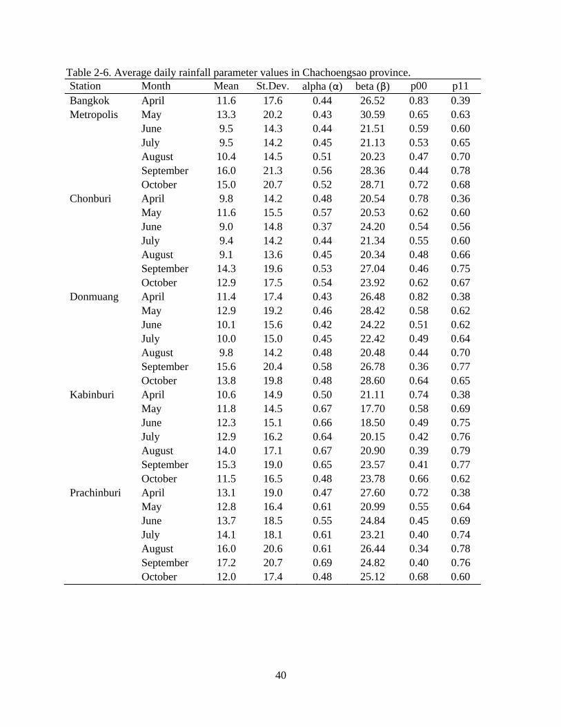
Table 2-6. Average daily rainfall parameter values in Chachoengsao province. Station Month Mean St.Dev. alpha (α) beta (β) p00 p11 Bangkok April 11.6 17.6 0.44 26.52 0.83 0.39 Metropolis May 13.3 20.2 0.43 30.59 0.65 0.63

June 9.5 14.3 0.44 21.51 0.59 0.60 July 9.5 14.2 0.45 21.13 0.53 0.65 August 10.4 14.5 0.51 20.23 0.47 0.70 September 16.0 21.3 0.56 28.36 0.44 0.78 October 15.0 20.7 0.52 28.71 0.72 0.68

Chonburi April 9.8 14.2 0.48 20.54 0.78 0.36 May 11.6 15.5 0.57 20.53 0.62 0.60 June 9.0 14.8 0.37 24.20 0.54 0.56 July 9.4 14.2 0.44 21.34 0.55 0.60 August 9.1 13.6 0.45 20.34 0.48 0.66 September 14.3 19.6 0.53 27.04 0.46 0.75 October 12.9 17.5 0.54 23.92 0.62 0.67

Donmuang April 11.4 17.4 0.43 26.48 0.82 0.38 May 12.9 19.2 0.46 28.42 0.58 0.62 June 10.1 15.6 0.42 24.22 0.51 0.62 July 10.0 15.0 0.45 22.42 0.49 0.64 August 9.8 14.2 0.48 20.48 0.44 0.70 September 15.6 20.4 0.58 26.78 0.36 0.77 October 13.8 19.8 0.48 28.60 0.64 0.65

Kabinburi April 10.6 14.9 0.50 21.11 0.74 0.38 May 11.8 14.5 0.67 17.70 0.58 0.69 June 12.3 15.1 0.66 18.50 0.49 0.75 July 12.9 16.2 0.64 20.15 0.42 0.76 August 14.0 17.1 0.67 20.90 0.39 0.79 September 15.3 19.0 0.65 23.57 0.41 0.77 October 11.5 16.5 0.48 23.78 0.66 0.62

Prachinburi April 13.1 19.0 0.47 27.60 0.72 0.38 May 12.8 16.4 0.61 20.99 0.55 0.64 June 13.7 18.5 0.55 24.84 0.45 0.69 July 14.1 18.1 0.61 23.21 0.40 0.74 August 16.0 20.6 0.61 26.44 0.34 0.78 September 17.2 20.7 0.69 24.82 0.40 0.76 October 12.0 17.4 0.48 25.12 0.68 0.60

40

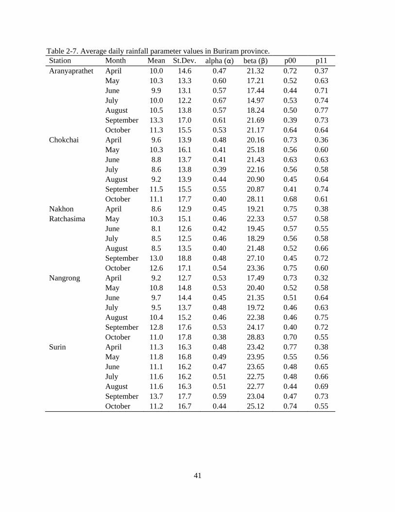
Table 2-7. Average daily rainfall parameter values in Buriram province. Station Month Mean St.Dev. alpha (α) beta (β) p00 p11 Aranyaprathet April 10.0 14.6 0.47 21.32 0.72 0.37


Chokchai April 9.6 13.9 0.48 20.16 0.73 0.36 May 10.3 16.1 0.41 25.18 0.56 0.60 June 8.8 13.7 0.41 21.43 0.63 0.63 July 8.6 13.8 0.39 22.16 0.56 0.58 August 9.2 13.9 0.44 20.90 0.45 0.64 September 11.5 15.5 0.55 20.87 0.41 0.74 October 11.1 17.7 0.40 28.11 0.68 0.61

Nakhon April 8.6 12.9 0.45 19.21 0.75 0.38 Ratchasima May 10.3 15.1 0.46 22.33 0.57 0.58

June 8.1 12.6 0.42 19.45 0.57 0.55 July 8.5 12.5 0.46 18.29 0.56 0.58 August 8.5 13.5 0.40 21.48 0.52 0.66 September 13.0 18.8 0.48 27.10 0.45 0.72 October 12.6 17.1 0.54 23.36 0.75 0.60

Nangrong April 9.2 12.7 0.53 17.49 0.73 0.32 May 10.8 14.8 0.53 20.40 0.52 0.58 June 9.7 14.4 0.45 21.35 0.51 0.64 July 9.5 13.7 0.48 19.72 0.46 0.63 August 10.4 15.2 0.46 22.38 0.46 0.75 September 12.8 17.6 0.53 24.17 0.40 0.72 October 11.0 17.8 0.38 28.83 0.70 0.55

Surin April 11.3 16.3 0.48 23.42 0.77 0.38 May 11.8 16.8 0.49 23.95 0.55 0.56 June 11.1 16.2 0.47 23.65 0.48 0.65 July 11.6 16.2 0.51 22.75 0.48 0.66 August 11.6 16.3 0.51 22.77 0.44 0.69 September 13.7 17.7 0.59 23.04 0.47 0.73 October 11.2 16.7 0.44 25.12 0.74 0.55

41

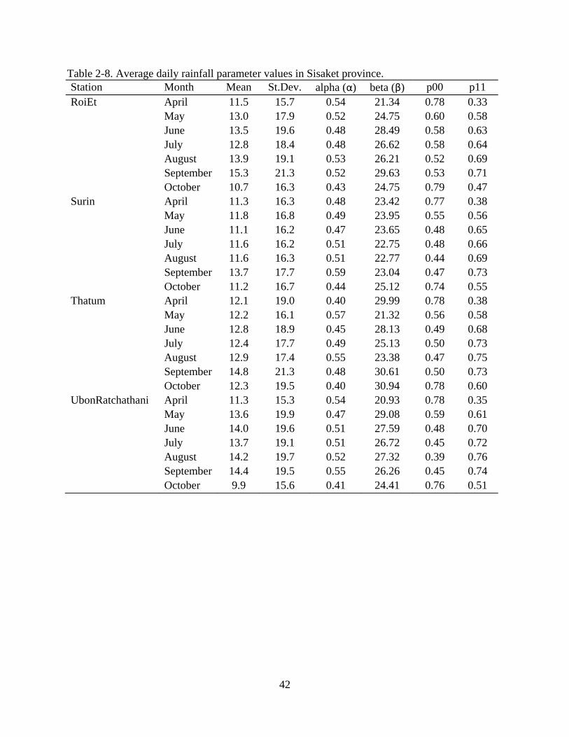
Table 2-8. Average daily rainfall parameter values in Sisaket province. Station Month Mean St.Dev. alpha (α) beta (β) p00 p11 RoiEt April 11.5 15.7 0.54 21.34 0.78 0.33


Surin April 11.3 16.3 0.48 23.42 0.77 0.38 May 11.8 16.8 0.49 23.95 0.55 0.56 June 11.1 16.2 0.47 23.65 0.48 0.65 July 11.6 16.2 0.51 22.75 0.48 0.66 August 11.6 16.3 0.51 22.77 0.44 0.69 September 13.7 17.7 0.59 23.04 0.47 0.73 October 11.2 16.7 0.44 25.12 0.74 0.55

Thatum April 12.1 19.0 0.40 29.99 0.78 0.38 May 12.2 16.1 0.57 21.32 0.56 0.58 June 12.8 18.9 0.45 28.13 0.49 0.68 July 12.4 17.7 0.49 25.13 0.50 0.73 August 12.9 17.4 0.55 23.38 0.47 0.75 September 14.8 21.3 0.48 30.61 0.50 0.73 October 12.3 19.5 0.40 30.94 0.78 0.60

UbonRatchathani April 11.3 15.3 0.54 20.93 0.78 0.35 May 13.6 19.9 0.47 29.08 0.59 0.61 June 14.0 19.6 0.51 27.59 0.48 0.70 July 13.7 19.1 0.51 26.72 0.45 0.72 August 14.2 19.7 0.52 27.32 0.39 0.76 September 14.4 19.5 0.55 26.26 0.45 0.74 October 9.9 15.6 0.41 24.41 0.76 0.51

42

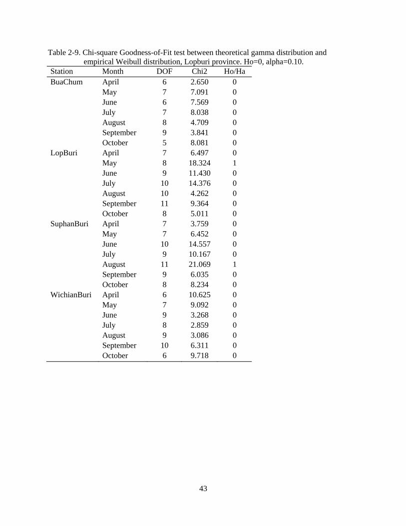
Table 2-9. Chi-square Goodness-of-Fit test between theoretical gamma distribution and empirical Weibull distribution, Lopburi province. Ho=0, alpha=0.10.

Station Month DOF Chi2 Ho/Ha BuaChum April 6 2.650 0

May 7 7.091 0 June 6 7.569 0 July 7 8.038 0 August 8 4.709 0 September 9 3.841 0 October 5 8.081 0

LopBuri April 7 6.497 0 May 8 18.324 1 June 9 11.430 0 July 10 14.376 0 August 10 4.262 0 September 11 9.364 0 October 8 5.011 0

SuphanBuri April 7 3.759 0 May 7 6.452 0 June 10 14.557 0 July 9 10.167 0 August 11 21.069 1 September 9 6.035 0 October 8 8.234 0

WichianBuri April 6 10.625 0 May 7 9.092 0 June 9 3.268 0 July 8 2.859 0 August 9 3.086 0 September 10 6.311 0 October 6 9.718 0

43

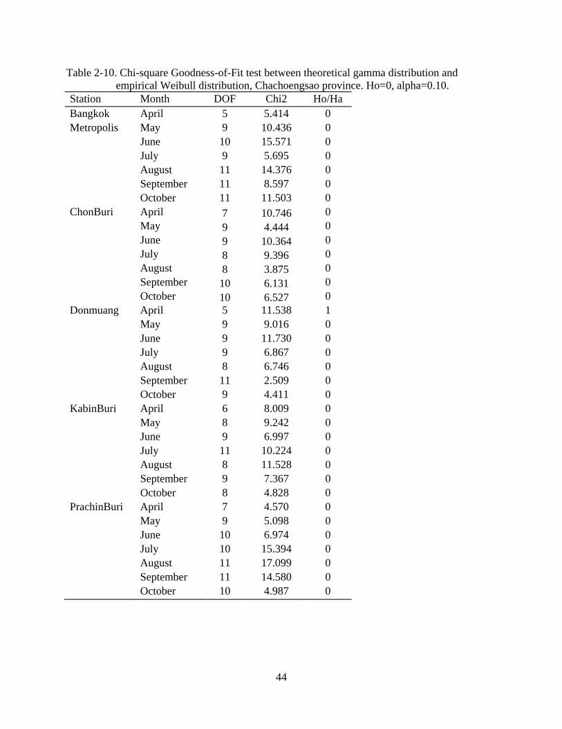
Table 2-10. Chi-square Goodness-of-Fit test between theoretical gamma distribution and empirical Weibull distribution, Chachoengsao province. Ho=0, alpha=0.10.

Station Month DOF Chi2 Ho/Ha Bangkok April 5 5.414 0 Metropolis May 9 10.436 0

June 10 15.571 0 July 9 5.695 0 August 11 14.376 0 September 11 8.597 0 October 11 11.503 0

ChonBuri April 7 10.746 0 May 9 4.444 0 June 9 10.364 0 July 8 9.396 0 August 8 3.875 0 September 10 6.131 0 October 10 6.527 0

Donmuang April 5 11.538 1 May 9 9.016 0 June 9 11.730 0 July 9 6.867 0 August 8 6.746 0 September 11 2.509 0 October 9 4.411 0

KabinBuri April 6 8.009 0 May 8 9.242 0 June 9 6.997 0 July 11 10.224 0 August 8 11.528 0 September 9 7.367 0 October 8 4.828 0

PrachinBuri April 7 4.570 0 May 9 5.098 0 June 10 6.974 0 July 10 15.394 0 August 11 17.099 0 September 11 14.580 0 October 10 4.987 0

44

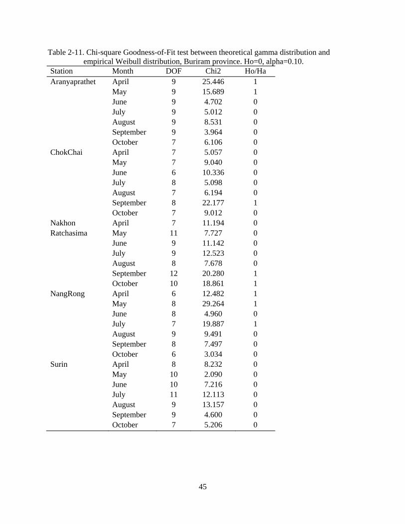
Table 2-11. Chi-square Goodness-of-Fit test between theoretical gamma distribution and empirical Weibull distribution, Buriram province. Ho=0, alpha=0.10.

Station Month DOF Chi2 Ho/Ha Aranyaprathet April 9 25.446 1


ChokChai April 7 5.057 0 May 7 9.040 0 June 6 10.336 0 July 8 5.098 0 August 7 6.194 0 September 8 22.177 1 October 7 9.012 0

Nakhon April 7 11.194 0 Ratchasima May 11 7.727 0


NangRong April 6 12.482 1 May 8 29.264 1 June 8 4.960 0 July 7 19.887 1 August 9 9.491 0 September 8 7.497 0 October 6 3.034 0

Surin April 8 8.232 0 May 10 2.090 0 June 10 7.216 0 July 11 12.113 0 August 9 13.157 0 September 9 4.600 0 October 7 5.206 0

45

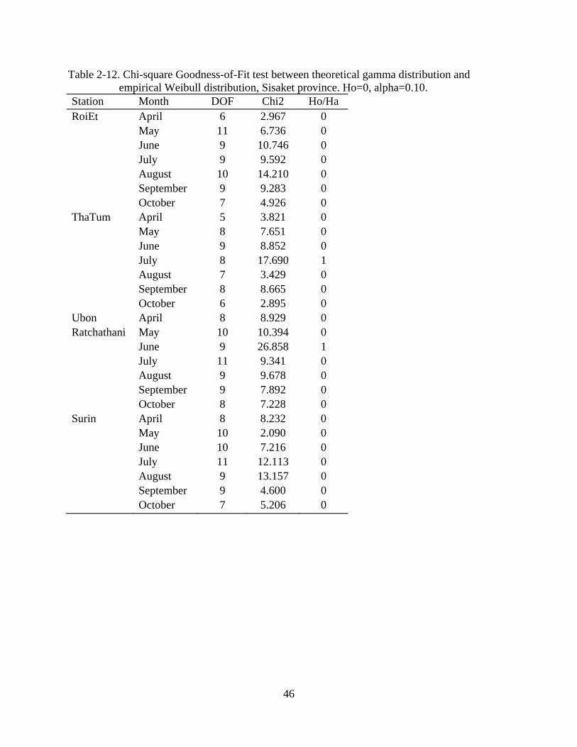
Table 2-12. Chi-square Goodness-of-Fit test between theoretical gamma distribution and empirical Weibull distribution, Sisaket province. Ho=0, alpha=0.10.

Station Month DOF Chi2 Ho/Ha RoiEt April 6 2.967 0


ThaTum April 5 3.821 0 May 8 7.651 0 June 9 8.852 0 July 8 17.690 1 August 7 3.429 0 September 8 8.665 0 October 6 2.895 0

Ubon April 8 8.929 0 Ratchathani May 10 10.394 0


Surin April 8 8.232 0 May 10 2.090 0 June 10 7.216 0 July 11 12.113 0 August 9 13.157 0 September 9 4.600 0 October 7 5.206 0

46

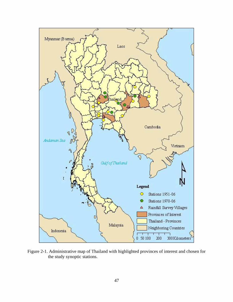
Figure 2-1. Administrative map of Thailand with highlighted provinces of interest and chosen for the study synoptic stations.

47

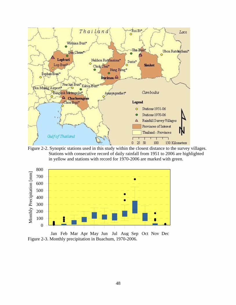
Figure 2-2. Synoptic stations used in this study within the closest distance to the survey villages.

Stations with consecutive record of daily rainfall from 1951 to 2006 are highlighted in yellow and stations with record for 1970-2006 are marked with green.

0

200

400

600

800

100

300

500

700

Mon

thly

Pre

cipi

tatio

n [m

m]

Jan Feb Mar Apr May Jun Jul Aug Sep Oct Nov Dec Figure 2-3. Monthly precipitation in Buachum, 1970-2006.

48

0

200

400

600

800

100

300

500

700M

onth

ly P

reci

pita

tion

[mm

]

Jan Feb Mar Apr May Jun Jul Aug Sep Oct Nov Dec Figure 2-4. Monthly precipitation in Lopburi, 1951-2006.

0

200

400

600

800

100

300

500

700

Mon

thly

Pre

cipi

tatio

n [m

m]

Jan Feb Mar Apr May Jun Jul Aug Sep Oct Nov Dec Figure 2-5. Monthly precipitation in Suphanburi, 1951-2006.

0

200

400

600

800

100

300

500

700

Mon

thly

Pre

cipi

tatio

n [m

m]

Jan Feb Mar Apr May Jun Jul Aug Sep Oct Nov Dec Figure 2-6. Monthly precipitation in Wichianburi, 1970-2006.

49

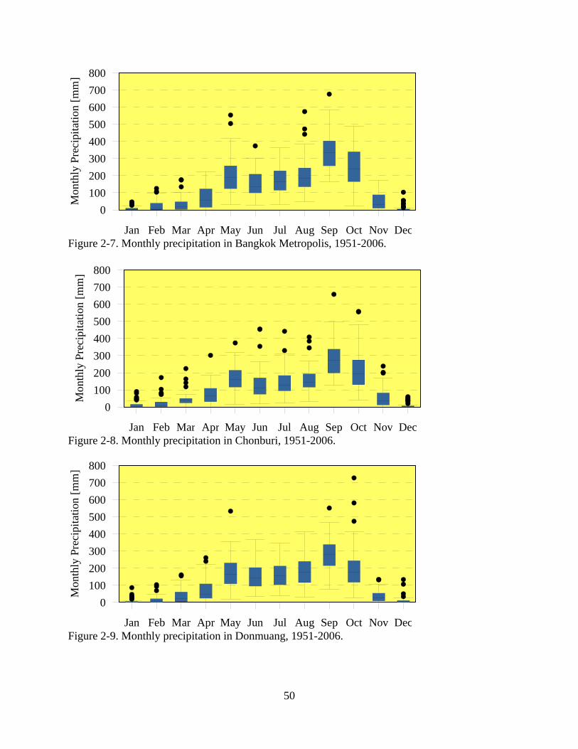
0

200

400

600

800

100

300

500

700M

onth

ly P

reci

pita

tion

[mm

]

Jan Feb Mar Apr May Jun Jul Aug Sep Oct Nov Dec Figure 2-7. Monthly precipitation in Bangkok Metropolis, 1951-2006.

0

200

400

600

800

100

300

500

700

Mon

thly

Pre

cipi

tatio

n [m

m]

Jan Feb Mar Apr May Jun Jul Aug Sep Oct Nov Dec Figure 2-8. Monthly precipitation in Chonburi, 1951-2006.

0

200

400

600

800

100

300

500

700

Mon

thly

Pre

cipi

tatio

n [m

m]

Jan Feb Mar Apr May Jun Jul Aug Sep Oct Nov Dec Figure 2-9. Monthly precipitation in Donmuang, 1951-2006.

50

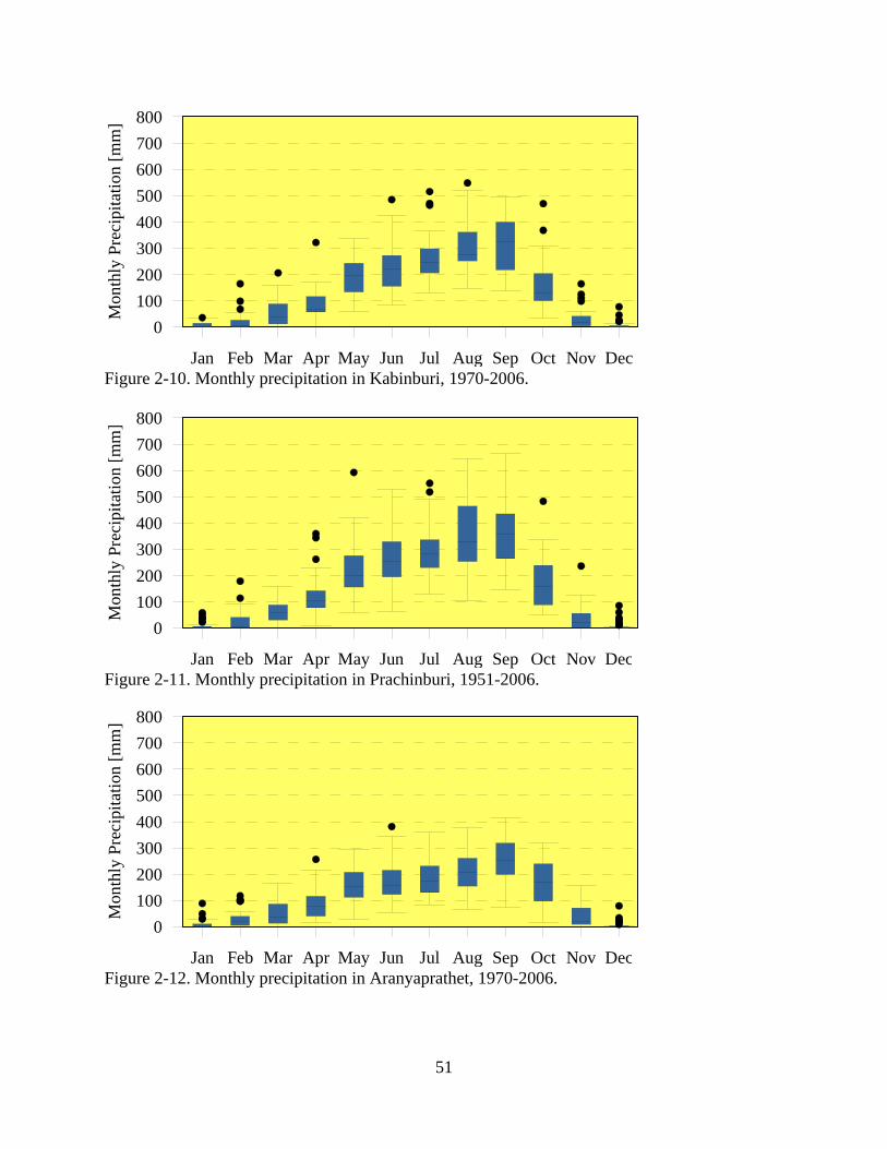
0

200

400

600

800

100

300

500

700

Mon

thly

Pre

cipi

tatio

n [m

m]

Jan Feb Mar Apr May Jun Jul Aug Sep Oct Nov Dec Figure 2-10. Monthly precipitation in Kabinburi, 1970-2006.

0

200

400

600

800

100

300

500

700

Mon

thly

Pre

cipi

tatio

n [m

m]

Jan Feb Mar Apr May Jun Jul Aug Sep Oct Nov Dec Figure 2-11. Monthly precipitation in Prachinburi, 1951-2006.

0

200

400

600

800

100

300

500

700

Mon

thly

Pre

cipi

tatio

n [m

m]

Jan Feb Mar Apr May Jun Jul Aug Sep Oct Nov Dec Figure 2-12. Monthly precipitation in Aranyaprathet, 1970-2006.

51

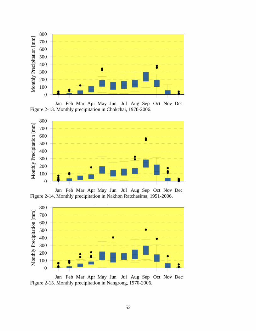
0

200

400

600

800

100

300

500

700

Mon

thly

Pre

cipi

tatio

n [m

m]

Jan Feb Mar Apr May Jun Jul Aug Sep Oct Nov Dec Figure 2-13. Monthly precipitation in Chokchai, 1970-2006.

0

200

400

600

800

100

300

500

700

Mon

thly

Pre

cipi

tatio

n [m

m]

Jan Feb Mar Apr May Jun Jul Aug Sep Oct Nov Dec Figure 2-14. Monthly precipitation in Nakhon Ratchasima, 1951-2006.

0

200

400

600

800

100

300

500

700

Mon

thly

Pre

cipi

tatio

n [m

m]

Jan Feb Mar Apr May Jun Jul Aug Sep Oct Nov Dec

g g

Figure 2-15. Monthly precipitation in Nangrong, 1970-2006.

52

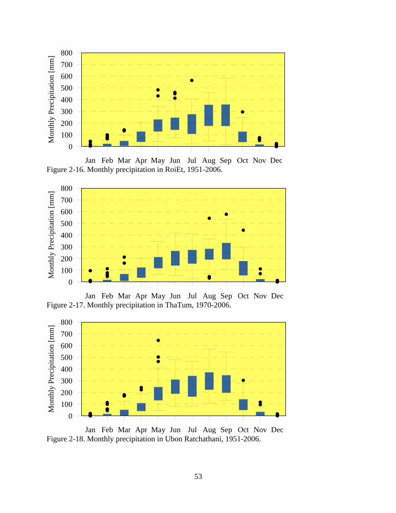
0

200

400

600

800

100

300

500

700

Mon

thly

Pre

cipi

tatio

n [m

m]

Jan Feb Mar Apr May Jun Jul Aug Sep Oct Nov Dec Figure 2-16. Monthly precipitation in RoiEt, 1951-2006.

0

200

400

600

800

100

300

500

700

Mon

thly

Pre

cipi

tatio

n [m

m]

Jan Feb Mar Apr May Jun Jul Aug Sep Oct Nov Dec Figure 2-17. Monthly precipitation in ThaTum, 1970-2006.

0

200

400

600

800

100

300

500

700

Mon

thly

Pre

cipi

tatio

n [m

m]

Jan Feb Mar Apr May Jun Jul Aug Sep Oct Nov Dec Figure 2-18. Monthly precipitation in Ubon Ratchathani, 1951-2006.

53

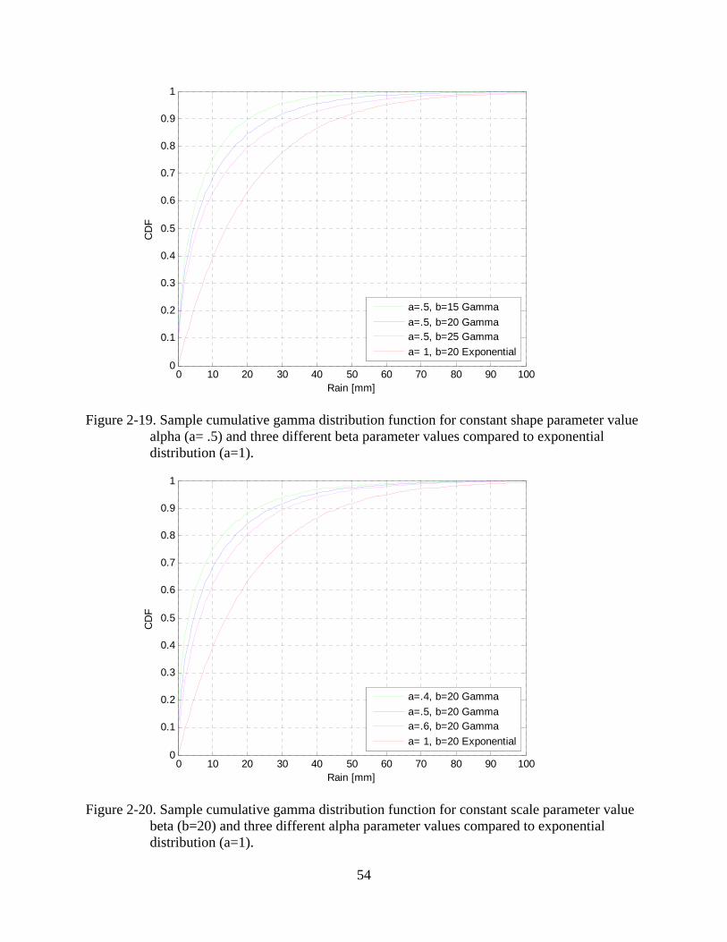
0 10 20 30 40 50 60 70 80 90 1000

0.1

0.2

0.3

0.4

0.5

0.6

0.7

0.8

0.9

1

Rain [mm]

CD

F

a=.5, b=15 Gammaa=.5, b=20 Gammaa=.5, b=25 Gammaa= 1, b=20 Exponential

Figure 2-19. Sample cumulative gamma distribution function for constant shape parameter value alpha (a= .5) and three different beta parameter values compared to exponential distribution (a=1).

0 10 20 30 40 50 60 70 80 90 1000

0.1

0.2

0.3

0.4

0.5

0.6

0.7

0.8

0.9

1

Rain [mm]

CD

F

a=.4, b=20 Gammaa=.5, b=20 Gammaa=.6, b=20 Gammaa= 1, b=20 Exponential

Figure 2-20. Sample cumulative gamma distribution function for constant scale parameter value beta (b=20) and three different alpha parameter values compared to exponential distribution (a=1).

54

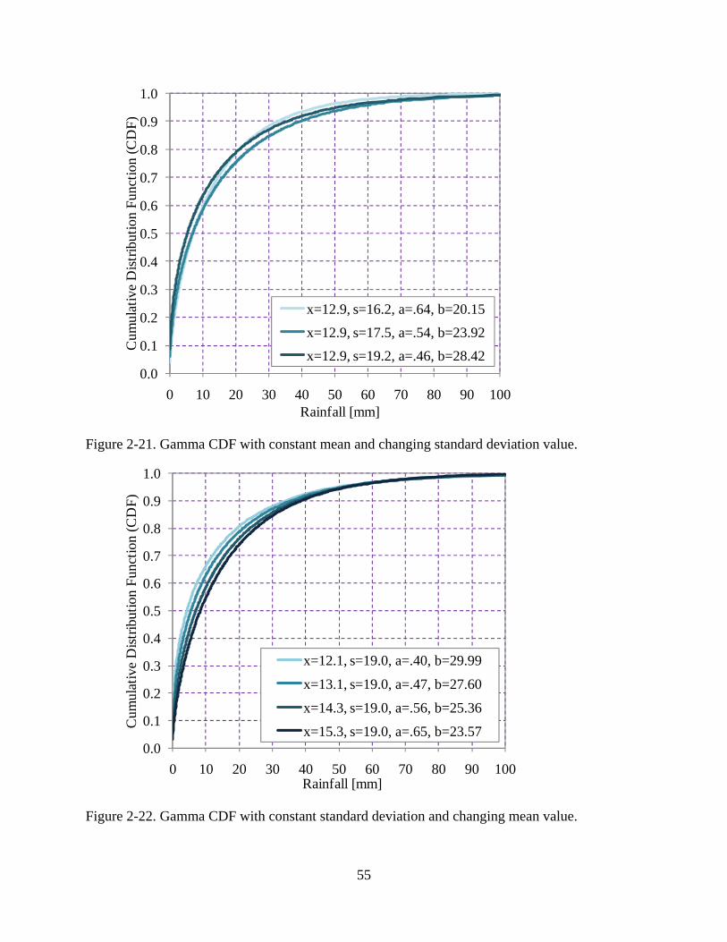
0.0

0.1

0.2

0.3

0.4

0.5

0.6

0.7

0.8

0.9

1.0

0 10 20 30 40 50 60 70 80 90 100

Cum

ulat

ive

Dist

ribut

ion

Func

tion

(CD

F)

Rainfall [mm]

x=12.9, s=16.2, a=.64, b=20.15

x=12.9, s=17.5, a=.54, b=23.92x=12.9, s=19.2, a=.46, b=28.42

Figure 2-21. Gamma CDF with constant mean and changing standard deviation value.

0.0

0.1

0.2

0.3

0.4

0.5

0.6

0.7

0.8

0.9

1.0

0 10 20 30 40 50 60 70 80 90 100

Cum

ulat

ive

Dist

ribut

ion

Func

tion

(CD

F)

Rainfall [mm]

x=12.1, s=19.0, a=.40, b=29.99

x=13.1, s=19.0, a=.47, b=27.60

x=14.3, s=19.0, a=.56, b=25.36

x=15.3, s=19.0, a=.65, b=23.57

Figure 2-22. Gamma CDF with constant standard deviation and changing mean value.

55

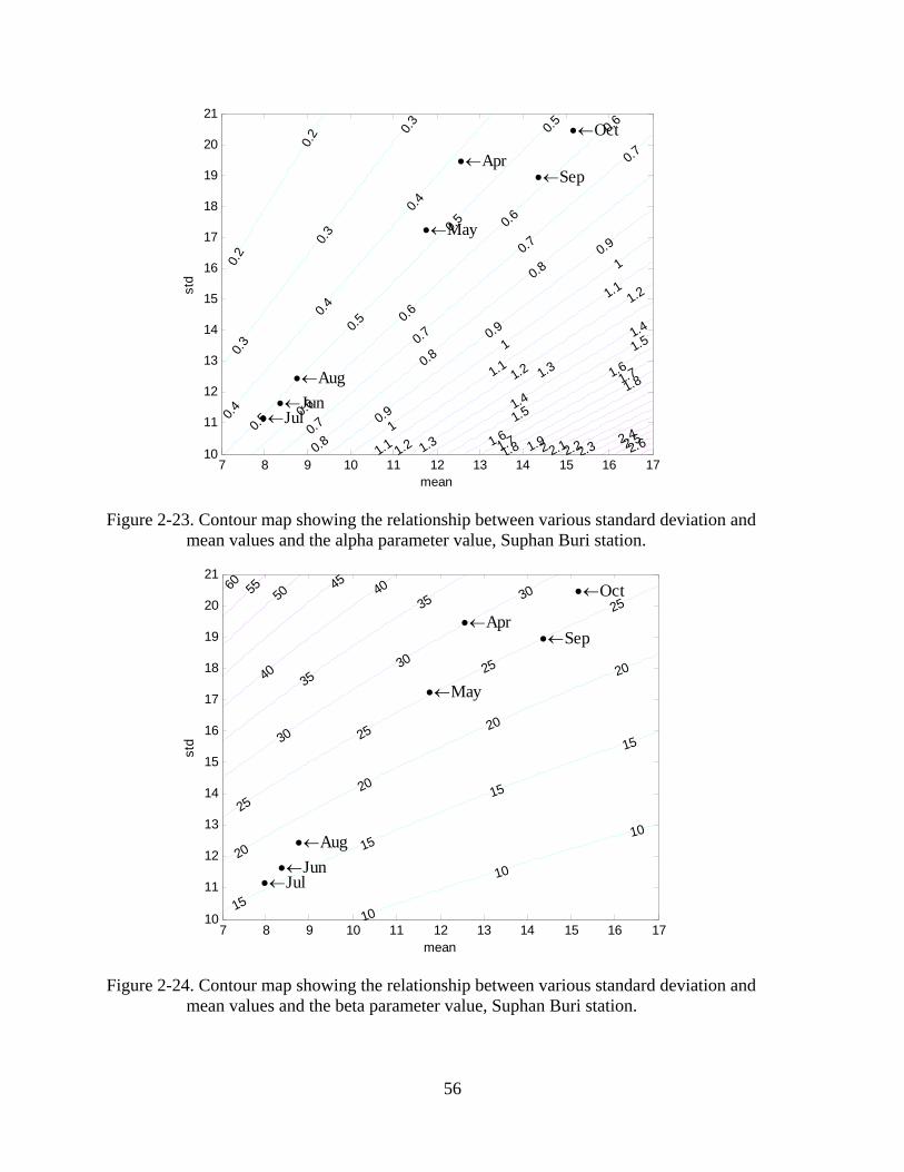
0.2

0.2

0.3

0.3

0.3

0.4

0.4

0.4

0.5

0.5

0.5

0.5

0.6

0.6

0.6

0.6

0.7

0.7

0.7

0.7

0.8

0.8

0.8

0.9

0.9

0.9

1

1

1

1.1

1.1

1.1

1.2

1.2

1.2

1.3

1.3

1.4

1.4

1.5

1.5

1.6

1.6

1.7

1.7

1.8

1.8

1.92 2.12.22.32.42.52.6

mean

std

•←Apr

•←May

•←Jun•←Jul

•←Aug

•←Sep

•←Oct

7 8 9 10 11 12 13 14 15 16 1710

11

12

13

14

15

16

17

18

19

20

21

Figure 2-23. Contour map showing the relationship between various standard deviation and mean values and the alpha parameter value, Suphan Buri station.

10

10

10

15

15

15

15

20

20

20

20

25

25

25

2530

30

30

35

35

40

40

45505560

mean

std

•←Apr

•←May

•←Jun•←Jul

•←Aug

•←Sep

•←Oct

7 8 9 10 11 12 13 14 15 16 1710

11

12

13

14

15

16

17

18

19

20

21

Figure 2-24. Contour map showing the relationship between various standard deviation and mean values and the beta parameter value, Suphan Buri station.

56

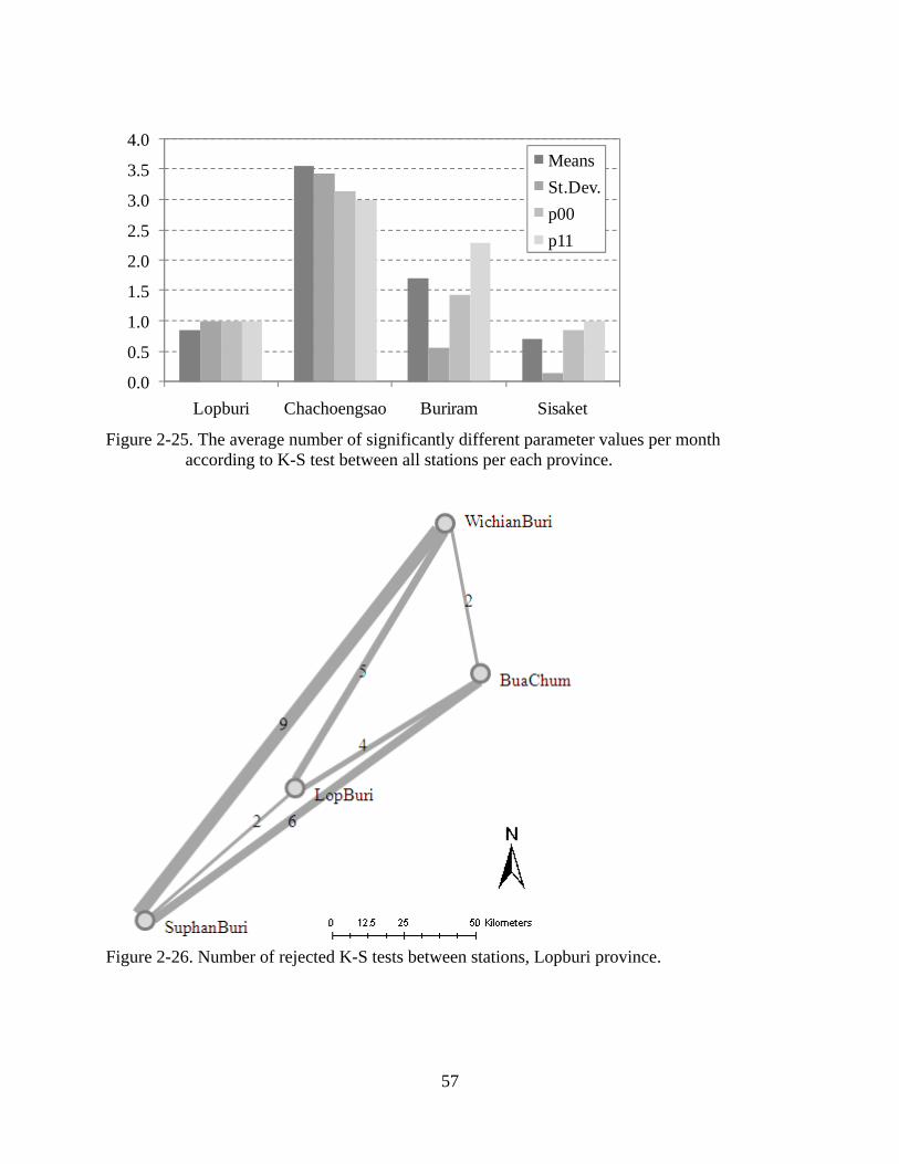
0.0

0.5

1.0

1.5

2.0

2.5

3.0

3.5

4.0

Lopburi Chachoengsao Buriram Sisaket

MeansSt.Dev.p00p11

Figure 2-25. The average number of significantly different parameter values per month

according to K-S test between all stations per each province.

Figure 2-26. Number of rejected K-S tests between stations, Lopburi province.

57

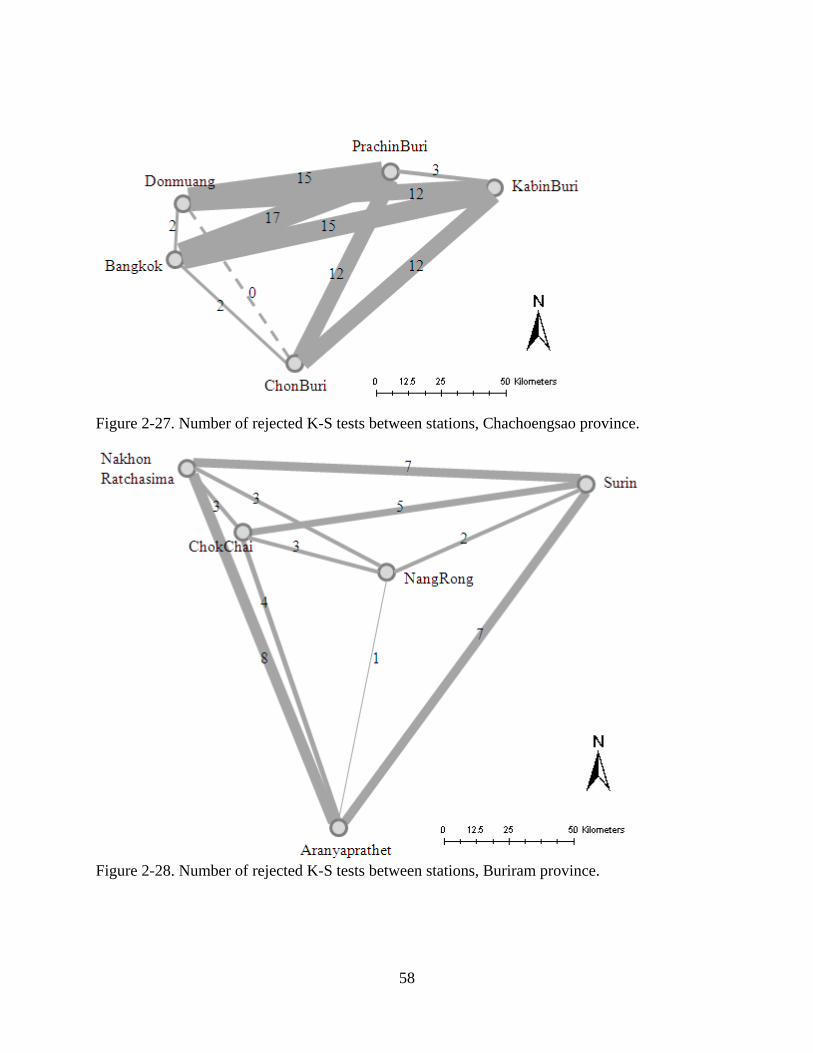
Figure 2-27. Number of rejected K-S tests between stations, Chachoengsao province.

Figure 2-28. Number of rejected K-S tests between stations, Buriram province.

58

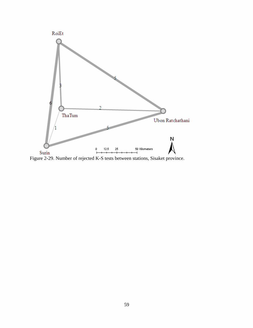
Figure 2-29. Number of rejected K-S tests between stations, Sisaket province.

59

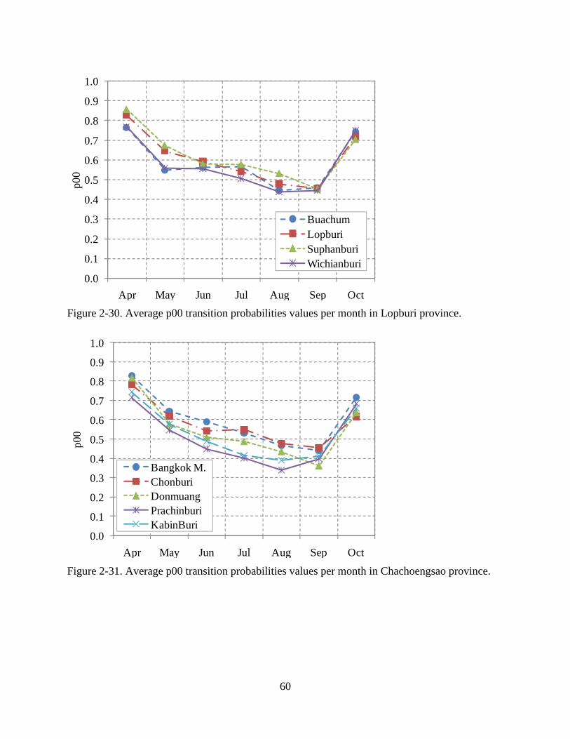
0.0

0.1

0.2

0.3

0.4

0.5

0.6

0.7

0.8

0.9

1.0

Apr May Jun Jul Aug Sep Oct

p00

BuachumLopburiSuphanburiWichianburi

Figure 2-30. Average p00 transition probabilities values per month in Lopburi province.

0.0

0.1

0.2

0.3

0.4

0.5

0.6

0.7

0.8

0.9

1.0


p00

Bangkok M.ChonburiDonmuangPrachinburiKabinBuri

Figure 2-31. Average p00 transition probabilities values per month in Chachoengsao province.

60

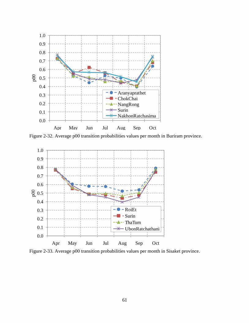
0.0

0.1

0.2

0.3

0.4

0.5

0.6

0.7

0.8

0.9

1.0


p00

AranyaprathetChokChaiNangRongSurinNakhonRatchasima

Figure 2-32. Average p00 transition probabilities values per month in Buriram province.

0.0

0.1

0.2

0.3

0.4

0.5

0.6

0.7

0.8

0.9

1.0


p00

RoiEtSurinThaTumUbonRatchathani

Figure 2-33. Average p00 transition probabilities values per month in Sisaket province.

61

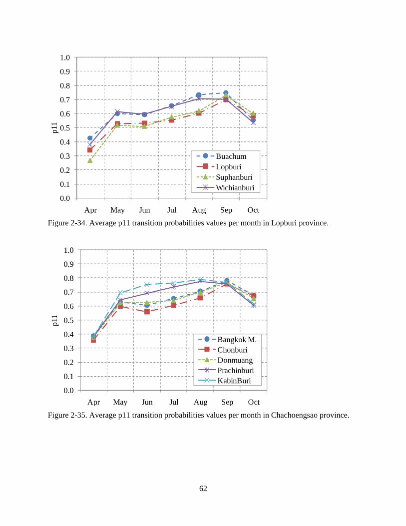
0.0

0.1

0.2

0.3

0.4

0.5

0.6

0.7

0.8

0.9

1.0


p11


Figure 2-34. Average p11 transition probabilities values per month in Lopburi province.

0.0

0.1

0.2

0.3

0.4

0.5

0.6

0.7

0.8

0.9

1.0


p11


Figure 2-35. Average p11 transition probabilities values per month in Chachoengsao province.

62

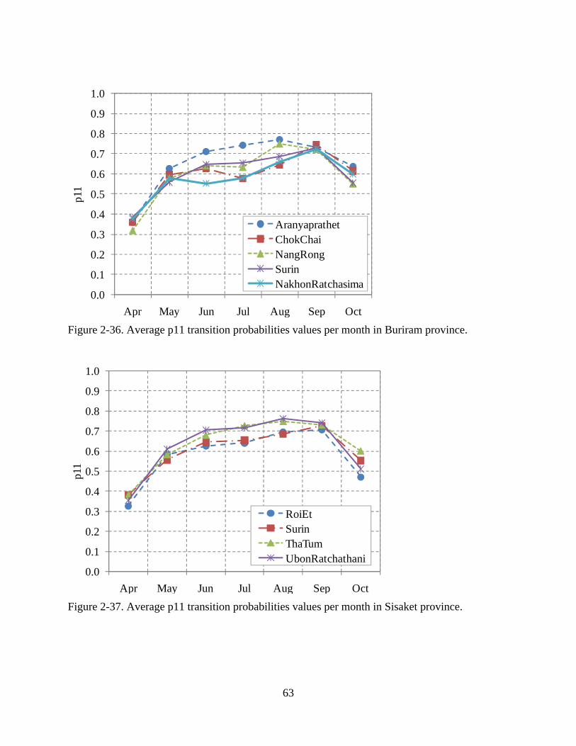
0.0

0.1

0.2

0.3

0.4

0.5

0.6

0.7

0.8

0.9

1.0


p11


Figure 2-36. Average p11 transition probabilities values per month in Buriram province.

0.0

0.1

0.2

0.3

0.4

0.5

0.6

0.7

0.8

0.9

1.0


p11


Figure 2-37. Average p11 transition probabilities values per month in Sisaket province.

63

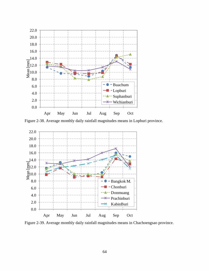
0.0

2.0

4.0

6.0

8.0

10.0

12.0

14.0

16.0

18.0

20.0

22.0


Mea

n [m

m]


Figure 2-38. Average monthly daily rainfall magnitudes means in Lopburi province.

0.0

2.0

4.0

6.0

8.0

10.0

12.0

14.0

16.0

18.0

20.0

22.0


Mea

n [m

m]


Figure 2-39. Average monthly daily rainfall magnitudes means in Chachoengsao province.

64

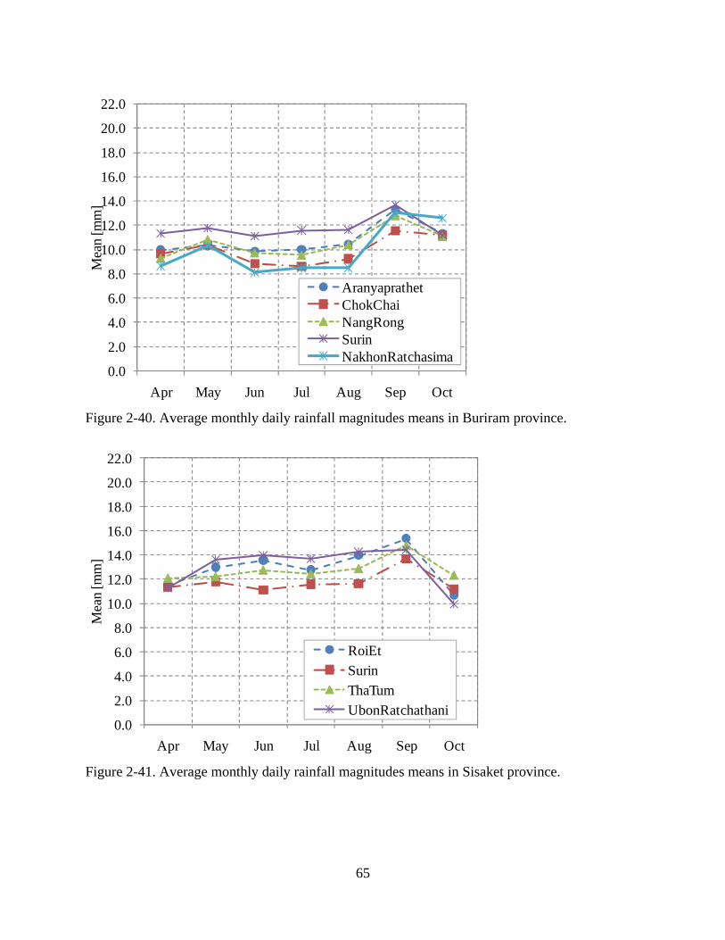
0.0

2.0

4.0

6.0

8.0

10.0

12.0

14.0

16.0

18.0

20.0

22.0


Mea

n [m

m]


Figure 2-40. Average monthly daily rainfall magnitudes means in Buriram province.

0.0

2.0

4.0

6.0

8.0

10.0

12.0

14.0

16.0

18.0

20.0

22.0


Mea

n [m

m]


Figure 2-41. Average monthly daily rainfall magnitudes means in Sisaket province.

65

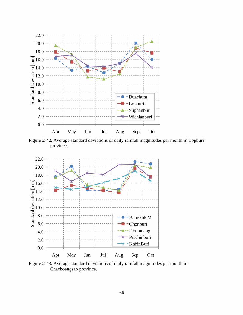
0.0

2.0

4.0

6.0

8.0

10.0

12.0

14.0

16.0

18.0

20.0

22.0


Stan

dard

Dev

iatio

n [m

m]


Figure 2-42. Average standard deviations of daily rainfall magnitudes per month in Lopburi

province.

0.0

2.0

4.0

6.0

8.0

10.0

12.0

14.0

16.0

18.0

20.0

22.0


Stan

dard

dev

iatio

n [m

m]


Figure 2-43. Average standard deviations of daily rainfall magnitudes per month in

Chachoengsao province.

66

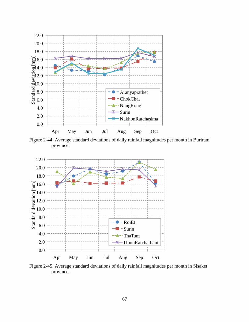
0.0

2.0

4.0

6.0

8.0

10.0

12.0

14.0

16.0

18.0

20.0

22.0


Stan

dard

dev

iatio

n [m

m]


Figure 2-44. Average standard deviations of daily rainfall magnitudes per month in Buriram

province.

0.0

2.0

4.0

6.0

8.0

10.0

12.0

14.0

16.0

18.0

20.0

22.0


Stan

dard

dev

aitio

n [m

m]


Figure 2-45. Average standard deviations of daily rainfall magnitudes per month in Sisaket

province.

67

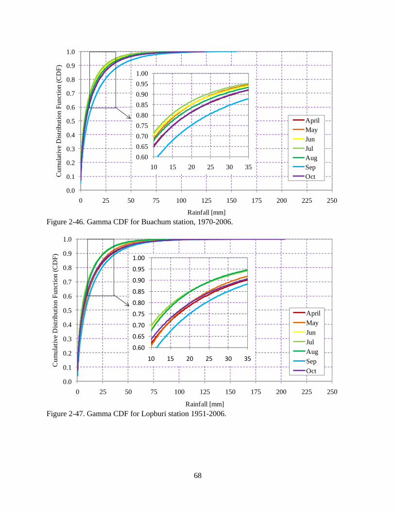
0.0

0.1

0.2

0.3

0.4

0.5

0.6

0.7

0.8

0.9

1.0

0 25 50 75 100 125 150 175 200 225 250

Cum

ulat

ive

Dist

ribut

ion

Func

tion

(CD

F)

Rainfall [mm]

AprilMayJunJulAugSepOct

0.600.650.700.750.800.850.900.951.00

10 15 20 25 30 35

Figure 2-46. Gamma CDF for Buachum station, 1970-2006.

0.0

0.1

0.2

0.3

0.4

0.5

0.6

0.7

0.8

0.9

1.0

0 25 50 75 100 125 150 175 200 225 250

Cum

ulat

ive

Dist

ribut

ion

Func

tion

(CD

F)

Rainfall [mm]


0.60

0.65

0.70

0.75

0.80

0.85

0.90

0.95

1.00

10 15 20 25 30 35

Figure 2-47. Gamma CDF for Lopburi station 1951-2006.

68

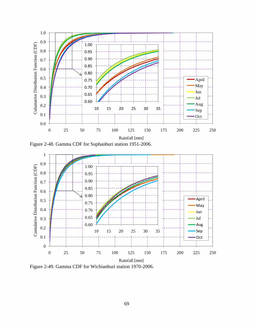
0.0

0.1

0.2

0.3

0.4

0.5

0.6

0.7

0.8

0.9

1.0

0 25 50 75 100 125 150 175 200 225 250

Cul

umat

ive

Dist

ribut

ion

Func

tion

(CD

F)

Rainfall [mm]


0.60

0.65

0.70

0.75

0.80

0.85

0.90

0.95

1.00

10 15 20 25 30 35

Figure 2-48. Gamma CDF for Suphanburi station 1951-2006.

0

0.1

0.2

0.3

0.4

0.5

0.6

0.7

0.8

0.9

1

0 25 50 75 100 125 150 175 200 225 250

Cum

ulat

ive

Dist

ribut

ion

Func

tion

(CD

F)

Rainfall [mm]

April

May

Jun

Jul

Aug

Sep

Oct

0.60

0.65

0.70

0.75

0.80

0.85

0.90

0.95

1.00

10 15 20 25 30 35

Figure 2-49. Gamma CDF for Wichianburi station 1970-2006.

69

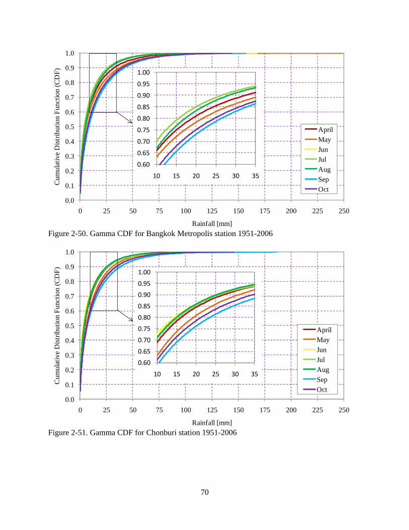
0.0

0.1

0.2

0.3

0.4

0.5

0.6

0.7

0.8

0.9

1.0

0 25 50 75 100 125 150 175 200 225 250

Cum

ulat

ive

Dist

ribut

ion

Func

tion

(CD

F)

Rainfall [mm]


0.60

0.65

0.70

0.75

0.80

0.85

0.90

0.95

1.00

10 15 20 25 30 35

Figure 2-50. Gamma CDF for Bangkok Metropolis station 1951-2006

0.0

0.1

0.2

0.3

0.4

0.5

0.6

0.7

0.8

0.9

1.0

0 25 50 75 100 125 150 175 200 225 250

Cum

ulat

ive

Dist

ribut

ion

Func

tion

(CD

F)

Rainfall [mm]


0.60

0.65

0.70

0.75

0.80

0.85

0.90

0.95

1.00

10 15 20 25 30 35

Figure 2-51. Gamma CDF for Chonburi station 1951-2006

70

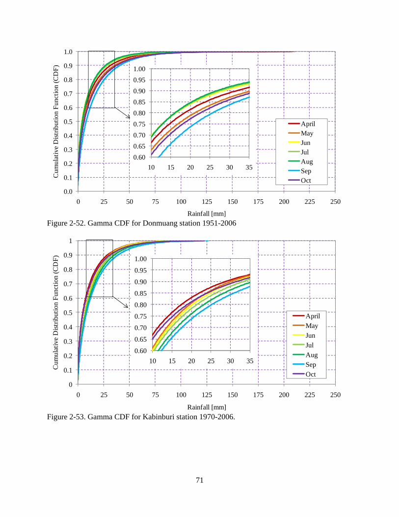
0.0

0.1

0.2

0.3

0.4

0.5

0.6

0.7

0.8

0.9

1.0

0 25 50 75 100 125 150 175 200 225 250

Cum

ulat

ive

Dist

ribut

ion

Func

tion

(CD

F)

Rainfall [mm]


0.600.650.700.750.800.850.900.951.00

10 15 20 25 30 35

Figure 2-52. Gamma CDF for Donmuang station 1951-2006

0

0.1

0.2

0.3

0.4

0.5

0.6

0.7

0.8

0.9

1

0 25 50 75 100 125 150 175 200 225 250

Cum

ulat

ive

Dist

ribut

ion

Func

tion

(CD

F)

Rainfall [mm]


0.60

0.65

0.70

0.75

0.80

0.85

0.90

0.95

1.00

10 15 20 25 30 35

Figure 2-53. Gamma CDF for Kabinburi station 1970-2006.

71

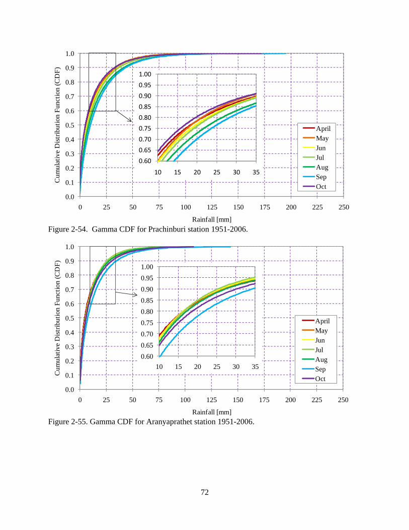
0.0

0.1

0.2

0.3

0.4

0.5

0.6

0.7

0.8

0.9

1.0

0 25 50 75 100 125 150 175 200 225 250

Cum

ulat

ive

Dist

ribut

ion

Func

tion

(CD

F)

Rainfall [mm]


0.60

0.65

0.70

0.75

0.80

0.85

0.90

0.95

1.00

10 15 20 25 30 35

Figure 2-54. Gamma CDF for Prachinburi station 1951-2006.

0.0

0.1

0.2

0.3

0.4

0.5

0.6

0.7

0.8

0.9

1.0

0 25 50 75 100 125 150 175 200 225 250

Cum

ulat

ive

Dist

ribut

ion

Func

tion

(CD

F)

Rainfall [mm]


0.600.650.700.750.800.850.900.951.00

10 15 20 25 30 35

Figure 2-55. Gamma CDF for Aranyaprathet station 1951-2006.

72

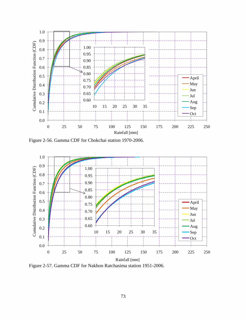
0.0

0.1

0.2

0.3

0.4

0.5

0.6

0.7

0.8

0.9

1.0

0 25 50 75 100 125 150 175 200 225 250

Cum

ulat

ive

Dist

ribut

ion

Func

tion

(CD

F)

Rainfall [mm]


0.600.650.700.750.800.850.900.951.00

10 15 20 25 30 35

Figure 2-56. Gamma CDF for Chokchai station 1970-2006.

0.0

0.1

0.2

0.3

0.4

0.5

0.6

0.7

0.8

0.9

1.0

0 25 50 75 100 125 150 175 200 225 250

Cum

ulat

ive

Dist

ribut

ion

Func

tion

(CD

F)

Rainfall [mm]


0.60

0.65

0.70

0.75

0.80

0.85

0.90

0.95

1.00

10 15 20 25 30 35

Figure 2-57. Gamma CDF for Nakhon Ratchasima station 1951-2006.

73

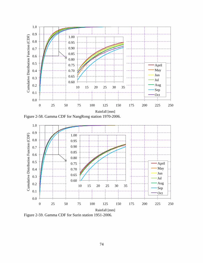
0.0

0.1

0.2

0.3

0.4

0.5

0.6

0.7

0.8

0.9

1.0

0 25 50 75 100 125 150 175 200 225 250

Cum

ulat

ive

Dist

ribut

ion

Func

tion

(CD

F)

Rainfall [mm]


0.600.650.700.750.800.850.900.951.00

10 15 20 25 30 35

Figure 2-58. Gamma CDF for NangRong station 1970-2006.

0.0

0.1

0.2

0.3

0.4

0.5

0.6

0.7

0.8

0.9

1.0

0 25 50 75 100 125 150 175 200 225 250

Cum

ulat

ive

Dist

ribut

ion

Func

tion

(CD

F)

Rainfall [mm]


0.600.650.700.750.800.850.900.951.00

10 15 20 25 30 35

Figure 2-59. Gamma CDF for Surin station 1951-2006.

74

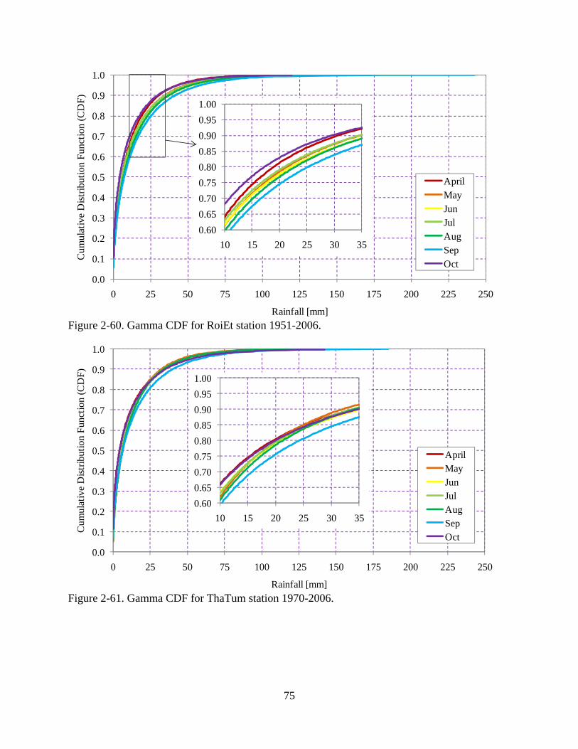
0.0

0.1

0.2

0.3

0.4

0.5

0.6

0.7

0.8

0.9

1.0

0 25 50 75 100 125 150 175 200 225 250

Cum

ulat

ive

Dist

ribut

ion

Func

tion

(CD

F)

Rainfall [mm]


0.600.650.700.750.800.850.900.951.00

10 15 20 25 30 35

Figure 2-60. Gamma CDF for RoiEt station 1951-2006.

0.0

0.1

0.2

0.3

0.4

0.5

0.6

0.7

0.8

0.9

1.0

0 25 50 75 100 125 150 175 200 225 250

Cum

ulat

ive

Dist

ribut

ion

Func

tion

(CD

F)

Rainfall [mm]


0.600.650.700.750.800.850.900.951.00

10 15 20 25 30 35

Figure 2-61. Gamma CDF for ThaTum station 1970-2006.

75

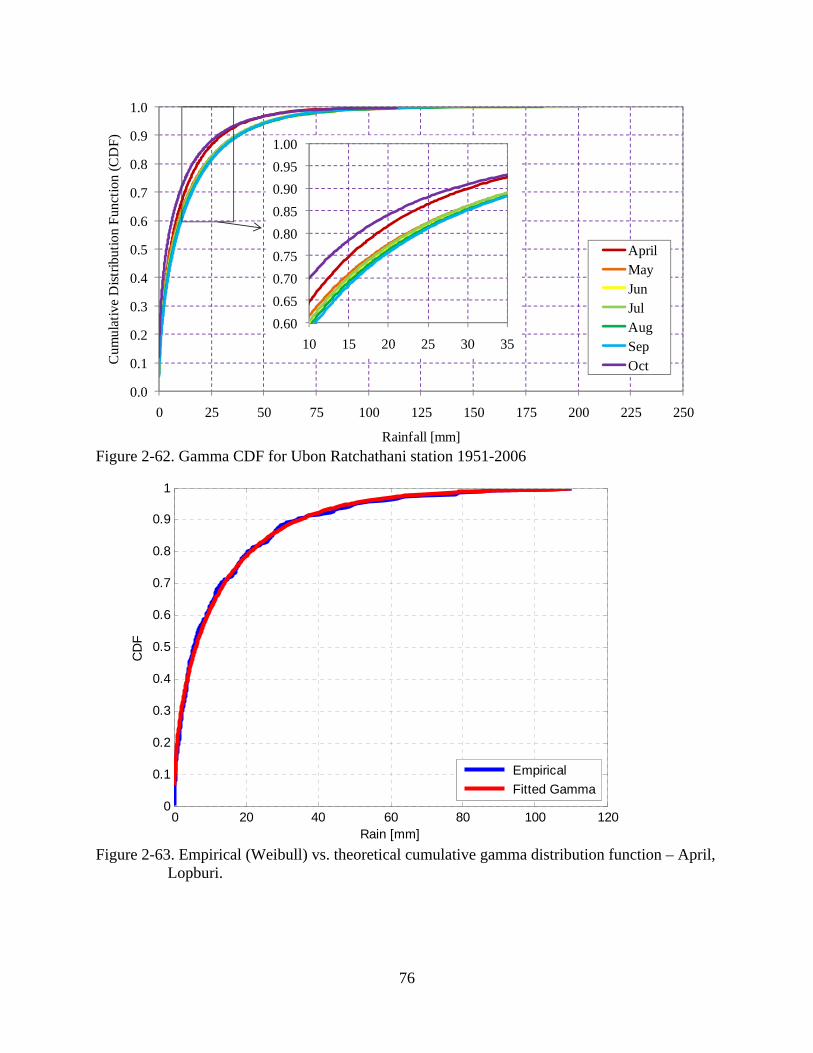
0.0

0.1

0.2

0.3

0.4

0.5

0.6

0.7

0.8

0.9

1.0

0 25 50 75 100 125 150 175 200 225 250

Cum

ulat

ive

Dist

ribut

ion

Func

tion

(CD

F)

Rainfall [mm]


0.600.650.700.750.800.850.900.951.00

10 15 20 25 30 35

Figure 2-62. Gamma CDF for Ubon Ratchathani station 1951-2006

0 20 40 60 80 100 1200

0.1

0.2

0.3

0.4

0.5

0.6

0.7

0.8

0.9

1

Rain [mm]

CD

F

Empirical Fitted Gamma

Figure 2-63. Empirical (Weibull) vs. theoretical cumulative gamma distribution function – April,

Lopburi.

76

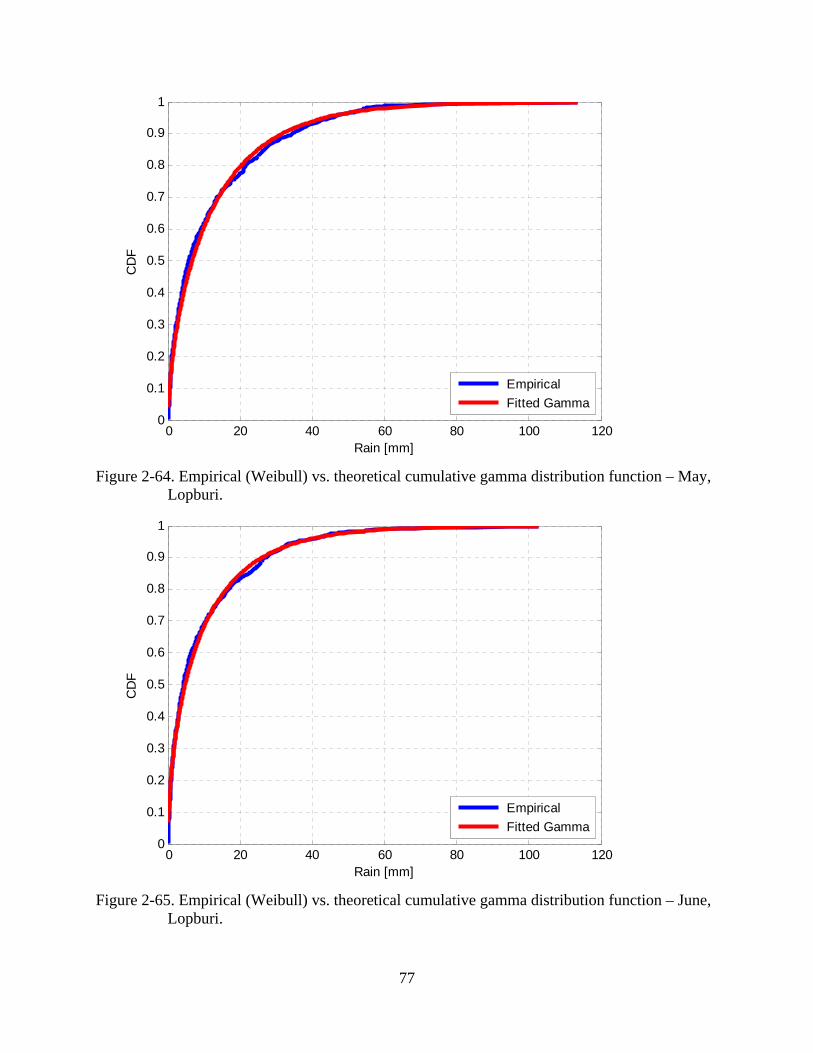
0 20 40 60 80 100 1200

0.1

0.2

0.3

0.4

0.5

0.6

0.7

0.8

0.9

1

Rain [mm]

CD

F


Figure 2-64. Empirical (Weibull) vs. theoretical cumulative gamma distribution function – May,

Lopburi.

0 20 40 60 80 100 1200

0.1

0.2

0.3

0.4

0.5

0.6

0.7

0.8

0.9

1

Rain [mm]

CD

F


Figure 2-65. Empirical (Weibull) vs. theoretical cumulative gamma distribution function – June,

Lopburi.

77

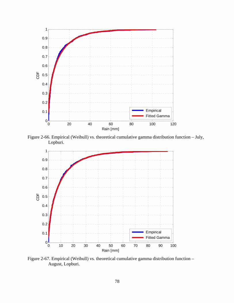
0 20 40 60 80 100 1200

0.1

0.2

0.3

0.4

0.5

0.6

0.7

0.8

0.9

1

Rain [mm]

CD

F


Figure 2-66. Empirical (Weibull) vs. theoretical cumulative gamma distribution function – July,

Lopburi.

0 10 20 30 40 50 60 70 80 90 1000

0.1

0.2

0.3

0.4

0.5

0.6

0.7

0.8

0.9

1

Rain [mm]

CD

F


Figure 2-67. Empirical (Weibull) vs. theoretical cumulative gamma distribution function –

August, Lopburi.

78

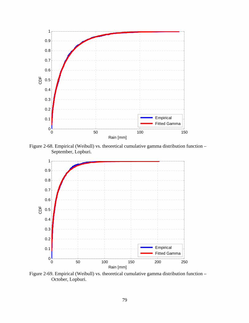
0 50 100 1500

0.1

0.2

0.3

0.4

0.5

0.6

0.7

0.8

0.9

1

Rain [mm]

CD

F



September, Lopburi.

0 50 100 150 200 2500

0.1

0.2

0.3

0.4

0.5

0.6

0.7

0.8

0.9

1

Rain [mm]

CD

F



October, Lopburi.

79

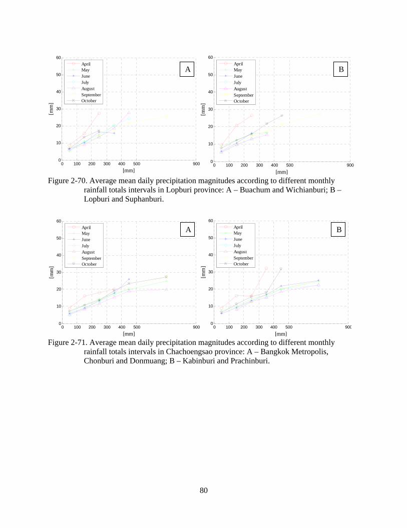
0 100 200 300 400 500 9000

10

20

30

40

50

60

[mm]

[mm

]

AprilMayJuneJulyAugustSeptemberOctober

0 100 200 300 400 500 9000

10

20

30

40

50

60

[mm]

[mm

]


A B

Figure 2-70. Average mean daily precipitation magnitudes according to different monthly rainfall totals intervals in Lopburi province: A – Buachum and Wichianburi; B – Lopburi and Suphanburi.

0 100 200 300 400 500 9000

10

20

30

40

50

60

[mm]

[mm

]


0 100 200 300 400 500 9000

10

20

30

40

50

60

[mm]

[mm

]


A B

Figure 2-71. Average mean daily precipitation magnitudes according to different monthly rainfall totals intervals in Chachoengsao province: A – Bangkok Metropolis, Chonburi and Donmuang; B – Kabinburi and Prachinburi.

80

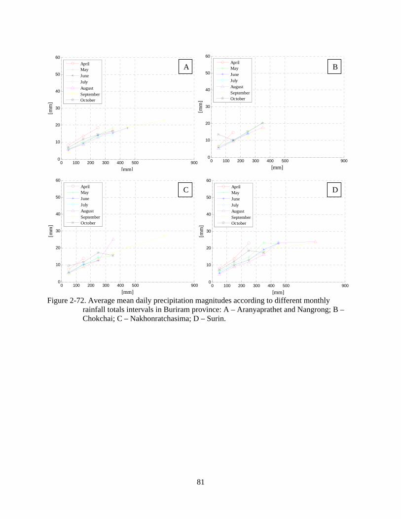
0 100 200 300 400 500 9000

10

20

30

40

50

60

[mm]

[mm

]


0 100 200 300 400 500 9000

10

20

30

40

50

60

[mm]

[mm

]


0 100 200 300 400 500 9000

10

20

30

40

50

60

[mm]

[mm

]


0 100 200 300 400 500 9000

10

20

30

40

50

60

[mm]

[mm

]


A B

C D

Figure 2-72. Average mean daily precipitation magnitudes according to different monthly rainfall totals intervals in Buriram province: A – Aranyaprathet and Nangrong; B – Chokchai; C – Nakhonratchasima; D – Surin.

81

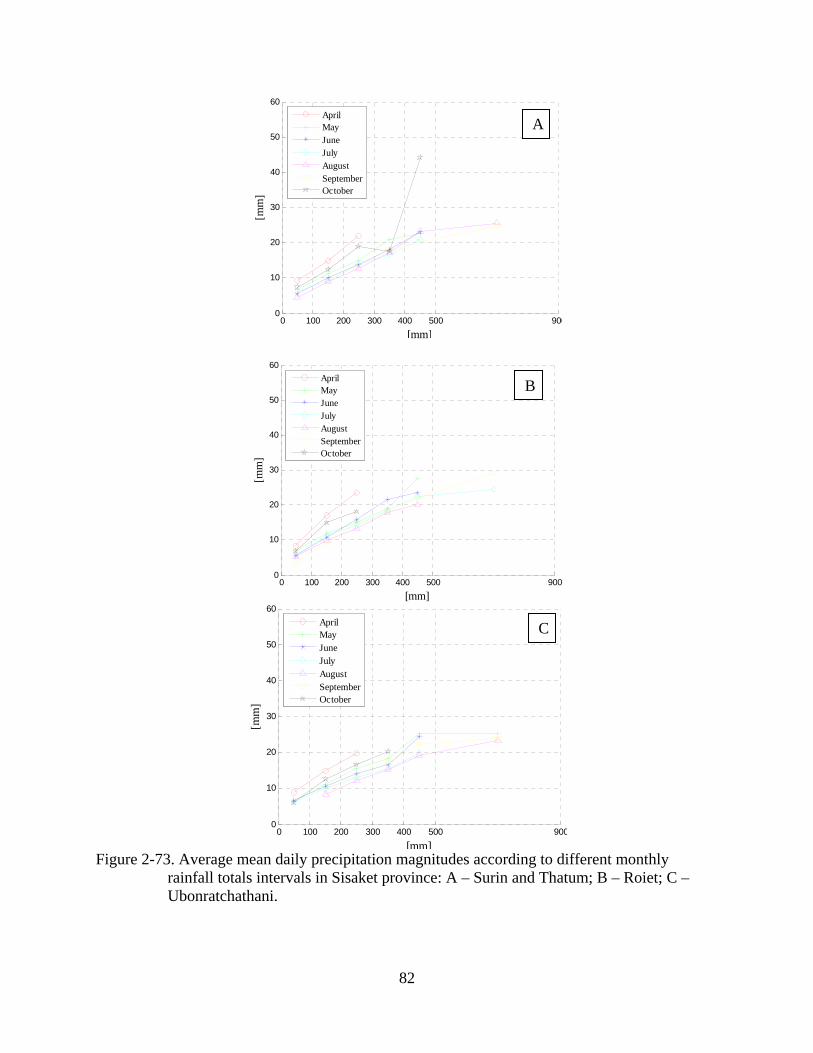
0 100 200 300 400 500 9000

10

20

30

40

50

60

[mm]

[mm

]


A

0 100 200 300 400 500 9000

10

20

30

40

50

60

[mm]

[mm

]


0 100 200 300 400 500 9000

10

20

30

40

50

60

[mm]

[mm

]


B

C

Figure 2-73. Average mean daily precipitation magnitudes according to different monthly rainfall totals intervals in Sisaket province: A – Surin and Thatum; B – Roiet; C – Ubonratchathani.

82

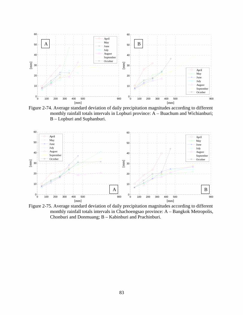
0 100 200 300 400 500 9000

10

20

30

40

50

60

[mm]

[mm

]


0 100 200 300 400 500 9000

10

20

30

40

50

60

[mm]

[mm

]


A B

Figure 2-74. Average standard deviation of daily precipitation magnitudes according to different monthly rainfall totals intervals in Lopburi province: A – Buachum and Wichianburi; B – Lopburi and Suphanburi.

0 100 200 300 400 500 9000

10

20

30

40

50

60

[mm]

[mm

]


0 100 200 300 400 500 9000

10

20

30

40

50

60

[mm]

[mm

]


A B

Figure 2-75. Average standard deviation of daily precipitation magnitudes according to different monthly rainfall totals intervals in Chachoengsao province: A – Bangkok Metropolis, Chonburi and Donmuang; B – Kabinburi and Prachinburi.

83

0 100 200 300 400 500 9000

10

20

30

40

50

60

[mm]

[mm

]


0 100 200 300 400 500 9000

10

20

30

40

50

60

[mm]

[mm

]


A B

0 100 200 300 400 500 9000

10

20

30

40

50

60

[mm]

[mm

]


0 100 200 300 400 500 9000

10

20

30

40

50

60

[mm]

[mm

]


C

D

Figure 2-76. Average standard deviation of daily precipitation magnitudes according to different monthly rainfall totals intervals in Buriram province: A – Aranyaprathet and Nangrong; B – Chokchai; C – Nakhonratchasima; D – Surin.

84

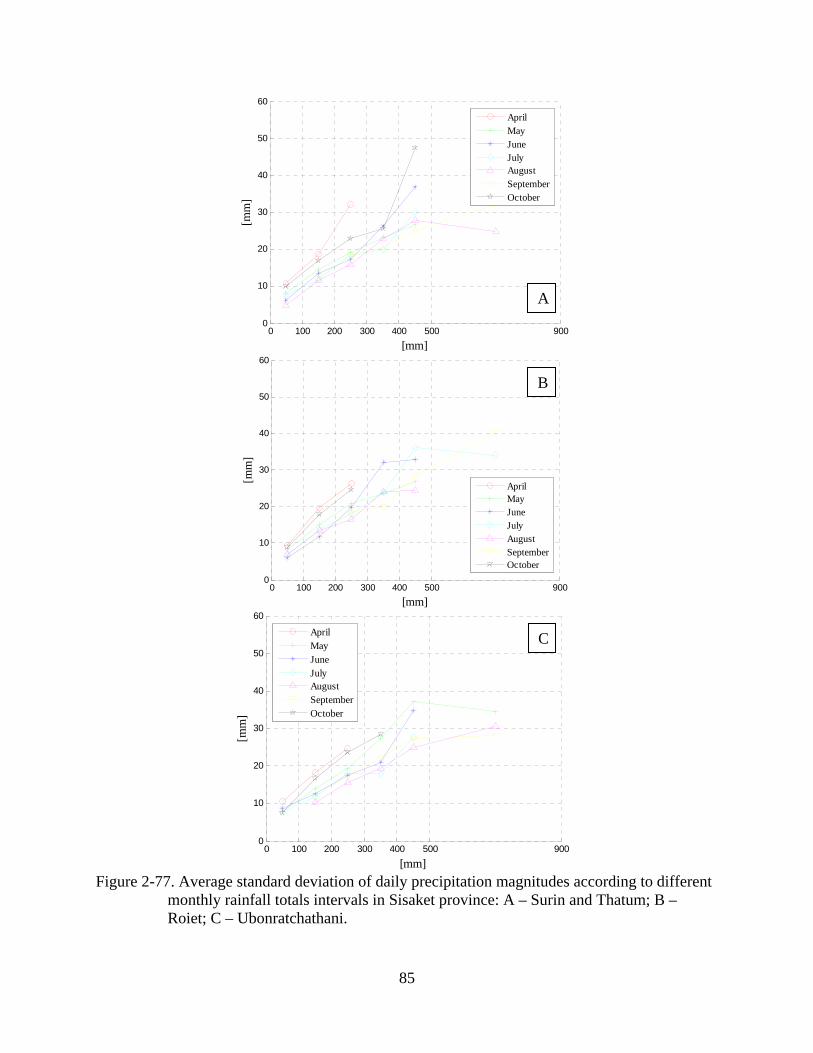
0 100 200 300 400 500 9000

10

20

30

40

50

60

[mm]

[mm

]


A

0 100 200 300 400 500 9000

10

20

30

40

50

60

[mm]

[mm

]


B

0 100 200 300 400 500 9000

10

20

30

40

50

60

[mm]

[mm

]


C

Figure 2-77. Average standard deviation of daily precipitation magnitudes according to different monthly rainfall totals intervals in Sisaket province: A – Surin and Thatum; B – Roiet; C – Ubonratchathani.

85

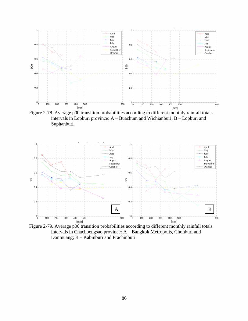
0 100 200 300 400 500 9000

0.2

0.4

0.6

0.8

1

[mm]

P00


0 100 200 300 400 500 9000

0.2

0.4

0.6

0.8

1y p [ ]

[mm]

P00


Figure 2-78. Average p00 transition probabilities according to different monthly rainfall totals

intervals in Lopburi province: A – Buachum and Wichianburi; B – Lopburi and Suphanburi.

0 100 200 300 400 500 9000

0.2

0.4

0.6

0.8

1y p [ ]

[mm]

P00


0 100 200 300 400 500 9000

0.2

0.4

0.6

0.8

1

[mm]

P00


A B

Figure 2-79. Average p00 transition probabilities according to different monthly rainfall totals intervals in Chachoengsao province: A – Bangkok Metropolis, Chonburi and Donmuang; B – Kabinburi and Prachinburi.

86

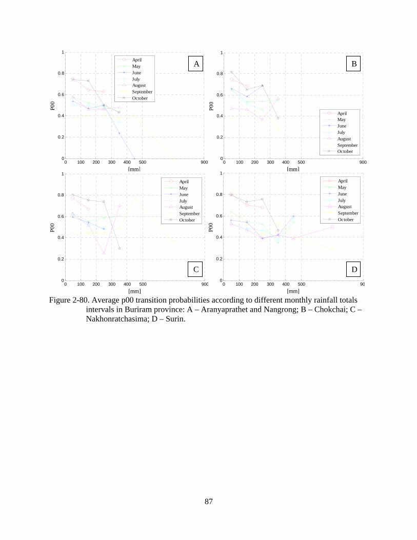
0 100 200 300 400 500 9000

0.2

0.4

0.6

0.8

1

[mm]

P00


0 100 200 300 400 500 9000

0.2

0.4

0.6

0.8

1

[mm]

P00


A B

0 100 200 300 400 500 9000

0.2

0.4

0.6

0.8

1

[mm]

P00


0 100 200 300 400 500 900

0.2

0.4

0.6

0.8

1

[mm]

P00


C D

Figure 2-80. Average p00 transition probabilities according to different monthly rainfall totals intervals in Buriram province: A – Aranyaprathet and Nangrong; B – Chokchai; C – Nakhonratchasima; D – Surin.

87

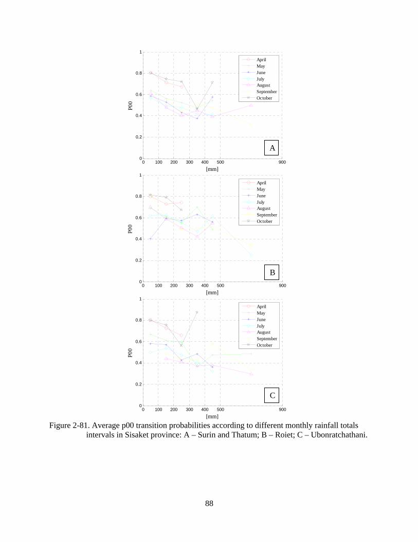
0 100 200 300 400 500 9000

0.2

0.4

0.6

0.8

1

[mm]

P00


A

0 100 200 300 400 500 9000

0.2

0.4

0.6

0.8

1

[mm]

P00


B

0 100 200 300 400 500 9000

0.2

0.4

0.6

0.8

1

[mm]

P00


C

Figure 2-81. Average p00 transition probabilities according to different monthly rainfall totals intervals in Sisaket province: A – Surin and Thatum; B – Roiet; C – Ubonratchathani.

88

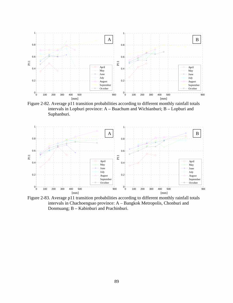
0 100 200 300 400 500 9000

0.2

0.4

0.6

0.8

1

[mm]

P11


0 100 200 300 400 500 9000

0.2

0.4

0.6

0.8

1

[mm]

P11


A B

Figure 2-82. Average p11 transition probabilities according to different monthly rainfall totals intervals in Lopburi province: A – Buachum and Wichianburi; B – Lopburi and Suphanburi.

0 100 200 300 400 500 9000

0.2

0.4

0.6

0.8

1

[mm]

P11


0 100 200 300 400 500 9000

0.2

0.4

0.6

0.8

1

[mm]

P11


A B

Figure 2-83. Average p11 transition probabilities according to different monthly rainfall totals intervals in Chachoengsao province: A – Bangkok Metropolis, Chonburi and Donmuang; B – Kabinburi and Prachinburi.

89

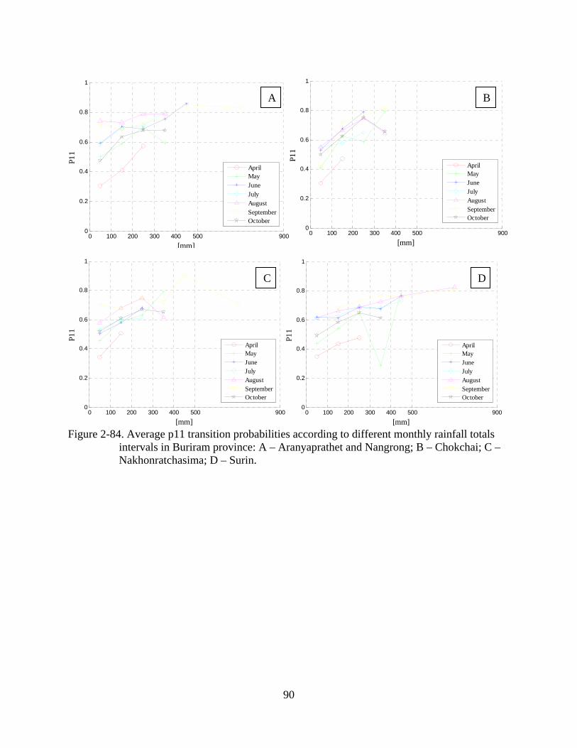
0 100 200 300 400 500 9000

0.2

0.4

0.6

0.8

1

[mm]

P11


0 100 200 300 400 500 9000

0.2

0.4

0.6

0.8

1

[mm]

P11


A B

0 100 200 300 400 500 9000

0.2

0.4

0.6

0.8

1

[mm]

P11


0 100 200 300 400 500 9000

0.2

0.4

0.6

0.8

1

[mm]

P11


C D

Figure 2-84. Average p11 transition probabilities according to different monthly rainfall totals intervals in Buriram province: A – Aranyaprathet and Nangrong; B – Chokchai; C – Nakhonratchasima; D – Surin.

90

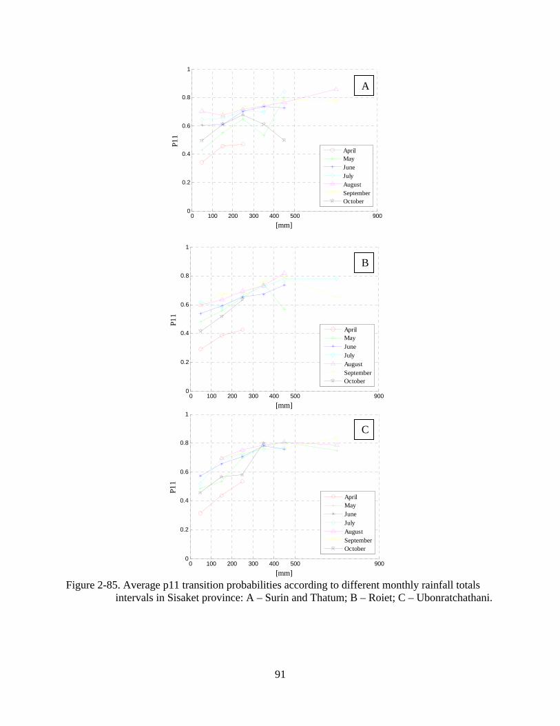
0 100 200 300 400 500 9000

0.2

0.4

0.6

0.8

1

[mm]

P11


A

0 100 200 300 400 500 9000

0.2

0.4

0.6

0.8

1

[mm]

P11


0 100 200 300 400 500 9000

0.2

0.4

0.6

0.8

1

[mm]

P11


B

C

Figure 2-85. Average p11 transition probabilities according to different monthly rainfall totals intervals in Sisaket province: A – Surin and Thatum; B – Roiet; C – Ubonratchathani.

91

CHAPTER 3 CONCLUSIONS

In many areas of Thailand, climate shocks have profound effects on livelihoods and the

economy on a local and national scale. As in most countries whose revenue structure is highly

dependent on agriculture, the consequences of climatic extremes can have damaging effect on

the crop yields and therefore on both national and household incomes (Boochabun et al. 2004).

This effect is even more profound in less developed regions with monocultural agriculture and

less developed irrigation systems (Kono and Saha 1995; Yao 1997). This study focused on two

regions of Thailand – central and northeast with the center being relatively wealthy, diversified

and irrigated, and the latter relatively poor, less diversified and in large percent consisting of

rain-fed arable land.

Consequently, the ability to assess the probability of excess or dearth of rainfall

occurrences is an essential aspect for planning both for the national economy and insurance

companies investing the Thai region. For the decision making process it is crucial that farmers

have an appealing and straightforward way to assess the risk of unfavorable agro-meteorological

conditions that occur in their region. This method showed to be flexible enough that it could be

applied for a variety of crops. At the same time, the insurance companies are interested in

knowing the risk of potential agro-climatic shock occurrences in order to set premiums that

would not bring losses to their enterprises.

This study looks at a series of daily rainfall properties that could potentially constitute the

climatic shock at the socio-economic survey locations. These surveys provide an important link

between environmental variables and information about local farmers and their income. It was

important to assess how past weather conditions can be determined from monthly rainfall totals,

so that this information can be linked to the financial well-being of the local people. Neighboring

92

national network stations provide invaluable insight into longer climate variability and

fluctuations, and allow assessment of the probability of the climate shocks that occurred in the

past and could occur in the future. Located within a close distance to the survey locations, the

data collected at these stations can represent with high likelihood conditions that occurred in

locations where no daily data is available. The chosen rainfall parameters are crucial in

determining extreme conditions like flood or drought. These parameters include the transition

probability of a day with no rain to be followed by a day with no rain and for the rainy day to be

followed by a consecutive rainy day. The second important characteristics are the rainfall

magnitudes and the likelihood of extremely low or high daily rainfall totals. One unique example

of this site is that the daily rainfall precipitation has been shown to follow gamma distribution

properties and is highly sensitive to changes in the rainfall transition probabilities throughout the

season and at various locations. This result can be attributed to the convective precipitation

pattern in the season and highly variable number and sequence of daily rainfall.

The outcome of this study provides insight into statistical examination of precipitation

properties which is less studied in tropical areas compared to temperate regions, where long time

daily rainfall records are more abundant. On the macro-regional scale, there is considerably less

research done in the area of Southeast Asia compared to South Asia with the focus on India and

East Asia with the focus on China (Stephenson et al. 1999; Krishnamurthy and Goswami 2000;

Ding and Chan 2005; Ding 2007; Yancheva et al. 2007). This refers both to the research

regarding the monsoon properties and likewise the ENSO impact on the interannual variability of

rainfall. This is however an equally important issue in the entire region of South, Southeast and

East Asia, where agriculture is one of the essential parts of the economy and household incomes.

93

While this research is focused exclusively on the rainfall characteristics of four provinces

in Thailand, the results provide important means of understanding similar problems on the larger

national scale and possibly in many other areas of the globe, especially in the monsoonal areas of

the Southeast Asia and possibly in other tropical countries. This method can be applied for any

problems looking at the probability of extreme events to happen not only in climatology, but also

in a many sections of geography and possibly in many other scientific disciplines.

94

LIST OF REFERENCES

Barger, G. L., and H.C.S. Thom, 1949: Evaluation of drought hazard. Agronomy Journal, 41, 519–526.

Boochabun, K., W. Tych, N. A. Chappell, P. A. Carling, K. Lorsirirat, and S. Pa-Obsaeng, 2004: Statistical modeling of rainfall and river flow in Thailand. Journal Geological Society of India, 64, 503-516.

Caskey, J. E., 1963: A Markov chain model for the probability of precipitation occurrence in intervals of various length. Monthly Weather Review, 91, 298-301.

Coe, R., and R.D.Stern, 1982: Fitting models to daily rainfall data. Journal of Applied Meteorology, 21, 1024-1031.

Cunnane, C., 1978: Unbiased plotting positions - A review. Journal of Hydrology, 37, 205-222.

Ding, Y., 2007: The variability of the Asian summer monsoon. Journal of the Meteorological Society of Japan, 85B, 21-54.

Ding, Y., and J. C. L. Chan, 2005: The East Asian summer monsoon: an overview. Meteorology and Atmospheric Physics, 89, 117-142.

Gadgil, S., and K. R Kumar, 2006: The Asian monsoon – agriculture and economy. The Asian Monsoon, B. Wang, Ed., Springer, 844 pp.

Gates, P., and H. Tong, 1976: On Markov chain modeling to some weather data. Journal of Applied Meteorology, 15, 1145-1151.

Gleick, P. H. 1993: Water in Crisis: A Guide to the World’s Fresh Water Resources. Oxford University Press, 473 pp.

Guzman, A. G., and W. C. Torrez, 1985: Daily rainfall probabilities: Conditional upon prior occurrence and amount of rain. Journal of Climate and Applied Meteorology, 24, 1009-1014.

Harrison, M., and P. R. Waylen, 2000: A note concerning the proper choice for Markov model order for daily precipitation in the humid tropics: A Case Study in Costa Rica. International Journal of Climatology, 20, 1861-1872.

Hosking, J. R. M., and J. R. Wallis, 1987: Parameter and quantile estimation for the generalized Pareto distribution. Technometrics, 29, 339-349.

Huang, Y., C. Lee, and C. Ting, 2008: Improved estimation of hydrologic data using the Chi-square goodness-of-fit test. Journal of the Chinese Institute of Engineers, 31, 515-521.

Ison, N.T., A.M. Feyerherm, and L.D. Bark, 1971: Wet period precipitation and the gamma distribution. Journal of Applied Meteorology, 10, 658–665.

95

Katz, R. W., 1977: Precipitation as chain-dependent process. Journal of Applied Meteorology, 16, 671-676.

Katz, R. W., 1981: On some criteria for estimating the order of a Markov chain. Technometrics, 23, 243-249.

Kermel-Torrès, D., 2004: Atlas of Thailand: Spatial Structures and Development. Silkworm Books, 209 pp.

Khedari, J., A. Sanprajak, and J. Hirunlabh, 2002: Thailand climatic zones. Renewable Energy, 25, 267-280.

Kono, Y., and P.K. Saha, 1995: Land and water resources management for crop diversification in the Chao Phraya Delta, Thailand: A case study of citrus cultivation in the North Rangsit Irrigation Project. Southeast Asian Studies, 33, 169-186.

Kripalani, R. H., and A. Kulkarni, 1997: Rainfall variability over South-East Asia – Connections with Indian monsoon and ENSO extremes: New perspectives. International Journal of Climatology, 17, 1155-1168.

Krishna Kumar, K., B. Rajagopalan, and M. A. Cane, 1999: On the weakening relationship between the Indian monsoon and ENSO. Science, 284, 2156-2159.

Krishnamurthy, V., and B. N. Goswami, 2000: Indian monsoon – ENSO relationship on interdecadal timescale. Journal of Climate, 13, 579–595.

Lau, K. M., and S. Yang, 1997: Climatology and interannual variability of the Southeast Asian summer monsoon. Advances in Atmospheric Sciences, 14, 141-16.

Lü, J., Q. Zhang, S. Tao, and J. Ju, 2006: The onset and advance of the Asian summer monsoon. Chinese Science Bulletin, 51, 80-88.

Madsen, H., P. F. Rasmussen, and D. Rosbjerg, 1997: Comparison of annual maximum series and partial duration series methods for modeling extreme hydrologic events. 1. At-site modeling. Water Resources Research, 33, 747-757.

Mendelsohn, R., 2007: What causes crop failure?. Climatic Change, 81, 61-70.

Mendelsohn, R., A. Basist, A. Dinar, P. Kurukulasuriya, and C. Williams, 2007: What explains agricultural performance: climate normals or climate variance?. Climatic Change, 81, 85-99.

Murdiyarso, D., 2000: Adaptation to climatic variability and change: Asian perspectives on agriculture and food security. Environmental Monitoring and Assessment, 61, 123-131.

Paxson, C. H., 1992: Using weather variability to estimate the response of savings to transitory income in Thailand. The American Economic Review, March, 15-32.

96

Rosbjerg, D., H. Madsen, and P. F. Rasmussen, 1992: Prediction in partial duration series with generalized Pareto-distributed exceedances. Water Resources Research, 28, 3001-3010.

Shenton, L. R., and K. O. Bowman, 1973: Note on the sample size to achieve normality for estimators for the gamma distribution. Monthly Weather Review, 101, 891–892.

Singhrattna, N., B. Rajagopalan, K. Krishna Kumar, and M. Clark, 2005: Interannual and interdecadal variability of Thailand summer monsoon season. Journal of Climate, 18, 1697-1708.

Stephenson, D. B., K. Rupa Kumar, F. J. Doblas-Reyes, J. F. Royer, and F. Chauvin, 1999: Extreme daily rainfall events and their impact on ensemble forecasts of the Indian monsoon. Monthly Weather Review, 127, 1954-1966.

Stern, R.D. and R. Coe, 1984: A model fitting analysis of daily rainfall data. Journal of Royal Statistical Society, 147, 1-34.

Thom, H.C.S., 1958: A note on the gamma distribution. Monthly Weather Review, 86, 117–122.

Wackerly, D. D., W. Mendenhall III, and R. L. Scheaffer, 2002: Mathematical Statistics with Applications. Duxbury, 853 pp.

Wilks, D. S., 1998: Multisite generalization of a daily stochastic precipitation generation model. Journal of Hydrology, 210, 178-191.

Wilks, D. S., and R. L. Wilby, 1999: The weather generation game: a review of stochastic weather models. Progress in Physical Geography, 23, 329-357.

Wilks, D. S., 2006: Statistical Methods in the Atmospheric Sciences. Academic Press, 627 pp.

Yancheva, G., N. R. Nowaczyk, J. Mingram, P. Dulski, G. Schettler, J. F. W. Negendank, J. Liu, D. M. Sigman, L. C. Peterson, and G. Haug, 2007: Influence of the intertropical convergence zone on the East Asian monsoon. Nature, 445, 74-77.

Yao, S., 1997: Comparative advantages and crop diversification: A policy analysis matrix for Thai agriculture. Journal of Agricultural Economics, 48, 211-222.

97

98

BIOGRAPHICAL SKETCH

Anna Szyniszewska was born in Poznan, Poland. She received Bachelor of Arts degree in

Tourism and Leisure from the Adam Mickiewicz University, Department of Geographical and

Geological Sciences in Poznan, Poland in 2003. She spent 1.5 years in Japan where she attended

the Kanazawa University as a part-time student and research assistant on the Hovsgol Drilling

Project - research on long-term climate changes in Central Asia.

Her interest in climatology brought her to the University of Florida to pursue her master’s

degree. She plans to continue her education at the University of Florida to the doctorate level.

© 2009 Anna Maria Szyniszewska

Documents

Transcript of © 2009 Anna Maria Szyniszewska