Copyright 2002 David M. Hassenzahl Using r and 2 Statistics for Risk Analysis.

2002
David M. Hassenzahl
Exploring Carcinogen Risk Analysis Through Benzene
Image from Matthew J. DowdDepartment of Medicinal ChemistryVirginia Commonwealth University

2002
David M. Hassenzahl
Objective
• Use benzene as a case for exploring
• Toxicology
• Epidemiology
• Uncertainty
• Regulatory Science

2002
David M. Hassenzahl
Toolbox Building
• Likelihood Maximization
• Curve fitting
• Bootstrapping
• Z-Scores
• Relative Risk
• Dose-Response extrapolation

2002
David M. Hassenzahl
Overview of benzene
• Fairly common hydrocarbon– Manufacturing– Petroleum products
• Strongly suspected human carcinogen– Animal assays– Many epidemiological studies– Leukemia as important endpoint

2002
David M. Hassenzahl
Benzene structure
Image from Matthew J. DowdDepartment of Medicinal ChemistryVirginia Commonwealth University

2002
David M. Hassenzahl
Benzene Data in Should We Risk It?
• Toxicological Data, p. 175 et seq.
• Epidemiological Data p 211 – 216
• But many other data sets– Other toxicological data (rare)– Chinese workers– Turkish workers

2002
David M. Hassenzahl
Toxicology Data Set
Number of mice
Mice with tumors
Mouse dose
50 0 0
50 4 14
50 20 27
50 37 59
Crump and Allen 1984

2002
David M. Hassenzahl
What are risks from benzene?
• Risk as potency times exposure
• How do we determine potency?– Extrapolate from animal data?– Extrapolate from epidemiological data?– How wrong will we be?
• What are “real” exposures?– What are effects at these levels?

2002
David M. Hassenzahl
Toxicology
• Paracelsus “the dose makes the poison”
• Regulatory assumptions!
• This is not Dr. Gerstenberger’s Toxicology!

2002
David M. Hassenzahl
Reading
• SWRI Chapter 5
• US EPA Proposed guidelines (US EPA 1996)
• Cox 1996

2002
David M. Hassenzahl
General idea
• Applied doses– Greater specificity about exposure than
epidemiology
• Observed effects
• Artificial control of exposure

2002
David M. Hassenzahl
Physiologically Based Pharmacokinetics
• PBPK
• Investigate flows of materials through bodies
• System dynamics models
• More on these in exposure lecture

2002
David M. Hassenzahl
Studies
• Animals– Rarely humans
• Parts– Cell– tissue

2002
David M. Hassenzahl
Effects
• Chronic – cancer fatality– increasing interest in other issues– lead and intelligence in children.
• Acute– Reversible – Irreversible

2002
David M. Hassenzahl
Crump and Allen Benzene data set
• Animals at various concentrations
• Four data points
• “Designer” mice

2002
David M. Hassenzahl
Relevance to Humans
• How to get from
• high level, lifetime studies of animals
to
• anticipated low dose effects in humans?

2002
David M. Hassenzahl
Questions about benzene
• Is benzene a mouse carcinogen?
• Is benzene a human carcinogen?
• If so, how potent?

2002
David M. Hassenzahl
Crump and Allen data set (Crump and Allen 1984)Note: the actual doses are not stated correctly here. See “notes for more information
Benzene data set INumber of Test mice
Number of Mice with tumors
Mouse Test Dose (mg/kg/d) (Oral gavage)
50 0 0 50 4 25 50 20 50 50 37 100

2002
David M. Hassenzahl
Crump and Allen data set.
Benzene data set II
P(c
ance
r)
0
0.2
0.4
Dose (mg/kg/day)
0 25 50 75 100
1.0
0.8
0.6

2002
David M. Hassenzahl
Uncertainty Pervades
• Often understated
• Creates (or at least prolongs) conflict
• Think as we go! (Part of Homework PS 2)

2002
David M. Hassenzahl
Animal Test Issues
• Interspecific comparison
• Statistical uncertainty
• Heterogeneity
• Extrapolation
• Dose Metric

2002
David M. Hassenzahl
Interspecific comparison
• Mouse-human– Metabolism as a function of body weight
– Dosehuman = sf Dosemouse
– sf = (BWhuman/BWmouse)1-b
– b is empirically derived as 0.75a
a. See SWRI page 177.

2002
David M. Hassenzahl
Interspecific comparison
• Lifetime of human = lifetime mouse?– Mice age 30 days per human day– Total mouse lifetime is much shorter
• Analogous organs or processes?– Do mice have cancer points we do not?– Do we have cancer points mice do not?
a. See SWRI page 177.

2002
David M. Hassenzahl
Species Sex Std. Adult BW (kg1,2)
Human Male 78.7 Female 65.4 Both 71.0 Rat Male 0.5 Female 0.35 Mouse Male 0.03 Female 0.025
1. Hallenbeck, 19932. Finley et al.,
1994
Interspecific comparison

2002
David M. Hassenzahl
sf = (BWhuman/BWmouse)1-b
sf = (70/0.03)0.25 = 7.0Dosehuman = 7.0 Dosemouse
Number of Test mice
Number of Mice with tumors
Mouse Test Dose (mg/kg/day) (Oral gavage)
Equivalent human dose (mg/kg/day)
50 0 0 50 4 25 50 20 50 50 37 100
Interspecific comparison

2002
David M. Hassenzahl
Crump and Allen data set, converted to humans
Number of Test mice
Number of Mice with tumors
Mouse Test Dose (mg/kg/day) (Oral gavage)
Equivalent human dose (mg/kg/day)
50 0 0 0 50 4 25 175 50 20 50 350 50 37 100 700
Interspecific comparison

2002
David M. Hassenzahl
Animal Test Issues
• Interspecies comparison
• Statistical uncertainty
• Heterogeneity
• Extrapolation
• Dose Metric

2002
David M. Hassenzahl
Binomial Distribution
• 50 genetically “identical” mice…binomial distribution?
• Can use this to generate “likelihood function” to compare the likelihood that any given probability is

2002
David M. Hassenzahl
Likelihood Maximization
• More appropriate than Least Squares when you know something about likelihoods
• “Bootstrapping” method needed
• We will work through likelihood maximization

2002
David M. Hassenzahl
Can calculate standard deviation using the binomial
npps 1
Recall that two standard deviations to either side represents a 95% confidence interval, and...
Statistical Uncertainty

2002
David M. Hassenzahl
Crump and Allen data set, applied to humans
P(c
ance
r)
0
0.2
0.4
Human Dose (mg/kg/day)
0 175 350 525 700
1.0
0.8
0.6
Statistical Uncertainty

2002
David M. Hassenzahl
Animal Test Issues
• Interspecies comparison
• Statistical uncertainty
• Heterogeneity
• Extrapolation
• Dose Metric

2002
David M. Hassenzahl
Heterogeneity
• Epidemiology and toxicology
• Genetically identical mice compared to diverse humans
• Predictable versus unpredictable susceptibility
• Male and female differences (observed cancer rates are different)

2002
David M. Hassenzahl
Heterogeneity
• Genetic diversity among humans
• Early insights into cancer mechanism: subpopulation born with one of two “steps” competed
• Variability as a function of age

2002
David M. Hassenzahl
Animal Test Issues
• Interspecies comparison
• Statistical uncertainty
• Heterogeneity
• Extrapolation
• Dose Metric

2002
David M. Hassenzahl
Extrapolation
• Theoretical or “Mechanistic” models: – one-hit – two-hit– two-stage
• Empirical – Cox “data-driven, model free curve fitting”
• EPA Proposed Guidelines

2002
David M. Hassenzahl
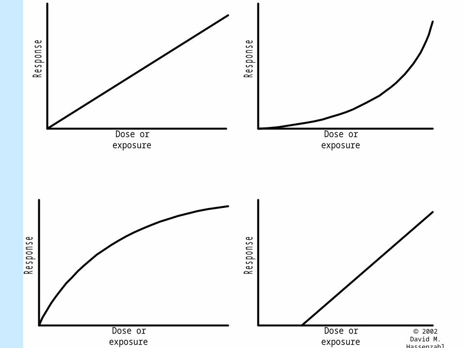
Extrapolation Concerns
Overestimation• Tautological
effects• Thresholds• Hormesis, or
“Vitamin” effect
Underestimation• Saturation• Synergistic effects• Susceptibility• Omission
2002
David M. Hassenzahl
Res
pons
e
Dose orexposure
Res
pons
e
Dose orexposure
Res
pons
e
Dose orexposure
Res
pons
e
Dose orexposure

2002
David M. Hassenzahl
Extrapolation Range Observed RangeR
espo
nse
10%
0%
HumanExposureof Interest
LED 10 ED 10
Dose
Projected Linear
(Con
fiden
ce Li
mit on D
ose)
(Cen
tral E
stim
ate)
After EPA (1996)

2002
David M. Hassenzahl
Crump and Allen data set, applied to humans
P(c
ance
r)
0
0.2
0.4
Human Dose (mg/kg/day)
0 175 350 525 700
1.0
0.8
0.6
Statistical Uncertainty

2002
David M. Hassenzahl
P(ca
ncer
)
0
0.2
0.4
Human Dose (mg/kg/day)
0 175 350 525 700
1.0
0.8
0.6
LED(10) =100 mgb/kg/day

2002
David M. Hassenzahl
If LED(10) = 100 mg/kg/day, then
LED(10-6) = 100 10-6 / 0.1 = 1 10-4 mg/kg/day
Extrapolation

2002
David M. Hassenzahl
Animal Test Issues
• Interspecies comparison
• Statistical uncertainty
• Heterogeneity
• Extrapolation
• Dose Metric

2002
David M. Hassenzahl
Dose Metric
• Assumption: exposure is irrelevant to effect
• Area under the curve/expected value.
• Lifetime dose leads to average daily dose.
• Particularly problematic if there are threshold effects or extreme effects

2002
David M. Hassenzahl
Risk to Humans?
• Lifetime cancer risk
• 40 hours per week
• 50 weeks per year
• 30 years
• Average 10 ppm(v) exposure?

2002
David M. Hassenzahl
Calculate Risk
• 10ml benzene/liter air
• 0.313 ml/mg
• 20m3 air / day
• 1000 liters/ m3
• 70kg person

2002
David M. Hassenzahl
• Lifetime Cancer Probability is a function of Dose and Potency
• Assume cumulative dose– Use Daily Dose per kg body weight,
averaged over lifetime
• Potency usually given as q*– Additional risk per unit dose
Cancer Risk
lifetime*b ADDqLCP(D)

2002
David M. Hassenzahl
exposedexposurelifetime fADDADD
LHpWWpYYpLf exposed
factors conversionBWIRCADD -1airb,exposure
Cancer Risk: Exposure Term

2002
David M. Hassenzahl
Computed Exposure Terms
b
b
b
b3air
3air
bexposure mmole
78mg
ml
e0.0446mmol
70kg
1
day
20m
m
10mlADD
daykg
69.6mgADD b
exposure
8760HpY70YpL
40HpW50WpY30YpLf exposed
098.0f exposed

2002
David M. Hassenzahl
Computed Exposure Terms
daykg
69.6mgADD b
exposure
098.0f exposed
exposedexposurelifetime fADDADD
daykg
6.8mg098.0
daykg
69.6mgbADD b
lifetime

2002
David M. Hassenzahl
Cancer Risk
lifetime*b ADDqLCP(D)
daykg
mg8.6ADD b
lifetime
001.0100mg
daykg1.0q
b
*b
007.0daykg
6.8mg
mg
daykg001.0LCP(D) b
b

2002
David M. Hassenzahl
“Regulatory Science” Issues
• Neither a simple question nor a mindless approach– (although often stated this way)
• “Human health conservative” versus• “Heavy hand of conservative
assumptions?”– May be overestimates– May be underestimates

2002
David M. Hassenzahl
Regulatory Toxicology
• “Real risk” is a reified risk
• ALL estimates, including central tendencies, are probably wrong
• More science does not guarantee – “less risk” – “less uncertainty”

2002
David M. Hassenzahl
Likelihood Maximization
A curve fitting technique

2002
David M. Hassenzahl
Binomial Distribution
• 50 genetically “identical” mice…binomial distribution?
• Can use this to generate “likelihood function” for a predicted outcome given an observed outcome

2002
David M. Hassenzahl
Likelihood Maximization
• More appropriate than Least Squares when you know something about likelihoods
• “Bootstrapping” method needed

2002
David M. Hassenzahl
Can calculate standard deviation using the binomial
npps 1
Recall that two standard deviations to either side represents a 95% confidence interval, and...
Statistical Uncertainty

2002
David M. Hassenzahl
Crump and Allen data set, applied to humans
P(c
ance
r)
0
0.2
0.4
Human Dose (mg/kg/day)
0 100 200 300 400
1.0
0.8
0.6
Statistical Uncertainty

2002
David M. Hassenzahl
Counting Rules
• What is the likelihood of getting 13 heads on 50 flips of a fair coin?
• We know the EXPECTED value– Expected value is 25 heads
XNXqp
!XNX!
N!P(X)

2002
David M. Hassenzahl
Binomial Developed
P(13|50) =
0.000315
P(25|50) = 0.112
P(37|50) = 0.000315
P(24|50) = 0.108
P(50|50) = 8.88 E-16
P(20|50) = 0.0412
Can use function in excel
1350130.50.5
!135013!
50!P(13)

2002
David M. Hassenzahl
Binomial, n = 50, p = 0.5
0
0.02
0.04
0.06
0.08
0.1
0.12
0 10 20 30 40 50 60

2002
David M. Hassenzahl
Likelihood
• Given– We’ve tested 50 mice at a dose Di
– We found a cancer rate P(Di)
• We expect that if we do it again, we will get the same rate
• We acknowledge that there’s some randomness

2002
David M. Hassenzahl
Fitting a model
• We know that our model can’t fit ALL the data points exactly
• P(100mg/kg/day) = 0.08, etc
• Let’s get as close to this as we can!
• Let’s “maximize the likelihood”

2002
David M. Hassenzahl
Likelihood Function
• From the binomial, we can derive the likelihood function
• Likelihood {P*(Di)|P(Di) is
• We don’t care the exact likelihood…we just want it as big as possible
iiDP1n
i*nDP
i* DP1DP
2002
David M. Hassenzahl
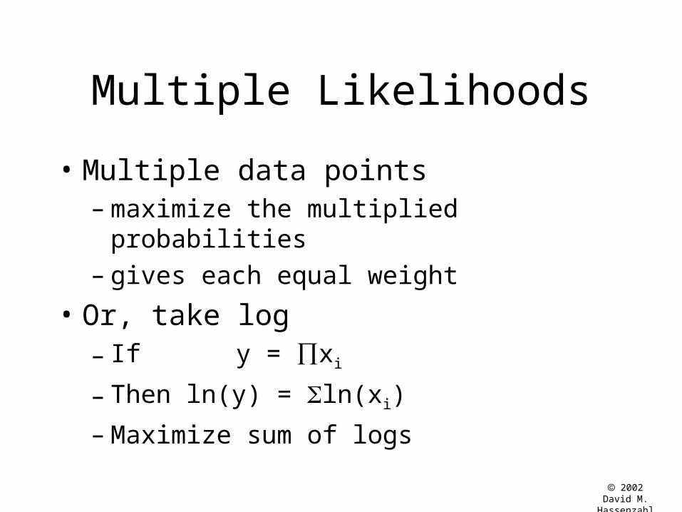
Multiple Likelihoods
• Multiple data points– maximize the multiplied probabilities – gives each equal weight
• Or, take log– If y = xi
– Then ln(y) = ln(xi)
– Maximize sum of logs

2002
David M. Hassenzahl
Simple Model
• P*(D) = kD + D0
• Hypothetical data set
n Dose P(Cancer|Dose)
50 0 0.02
50 500 0.04
50 1000 0.10
50 2000 0.18

2002
David M. Hassenzahl
Bootstrap
• Simple method to fit a model to data
• Akin to the game “hotter-colder”
• Optimizes a function– Least squares– Maximum likelihood
• Varies model parameters – hotter or colder

2002
David M. Hassenzahl
Bootstrap for benzene data set
• Create equation where
• Give known– P(Di), Di
• P*(D) = k*D + P*0
• Allow bootstrap to vary k*, P*0
• Maximize sum of log-likelihoods

2002
David M. Hassenzahl
Epidemiology for Risk Analysis
An Introduction

2002
David M. Hassenzahl
Objective
• Explore types of epidemiology methods• Understand the value and limitations of
epidemiology– Bradford-Hill criteria
• Learn essential epidemiology calculations
• Address benzene risk using epidemiological data

2002
David M. Hassenzahl
Overview of epidemiology
• Exposed human populations
• Hard to control
• Rarely addresses causality
• Common measures– Relative Risk – Z-scores

2002
David M. Hassenzahl
Pliofilm Cohort Data(SWRI Page 215)
Cumulative Exposure
ppm-years
Leukemia
Range Mean Person years
Observe deaths
Expected per pers-yr
0-45 11 30482 6 2.02E-4
45-400 151 16320 6 2.35E-4
400-1000 602 4667 3 3.39E-4
>1000 1341 915 6 4.81E-4
Total 132 52584 21 2.30E-4

2002
David M. Hassenzahl
Two Major Classes
Descriptive• Population Studies• Case Reports• Case Series• Cross-Sectional
Analyses
Analytical• Intervention Studies• Cohort Studies• Case-Control
studies Toxicology?

2002
David M. Hassenzahl
Uncertainty Issues
• Many toxicology uncertainties apply!
• Statistical uncertainty
• Heterogeneity
• Extrapolation
• Dose Metric

2002
David M. Hassenzahl
Population
• Also called “Correlational”
• Most of what we call “environmental epidemiology
• Not controlled
• No causation
• Can point us in the right direction
Note: this and subsequent slides draw heavily on Gots (1993)

2002
David M. Hassenzahl
Populations: pros and cons
• Large samples
• Can address – major effects – potential causes
• Low relative risk ratios
• Study design challenges

2002
David M. Hassenzahl
Case studies
• Observed correlation
• Event and outcome
• Examples – mobile phones and brain tumors– “Cancer clusters”
• No control group!
• A starting point only
2002
David M. Hassenzahl
Cross-sectional analysis
• One time deal
• Bunch of questions or data points

2002
David M. Hassenzahl
Intervention studies
• Common in medicine
• Double-blind
• Placebo
• Treatment
• Some ethical issues

2002
David M. Hassenzahl
Case-control
• Retrospective method
• One group with effect
• Comparable group without effect
• Observed differences in possible causes

2002
David M. Hassenzahl
Cohort studies
• Retrospective or prospective
• Look at exposure groups
• Compare rates of effects

2002
David M. Hassenzahl
Case-control
Pros• Rare / long latency
outcomes• Efficient / small
samples• Existing data• Range of causes /
exposures
Cons• Reconstructed
exposure• Data hard to
validate• Confounders• Selection of control• Can’t calculate rates• Causation unknown

2002
David M. Hassenzahl
Cohort Studies
Pros• Compares Exposures• Multiple outcomes• Complete data
– Cases– Stages
• Some data quality control
Cons• Large samples• Long-term commitment
– Funding and researchers– Subjects
• Extraneous factors• Expensive• Causation rare

2002
David M. Hassenzahl
Bradford-Hill Criteria (determining causation)
• Temporality (Chronological relationship)
• Strength of Association
• Intensity or duration of exposure
• Specificity of Association
• Consistency
• Coherence and biological plausibility
• Reversibility

2002
David M. Hassenzahl
Temporality
• Chronological relationship
• Does the presumed cause precede the effect?
• A cause must precede its effect
• This does not imply the reciprocal

2002
David M. Hassenzahl
Strength of Association
• High relative risk of acquiring the disease
• Strong p-value (low statistical uncertainty)

2002
David M. Hassenzahl
Intensity
• Also duration of exposure
• As exposure increases
• Does proposed effect increase?
2002
David M. Hassenzahl
Specificity of Association.
• Highly specific case
• Highly specific exposure
• Example: – “leukemia from benzene”
versus– “cancer from hydrocarbons”

2002
David M. Hassenzahl
Consistency
• If multiple findings
• Do all point the same way?
• “Meta-analysis” is common (SWRI page 373 - 377

2002
David M. Hassenzahl
Coherence and biological plausibility
• Postulate a mechanism
• Consistent with our understanding of biological processes
• Better if supporting toxicological data

2002
David M. Hassenzahl
Reversibility
• Does removal of a presumed cause lead to a reduction in the risk of ill-health?– MAY strengthen cause-effect relationship
• May suffer from similar fallacies as temporality

2002
David M. Hassenzahl
Some Correlation Issues
• Uncertain dosimetry– very difficult to estimate exposure
• Latency of effects, especially cancer
• Confounding factors
• Bias
• Representativeness of control group
• Small numbers
2002
David M. Hassenzahl
Risk in the Time of Cholera
• Famous case
• SWRI 207 to 211
• See Gots (1993) and Aldrich and Griffith (1993)
• …and almost any other epidemiology or statistics text!
2002
David M. Hassenzahl
Cholera in London, mid1800’s
• John Snow
• Drinking water from the Thames
• High rates of cholera
• Unknown cause of cholera– Ill humours?– Vapours?

2002
David M. Hassenzahl
Cholera in London mid 1800’s
• Many water companies– Southwark and Vauxhall, downstream– Lambeth, upstream– Several others

2002
David M. Hassenzahl
London Cholera Data 1853-4
Water Company
Number of Houses
Cholera Deaths
Southwark and Vauxhall
40,046 1,263
Lambeth 26,107 98
Rest of London
256,423 1,422

2002
David M. Hassenzahl
Assumptions
• No confounders, selection problems– Snow did a good job of this, we think
• Number of people per household– SWRI used 1 per household– Could use other (see whether it makes a
difference!)

2002
David M. Hassenzahl
Relative Risk
• Risk (or lack thereof) – to exposed group – compared to unexposed group
• RR = 1 if no effect
• RR 1 means benefit
• RR 1 means injury

2002
David M. Hassenzahl
Relative Risk Caveats
• Beware when 1 RR x– x = 1.1? 2? 10?
• Depends on how good the data are– Sample size– Confounders– Other uncertainties

2002
David M. Hassenzahl
Back to London
• RR Southwark and Vauxhall versus the rest of London
• RR = 1263/40,046 / 1520/282,530
• RR = 5.86
• Expected rate is S and V is the same as the rest of London– p = 1520 / 282,530 = 0.00538
2002
David M. Hassenzahl
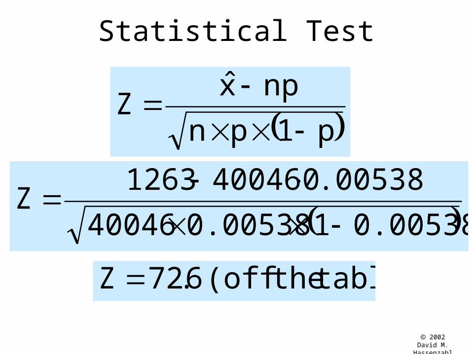
Statistical Test
0.0053810.0053840046
.00538040046 1263Z
p1pn
np x̂Z
table) the(off 6.72Z
2002
David M. Hassenzahl
Risk of Cholera?
• RR Lambeth versus rest of London is less than one
• IF Snow found a suitably unbiased, accurate, precise, etc estimator
• THEN Cholera is probably water-borne!

2002
David M. Hassenzahl
Benzene and Cancer
• Given Pliofilm data
• Is benzene a human carcinogen?
• Is benzene a human carcinogen at low concentrations?
• How potent is it?– RR is basically a linear estimator

2002
David M. Hassenzahl
Pliofilm Data (SWRI Page 215)
Cum. Expose
ppm-years
Leuke-mia
Range Mean Person years
Observe deaths
Expected per yr
0-45 11 30482 6 6.16
45-400 151 16320 6 3.84
400-1000 602 4667 3 1.58
>1000 1341 915 6 0.440
Total 132 52584 21 12.1

2002
David M. Hassenzahl
Pliofilm
• Rubber manufacturer
• Retrospective cohort study
• Recreated exposure
• Many effects
• Think about potential uncertainties!
2002
David M. Hassenzahl
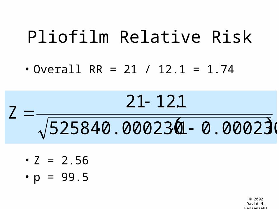
Pliofilm Relative Risk
• Overall RR = 21 / 12.1 = 1.74
• Z = 2.56
• p = 99.5
0.00023010.00023052584
1.12 21Z

2002
David M. Hassenzahl
Meaning of RR?
• Is there a threshold?– RR a bit less than one for lowest group– Calculate Z-score (not significant)
• What is RR excluding lowest group?
• Is there a non-linear effect?

2002
David M. Hassenzahl
P(leukemia|exposure)
0
0.1
0.2
0.3
0.4
0.5
0.6
0.7
0 500 1000 1500 2000
Mean exposure (ppm-years)
P *
100

2002
David M. Hassenzahl
P(leukemia|exposure)
0
0.1
0.2
0.3
0.4
0.5
0.6
0.7
0 500 1000 1500 2000
Low exposure (ppm-years)
P *
100

2002
David M. Hassenzahl
P(leukemia|exposure)
0
0.1
0.2
0.3
0.4
0.5
0.6
0.7
0 500 1000 1500 2000
High exposure (ppm-years)
P *
100

2002
David M. Hassenzahl
P(leukemia|cumulative exposure)
0
0.1
0.2
0.3
0.4
0.5
0.6
0.7
0 500 1000 1500 2000
Cumulative exposure (ppm-years)
P *
100

2002
David M. Hassenzahl
What about benzene?
• Probably a cause of leukemia and other cancers in humans
• Data suggest a threshold– But maybe not– Or is benzene hormetic?
• Lots of uncertainty

2002
David M. Hassenzahl
Conclusions
• Epidemiology and Toxicology are useful tools
• We HAVE to make assumptions
• We don’t know what “X” does– X = benzene, ionizing radiation, Alar…
• We have to decide what to do about X– Even if that means do nothing

2002
David M. Hassenzahl
Lessons Learned
• Managing types and sources of uncertainty
• Adding toolbox items– Bootstrapping, likelihood maximization,
spreadsheet skills, extrapolation
• If you are better informed but less certain now than several weeks ago, I’ve done my job

2002
David M. Hassenzahl
References
Aldrich, T and Griffith, J., Eds. (1993). Environmental Epidemiology and Risk Assessment, Van Nostrand Reinholt, NY NY.
Cox, L.A. (1995). “Reassessing benzene risks using internal doses and Monte-Carlo Uncertainty analysis.” Environmental Health Perspectives 104(Suppl.6):1413-29.
Gots, Ronald (1993). Toxic risks : science, regulation, and perception, Boca Raton, Lewis Publishers.
Kammen, D.M. and Hassenzahl, D.M. (1999). Should We Risk It? Exploring Environmental, Health and Technological Problem Solving Princeton University Press, Princeton NJ
Krump, K.S. and Allen, B.C. (1984). Quantitative Estimates of the Risk of Leukemia from Occupational Exposures to Benzene. Final Report to the OSHA. Ruston, LA: Science Research Systems
US EPA (1997) “Proposed Guidelines for Carcinogen Risk Assessment.” Federal Register 61(79) (April 23) 17960-18011.

2002
David M. Hassenzahl

2002
David M. Hassenzahl

2002
David M. Hassenzahl